Abstract
Dwell time is a critical factor in constructing and adjusting railway timetables for efficient and accurate operation of railways. This paper develops dwell time estimation models for a Shinbundang line (S line) in Seoul, South Korea using support vector regression (SVR), multiple linear regression (MLR), and random forest (RF) techniques utilizing archived real-time metro operation data along with smart card-based passenger information. In the first phase of this research, the collected data are processed to extract boarding and alighting passenger counts and observed dwell times of each train at all stations of the S line under the current operational environment. In the second phase, we develop SVR, MLR, and RF-based dwell time estimation models. It is found that the SVR-based model successfully estimates the dwell times within 10 s of differences for 84.4% of observed data. The results of this paper are especially beneficial for autonomous railway operations that need constructing and maintaining dynamic railway timetables that require reliable dwell time predictions in real-time.
1. Introduction
The relatively reliable schedule adherence of railway systems is one of the most attractive merits of the mode for the railway passengers [1]. However, it is still a challenge to operate on railways with perceived reliability. Railway schedules are constructed based on passenger demand, although the arrival patterns of passengers at stations are not uniform or deterministic in real-life. If a particular train’s arrival at a station is delayed, an additional accumulation of arriving passengers in the meantime will result in extended boarding and alighting times when the train dwells at the station, and this event will further propagate delays with respect to subsequent trains upstream.
Railway operators and authorities have considered different strategies when determining train schedules with respect to stations with expected passenger demands. They employ a “running time supplement” [2,3], a buffering time that can help to recover from delays if they occur. To minimize the delay, larger railway operators often control the passenger demand with a more direct approach of employing dedicated personnel on the platforms at stations, who can restrict passengers from boarding trains when they are delayed. There have been various studies in predicting delays and analyzing their intrinsic nature [2,3], timetable optimization [4,5,6,7], developing appropriate performance indices, and utilizing them for timetable construction [8].
For railway-related research, it is essential to have access to real-life data, including the operation of trains and passenger flows, while a larger amount of data will further benefit the reliability of the analysis. Automatic passenger counters (APCs) and smart card-based fare payment systems have been utilized for such purposes. Um et al. [9] utilized big data based on the smart card system in Seoul, South Korea for assessing performance measures of the public transit services including schedule adherence and crowdedness of passengers. Using smart card-based passenger fare and rail operation data, Hong et al. [10] developed models for predicting actually taken passenger-routes, the number of boarding and alighting passengers at stations, and the number of passengers on board between stations. Berbey et al. [11] used data from Line 1 of the Panama Metro and passengers’ preferences of train ticket classes in order to estimate dwell times at each station. Lam et al. [12] developed a regression model to investigate the relationship between dwell time and the number of boarding and alighting passengers, and tested it using Monte-Carlo simulations. Lee et al. [13] developed a timetable adjustment model for the Hong Kong metro, MTR, by analyzing the departure and arrival information of trains, boarding and alighting passenger counts at stations, and historical data of past causes of delays. Markovic et al. [14] developed a machine learning model based on a support vector regression method for predicting delays at railway stations operated with different classes of trains. Wang and Work [15] proposed a regression-based estimation model for future train delays using only the operation records of trains. Despite numerous efforts in research works regarding train delays, there have not been any significant research works for modeling dwell/delay time of trains utilizing boarding and alighting passenger counts, or onboard crowdedness (load factor), for all trains at all train stations of a metro line. Jiang et al. [16] conducted a similar line of research for Line 8 of the Shanghai Metro in China, yet with limited data and simulated values for load factor, boarding, and alighting passenger counts. Adachi et al. [17] adopted a Gompertz curve to overcome a limited data set of boarding and alighting passenger counts collected at 30-min intervals.
A smart card-based transit fare system has been in use in Seoul, South Korea since 2004 and currently 99% of all passengers use the smart card, which provides an excellent basis to collect real-life data for passenger flows. The smart card-based database includes each passenger’s origin and destination stops or stations, associated times, transit transfer locations, etc. This paper utilizes data from real-life operations of trains in the Seoul Metro, and the smart card-based passenger information, for estimating dwell times for each station of a metro line. Section 2 describes the data structures of train operations and smart card-based passengers’ information, and how the two databases are processed for further analysis. Section 3 develops a methodology based on extracting observed dwell times for each station using real-time data of train operations. Section 4 uses the observed dwell times, along with boarding and alighting passenger counts, onboard loading factors, to estimate dwell times. Section 5 concludes the paper.
2. Matching the Automatic Fare Collection Data with the Real-Time Train Operation Data
This paper develops a dwell time estimation model using boarding and alighting passenger counts, and onboard passenger counts between stations for each train. The initial dataset for analysis was prepared according to the method suggested by Hong et al. [10] based on the smart card passenger information and archived real-time train operation data. This dataset includes the number of trains operating and their current status with respect to their nearest station as one of 3 stages—“approaching,” “arrival,” and “departure”—along with timestamps for when the current stage was acquired. The approaching status is gained as soon as the arriving train passes a balise located at 1000 m upstream of an associated station. The arrival status is achieved as soon as the train passes a balise located 400 m upstream. The status changes to departure when the train passes a balise at 200 m downstream. The smart card-based passenger information includes the serial number of the card, boarding station, boarding time, alighting station, alighting time, transfer station, and transfer time. It is noted that the time associated with boarding, alighting, and transfer refers to the time when the passenger checks in or out with the gates at stations.
In this paper, both archived real-time train operation and smart card-based passenger data from the Shinbundang line (S Line) on 31st October 2017 was used. The S line has concentrated commuting passenger demands during both morning and afternoon peak periods, with dominating directions of the majority of passengers: towards the CBD in the morning and towards Bundang in the afternoon (See Figure 1). In this study, to show the morning peak clearly with maximum crowdedness, the S line’s Central Business District (CBD)-bound direction towards Gangnam station was selected for the analysis. The S line has a total length of 31.29 km, consisting of 12 stations, of which 4 stations allow inter-line transfers. The fleet size is 20 trains, and they run 327 cycles and 271 cycles in total on weekdays and weekend days, respectively; mostly throughout the entire route, except for the first and last trains each day. There is only 1 class of tickets, and daily ridership on the S line is roughly 247,000, as of 2017. For train operation data, arrival and departure times were identified for each train and each station. However, in cases where departure data were missing, average dwell times based on visual observations with video cameras were added to the arrival times to estimate the missing departure times.
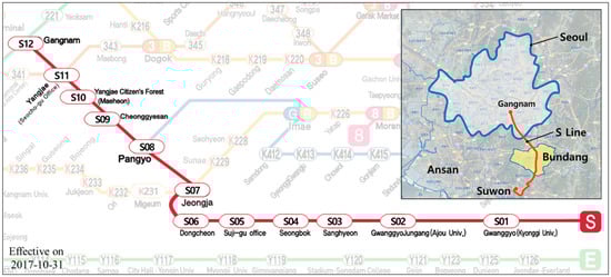
Figure 1.
Route map and the station ID of Shinbundang S line.
Figure 2 shows the process of matching the smart card passenger information with the archived real-time train operation data. The process starts with identifying a passenger who has alighted at a station. Then, the train that arrived at the station most recently is assumed to be the one that the passenger got off from. The departure time of the train that the passenger had boarded earlier is found. If the boarding time is earlier than the departure time of the train, the train number is assigned to that passenger, assuming that the passenger has boarded and will alight from that train. If the matching process does not succeed, the data from the smart card is not used, since there may be logical errors in the data. This is reasonable, because there is no way to reduce the travel time by overtaking between trains, or transferring through the other lines since the S line has a single class of train. The process stops when the number of the smart-card data that have been processed is equal to the total number of the smart-card data, N.
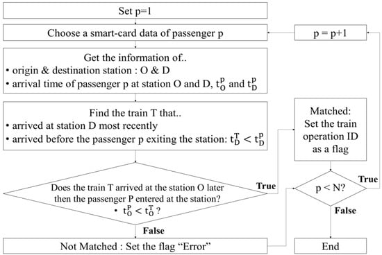
Figure 2.
Smart card-based passenger information matching process against the real-time train operation data.
Figure 3 shows smart card-based passenger data and train operation data from the S07 station to the S11 station in a passenger entry-exit map suggested by Hong et al. [10]. The x-axis represents the time at the S07 station, and the y-axis represents the time at the S11 station. Circles, triangles, and plus signs represent groups of individual passenger’s smart card data who have completed their trips from S07 to S11 with associated boarding and alighting times at those stations. Train number 477 arrives at the S07 at 7:25:56 and S11 at 7:38:02. Any potential passengers who were on train 477 during the trip must be on the 2nd quadrant of the horizontal and vertical lines intersecting at train 477. If the passengers used train 477, they must pass the boarding gate at S07 station before train 477 arrives at S07 station, and must also alight after the train arrives at S11 station. Therefore, the group of passengers surrounded by the dotted lines roughly represents all of the potential users of train 477 from S07 to S11 station. It is noted that there were some passengers who boarded and alighted at the same stations, and these were excluded from the analysis.
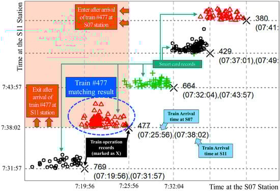
Figure 3.
Entry-exit map of the trip from Jeongja (S07) station to Yangjae (S11) station.
Figure 4 shows the number of passengers boarding, alighting, and arriving onboard at each station on the S line. Trains depart from the right towards the left, and each line in each graph represents a train. Red lines represent trains operated during the morning peak-hours from 6:30 a.m. to 10:30 a.m., and blue lines represent trains run during the afternoon-peak hours from 6:00 p.m. to 9:00 p.m. Trains run outside of peak-hours are represented by gray lines.
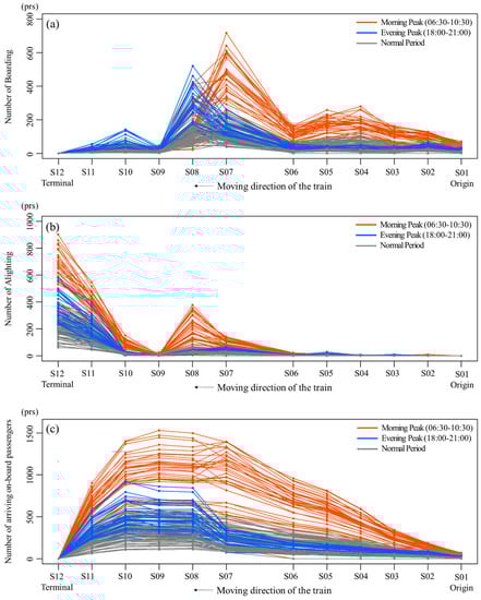
Figure 4.
(a) The number of boarding passengers at each station. (b) The number of alighting passengers at each station. (c) The number of onboard passengers when the train had been arrived at each station.
Figure 4 shows passenger boarding, alighting and onboard counts. When observed from the right, starting with the first station S01, in the morning peak, the boarding counts from S01 to S08 stations, inclusive, are significantly higher than the rest of stations combined. This is due to the fact that the regions covered by stations from S01 to S08 are dedicated residential areas (bed towns) of the Greater Seoul Area (GSA), S09 and S10 are located in an outskirts of Seoul, and S11 and S12 are located in the CBD of Gangnam area of Seoul. During the evening peak period, boarding counts at the S08 station stands out as there is also a large concentrated commercial area called “Pangyo Techno Valley”. This area is also related to the high number of alighting at S08 in the morning.
During the morning peak-hour period, at stations from S01 to S06, inclusive, and S09, there are nearly zero alighting passengers. At S07 and S08 stations, some passengers alight, while most of the passengers alight at S11 and S12 stations in the CBD. There are relatively high numbers of alighting passengers at S07 and S08 compared to other residential areas because there are concentrations of office buildings near those stations. Note that S07 and S08 also serve as transfer stations connected with other metro lines. In the case of station S09, there are only residential facilities near the station, hence resulting in very low alighting counts. In the afternoon-peak and non-peak periods, most alighting counts occur at S11 and S12 stations.
Due to the various characteristics mentioned earlier, the onboard passenger counts, as shown in Figure 4c, continue to increase as trains approach the final station S12 in the CBD. It is also noted that most trains in the morning-peak period experience passengers occupying at the full capacity of the trains and even exceeding the capacity with a factor of 2 between the S07 and S11 stations.
3. Estimating Observed Dwell Time of Train When Departure Information Is Missing
This paper utilizes the real-time operation data of the metro trains. The collected data have relatively well-recorded arrival times of trains, while often missing the departure times. Therefore, in cases where the departure times are missing, the observed dwell time for each train at each station was estimated by using typical travel times between stations.
As illustrated in Figure 5, the train arrival times at station S and S + 1 is easily determined from the train operation data. The arrival time refers to the time when a train passes 400 m upstream of an associated station. The time difference between the 2 stations consists of the braking time at station S (BS), dwell time at station S (DWS), and the travel time between the station S and 400 m upstream location of station S + 1. If we assume the braking times are similar for all stations, the braking time at station S (BS) can be subtracted from the time difference between the two stations S and S + 1 in order to estimate the actual dwell time. The S line, from which the data were collected, is specifically suitable for such assumptions, because it is autonomously operated and has constant braking times at stations with a large headway of 4 min, and has a relatively low chance of congestion occurring due to the influence of trains downstream. The assumption of constant braking times was verified visually with video cameras installed on all trains. Figure 6 shows the time difference between arrivals of trains at all stations (solid black and red lines), and average travel times visually observed from trains equipped with video cameras (blue dotted line). The difference, DWS, between the TTS and TDS is the estimated dwell time for each train at each station in the case of missing departure data. It is noted that the red lines represent time difference between arrivals at stations of the first 5 trains in the early morning period, where there are no delays, while black lines represent for all other trains.
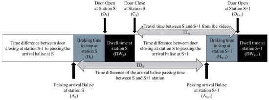
Figure 5.
Time components of railway operation between stations and definitions of TTS and TDS.
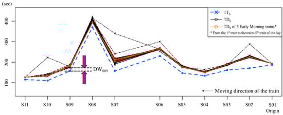
Figure 6.
TTS and TDS at each station and the concept of estimating the DWS at each station.
Figure 7 shows a relationship between the estimation of observed dwell times for all trains at all stations versus the sum of boarding and alighting passenger counts. The x-axis represents the sum of boarding and alighting passengers while the y-axis represents the estimation of observed dwell times. Each symbol represents a station, as illustrated in Table 1. The minimum observed dwell time is 16 s. The variability of dwell times is found to be larger when the passenger counts are smaller, and smaller when the passenger counts are larger. In addition, it is found that the minimum dwell time increases as the passenger counts increase. It is interesting to note that many observed dwell times at certain stations seem to have constant dwell times regardless of passenger counts. This is a result of enforced dwell times at some major stations being assisted by dedicated employees on the platforms, limiting the number of boarding passengers.
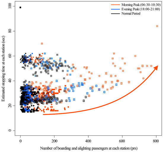
Figure 7.
Relationship between estimated dwell time and the number of boarding and alighting passengers at each station of S line.

Table 1.
Symbols of each station.
4. Dwell Time Estimation Model
In this second phase of research, we utilize the results from the first phase, including the observed dwell times (which required estimations when the departure information was missing), boarding and alighting passenger counts for all trains at all stations, in order to develop dwell time estimation models. The proposed models estimate dwell times at all stations with given boarding and alighting passenger counts and onboard passenger counts on arriving trains.
Boarding, alighting, and onboard passenger counts for each train at each station are set as independent variables and the dwell time as dependent variable. This is intuitive, as dwell times are mainly affected by the boarding and alighting counts, while the onboard crowdedness in trains indirectly affects them. The dependent variable, dwell time, was extracted from the observed data as described in Section 3. Support Vector Regression (SVR), Multiple Linear Regression (MLR), and Random Forest (RF) methods were used to develop 3 different estimation models, and their estimation performances were compared. Seventy percent of the data were used as a training set to develop the model, and 30% of the data were used as a validation set.
To compare the performances of the different models, performances were compared for 3 different scenarios of dwell time estimation accuracy of less than 3, 5, and 10 s between the actual and estimated dwell times. Among the validation set, the SVR model shows that 53.6% of cases have less than 3 s of errors, and 67.2% have less than 5 s of errors. On the other hand, 87.5% of the estimation by the RF model in the validation set marked below 10 s of error, as shown in Table 2. It is noted that the dwell times used for training are in integer values while the estimated dwell times from the models are in real numbers, and making distinctions between the 3 scenarios separated by a few seconds may be practically insignificant in real-life metro operations.
Table 2.
The proportion of estimated data depends on the absolute difference between actual dwell time and estimated dwell time by the model types.
When compared from the perspective of percentage accuracy, the SVR model performed the best in the case of less than 30% errors followed by RF and MLR models as seen in Table 3. Figure 8 and Figure 9 show the comparison of dwell time estimation results derived from each model. The orange square represents the trains operated during the morning peak hour, the blue circle represents the trains operated during the evening peak hour, and the black triangle represents the trains operated outside the two rush-hour periods.
Table 3.
The proportion of estimated data depends on the relative difference between actual dwell time and estimated dwell time by the model types.
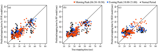
Figure 8.
Dwell time estimation performance comparison among the (a) SVR, (b) RF, (c) MLR models.
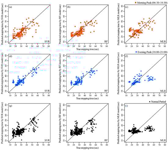
Figure 9.
Dwell time estimation performance comparison by the time of day. (a~c) in the morning peak, (d~f) in the evening peak and (g~i) in the normal period.
To further enhance the SVR model with 3 variables (with boarding, alighting, and onboard passenger counts at independent variables) which was found to be the most accurate model among the 3 models, we developed different SVR models with 3 additional input variables: train arrival time, station information, and time difference between arrivals at 2 consecutive stations. As shown in Table 4 and Table 5, it is found that the performances of SVRs with additional input variables were further enhanced. In particular, the scenario with less than 5 s of error was improved by 20% in accuracy. Most notably, the enhanced SVR model performed at 97.2% accuracy for the scenario with less than 10 s of error. Figure 10 shows the comparison of estimation performance between the 6-variable model with the 3-variable model.
Table 4.
The proportion of estimated data depends on the absolute difference between actual dwell time and estimated dwell time by the number of variables of SVR models.
Table 5.
The proportion of estimated data depends on the relative difference between actual dwell time and estimated dwell time by the number of variables of SVR models.
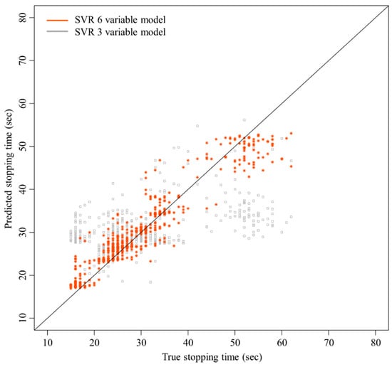
Figure 10.
Estimation performance of the 6-variable and the 3-variable SVR model.
5. Conclusions
This paper develops a railway dwell time estimation model using SVR, RF, and MLR methods. In the first phase, smart card-based passenger information is matched against the real-time train operation data from the S line of the Seoul Metro in Seoul, South Korea, for extracting boarding, alighting, on-bard passenger counts, and the observed dwell times for all trains at all stations. When the train departure times were missing, an assumption of constant braking time was adopted to estimate actual/observed dwell times, since the S line is autonomously operated with minimal variability in braking times.
In the second phase, the paper develops dwell time estimation models utilizing the extracted information from the first phase. The SVR, RF and MLR-based models were developed for dwell time estimations while boarding, alighting, and onboard passenger counts were treated as independent variables and the dwell time was set as a dependent variable. In the comparative scenarios with less than 3, 5, and 10 s of errors between the estimations and the observed values, the SVR model performed the best, with an accuracy of 67.2% in the scenario with less than 5 s of error. Then the SVR model was enhanced by including additional independent variables, including arrival times and time difference of arrivals, at 2 consecutive stations for all trains at all stations. It was found that the enhanced SVR model improved the accuracy by 20% to an accuracy of 87.6% for the scenario of less than 5 s of error. In the case of less than 10 s of error, the improved SVR model performed at 97.2% accuracy.
This research is unique in the sense that, firstly, it extracts boarding, alighting, and onboard passenger counts using data from real-life metro operations and smart card-based passenger information for all trains at all stations on an urban metro line. Secondly, this research develops dwell time estimation models with high performance accuracies that are validated by real-life data. The results of this paper are especially beneficial for autonomous railway operation, which requires construction and maintenance of dynamic railway timetables that require reliable dwell time real-time predictions. However, this estimation model may not work well if incidents such as rolling stock failure, or big events (i.e., sports games or exhibitions) occur near metro stations that may increase the demand dramatically and present unseen data to the proposed models. Enhancing the proposed estimation models to cover not only a general commute-based operation environment, but also the situations affected by such special events, are topics of future studies.
Author Contributions
In this study, all of the authors contributed to the writing of the manuscript. Y.O. designed the overall modeling framework and performed the data analysis. Y.-J.B. helped with the data analysis and drafted the initial version of the manuscript. J.Y.S. supported data acquisition and contributed to the results interpretation. H.-C.K. and S.K. advised on the modeling process and coordinated the overall research. All authors have read and agreed to the published version of the manuscript.
Funding
This research was supported by a grant from R&D Program of the Korea Railroad Research Institute, Republic of Korea.
Acknowledgments
The authors thank Seong-Jong Woo and Soo-In Lee for their help in data processing.
Conflicts of Interest
The authors declare no conflict of interest.
References
- Parbo, J.; Nielsen, O.A.; Prato, C.G. Passenger Perspectives in Railway Timetabling: A Literature Review. Transp. Rev. 2016, 36, 500–526. [Google Scholar] [CrossRef]
- Goverde, R.M.P. A delay propagation algorithm for large-scale railway traffic networks. Transp. Res. Part C Emerg. Technol. 2010, 18, 269–287. [Google Scholar] [CrossRef]
- Harrod, S.; Cerreto, F.; Nielsen, O.A. A closed form railway line delay propagation model. Transp. Res. Part C Emerg. Technol. 2019, 102, 189–209. [Google Scholar] [CrossRef]
- Liebchen, C. The first optimized railway timetable in practice. Transp. Sci. 2008, 42, 420–435. [Google Scholar] [CrossRef]
- Harrod, S.S. A tutorial on fundamental model structures for railway timetable optimization. Surv. Oper. Res. Manag. Sci. 2012, 17, 85–96. [Google Scholar] [CrossRef]
- Cucala, A.P.; Fernández, A.; Sicre, C.; Domínguez, M. Fuzzy optimal schedule of high speed train operation to minimize energy consumption with uncertain delays and driver’s behavioral response. Eng. Appl. Artif. Intell. 2012, 25, 1548–1557. [Google Scholar] [CrossRef]
- Högdahl, J.; Bohlin, M.; Fröidh, O. A combined simulation-optimization approach for minimizing travel time and delays in railway timetables. Transp. Res. Part B Methodol. 2019, 126, 192–212. [Google Scholar] [CrossRef]
- Goverde, R.M.P.; Hansen, I.A. Performance indicators for railway timetables. In Proceedings of the IEEE International Conference on Intelligent Rail Transportation, Beijing, China, 30 August–1 September 2013; pp. 301–306. [Google Scholar]
- Eom, J.K.; Song, J.Y.; Moon, D.S. Analysis of public transit service performance using transit smart card data in Seoul. KSCE J. Civ. Eng. 2015, 19, 1530–1537. [Google Scholar] [CrossRef]
- Hong, S.P.; Min, Y.H.; Park, M.J.; Kim, K.M.; Oh, S.M. Precise estimation of connections of metro passengers from Smart Card data. Transportation 2016, 43, 749–769. [Google Scholar] [CrossRef]
- Alvarez, A.B.; Merchan, F.; Poyo, F.J.C.; George, R.J.C. A fuzzy logic-based approach for estimation of dwelling times of panama metro stations. Entropy 2015, 17, 2688–2705. [Google Scholar] [CrossRef]
- Lam, W.H.K.; Cheung, C.Y.; Poon, Y.F. A Study of Train Dwelling Time at the Hong Kong Mass Transit Railway System. J. Adv. Transp. 1998, 32, 285–296. [Google Scholar] [CrossRef]
- Lee, W.H.; Yen, L.H.; Chou, C.M. A delay root cause discovery and timetable adjustment model for enhancing the punctuality of railway services. Transp. Res. Part C Emerg. Technol. 2016, 73, 49–64. [Google Scholar] [CrossRef]
- Marković, N.; Milinković, S.; Tikhonov, K.S.; Schonfeld, P. Analyzing passenger train arrival delays with support vector regression. Transp. Res. Part C Emerg. Technol. 2015, 56, 251–262. [Google Scholar] [CrossRef]
- Wang, R.; Work, D.B. Data Driven Approaches for Passenger Train Delay Estimation. In Proceedings of the 18th International Conference on Intelligent Transportation Systems, Las Palmas, Spain, 15–18 September 2015; pp. 535–540. [Google Scholar]
- Jiang, Z.; Xie, C.; Ji, T.; Zou, X. Dwell time modelling and optimized simulations for crowded rail transit lines based on train capacity. Promet Traffic Transp. 2015, 27, 125–135. [Google Scholar] [CrossRef][Green Version]
- Adachi, S.; Yoshino, H.; Koresawa, M.; Parady, G.T.; Takami, K.; Harata, N. A Study on Train Travel Time Simulation Focused on Detailed Dwell Time Structure and on-site Inspections. In Proceedings of the 8th International Conference on Railway Operations Modelling and Analysis (ICROMA), Norrköping, Sweden, 17–20 June 2019; pp. 15–28. [Google Scholar]


© 2020 by the authors. Licensee MDPI, Basel, Switzerland. This article is an open access article distributed under the terms and conditions of the Creative Commons Attribution (CC BY) license (http://creativecommons.org/licenses/by/4.0/).