Portfolio Optimization-Based Stock Prediction Using Long-Short Term Memory Network in Quantitative Trading


Abstract
1. Introduction
- The LSTM prediction model was proposed to predict stock price in order to construct and optimize portfolios in quantitative trading.
- Presenting a comparison between LSTM prediction model performance to gated recurrent units (GRUs) and other conventional machine learning models such as linear regression (LR) and support vector regression (SVR) for stock prediction.
- Simulation modeling and optimization modeling approaches were used to optimize portfolios in quantitative trading.
- Finally, portfolio performance evaluation for the constructed portfolios was conducted in which our constructed portfolios outperform the benchmark on both active return and risk control.
2. Background and Literature Review
2.1. Fundamentals of Quantitative Trading
2.2. Quantitative Portfolio Management
2.2.1. Portfolio Construction
2.2.2. Portfolio Optimization
2.2.3. Portfolio Performance Evaluation
2.3. Deep Learning in Stock Prediction
3. Methodology
3.1. Prediction Model
3.2. Quantitative Models
3.2.1. Multiple Assets Portfolio Construction
3.2.2. Portfolio Optimization
- Simulation Modeling: Monte Carlo Simulation (MCS)
| Algorithm 1: Pseudocode of the Monte Carlo Simulation |
Input
|
Output
|
| foriinrange(n): |
|
- 2.
- Optimization Modeling: Mean-variance Optimization (MVO)
| Minimize (w) | |
| s.t | |
4. Experiment and Results
4.1. Data Collection and Experiment Design
4.2. Performance Evaluation
4.2.1. Stock Prediction Evaluation
4.2.2. Portfolio Performance Evaluation
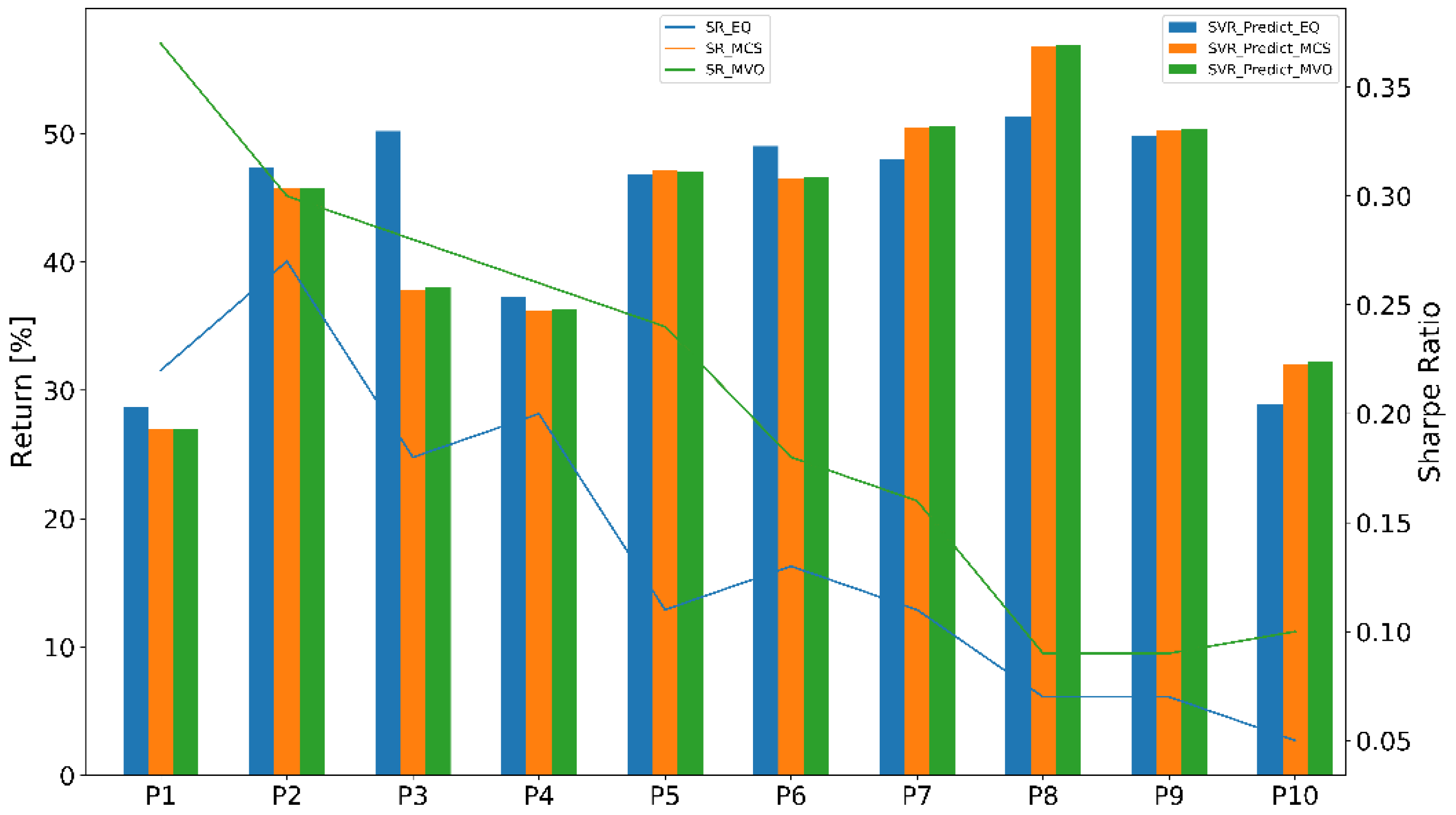
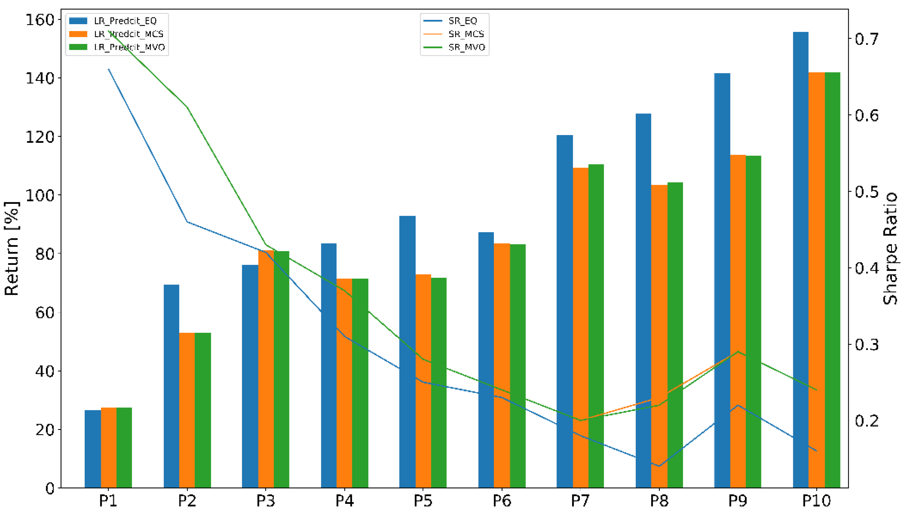
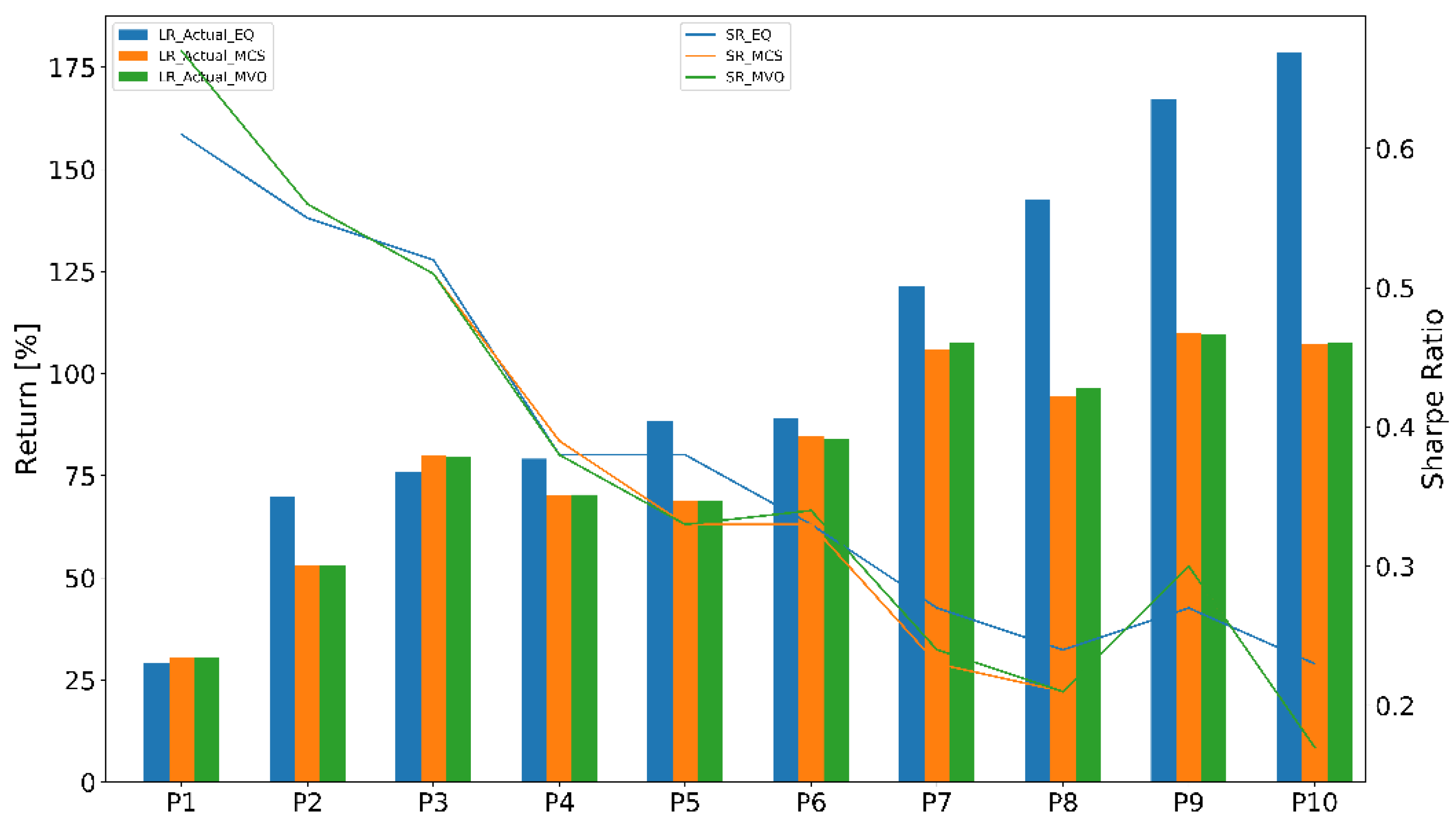
- Equal-weighted portfolio (EQ) is a type of weighting that gives the same weight to each stock in a portfolio. In our work, we chose initial weight .
- Monte Carlo simulation (MCS) was used to find the optimal weights of thousands of scenarios or iterations. The number of iterations is n = 50,000.
- Mean-variance optimization (MVO) was used to find an adaptive weights portfolio that adapted the stock weights using the prediction models.
4.3. Experiment Results
4.3.1. Stock Prediction Results
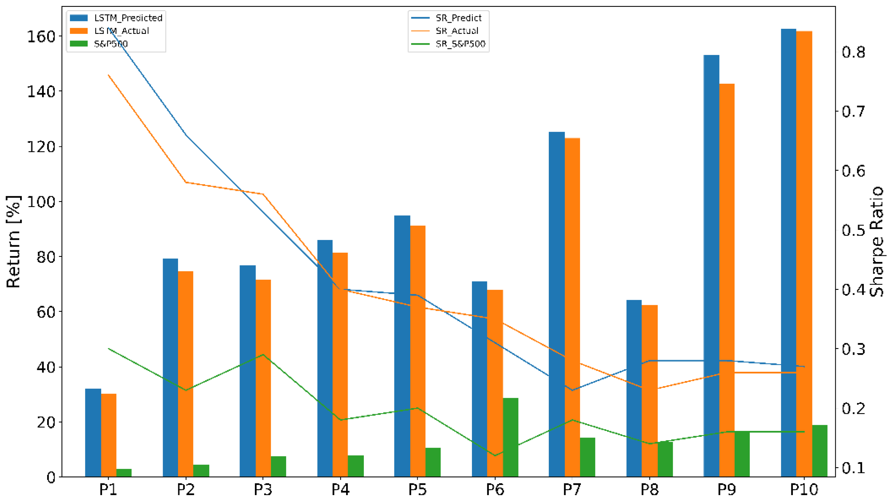
4.3.2. Portfolio Performance Evaluation
5. Conclusions and Discussions
Author Contributions
Funding
Conflicts of Interest
References
- Fabozzi, F.J.; Markowitz, H.M. The Theory and Practice of Investment Management: Asset Allocation, Valuation, Portfolio Construction, and Strategies, 2nd ed.; John Wiley and Sons: Hoboken, NJ, USA, 2011; Volume 198, pp. 289–290. [Google Scholar]
- Adebiyi, A.A.; Adewumi, A.O.; Ayo, C.K. Comparison of ARIMA and artificial neural networks models for stock price prediction. J. Appl. Math. 2014. [Google Scholar] [CrossRef]
- Cumming, J.; Alrajeh, D.D.; Dickens, L. An Investigation into the Use of Reinforcement Learning Techniques Within the Algorithmic Trading Domain. Master’s Thesis, Imperial College London, London, UK, 2015. [Google Scholar]
- Chong, E.; Han, C.; Park, F.C. Deep learning networks for stock market analysis and prediction: Methodology, data representations, and case studies. Expert Syst. Appl. 2017, 83, 187–205. [Google Scholar] [CrossRef]
- Fabozzi, F.J.; Pachamanova, D.A. Portfolio Construction, and Analytics; John Wiley & Sons: Hoboken, NJ, USA, 2016; pp. 111–112. [Google Scholar]
- Kissell, R.L. The Science of Algorithmic Trading and Portfolio Management; Academic Press: Cambridge, MA, USA, 2013; pp. 111–112. [Google Scholar]
- Ta, V.D.; Liu, C.M.; Addis, D. Prediction and Portfolio Optimization in Quantitative Trading Using Machine Learning Techniques. In Proceedings of the Ninth International Symposium on Information and Communication Technology, Da Nang, Vietnam, 6–7 December 2018; pp. 98–105. [Google Scholar]
- Six Asset Allocation Strategies that Work. Available online: https://www.investopedia.com/investing/6-asset-allocation-strategies-work/ (accessed on 4 October 2019).
- Markowitz, H. Portfolio selection. J. Financ. 1952, 7, 779–781. [Google Scholar]
- Sharpe, W.F.; Sharpe, W.F. Portfolio Theory and Capital Markets; McGraw-Hill: New York, NY, USA, 1970; Volume 217. [Google Scholar]
- Roll, R.; Ross, S.A. An empirical investigation of the arbitrage pricing theory. J. Financ. 1980, 35, 1073–1103. [Google Scholar] [CrossRef]
- Fama, E.F.; French, K.R. Common risk factors in the returns on stocks and bonds. J. Financ. Econ. 1993, 33, 35–36. [Google Scholar] [CrossRef]
- He, G.; Litterman, R. The Intuition Behind Black-Litterman Model Portfolios; Goldman Sachs Investment Management Research: New York, NY, USA, 1999. [Google Scholar]
- Kolm, P.N.; Tutuncu, R.; Fabozzi, F.J. 60 Years of portfolio optimization: Practical challenges and current trends. Eur. J. Oper. Res. 2014, 234, 356–371. [Google Scholar] [CrossRef]
- Ahmadi-Javid, A.; Fallah-Tafti, M. Portfolio optimization with entropic value-at-risk. Eur. J. Oper. Res. 2019, 279, 225–241. [Google Scholar] [CrossRef]
- Lejeune, M.A.; Shen, S. Multi-objective probabilistically constrained programs with variable risk: Models for multi-portfolio financial optimization. Eur. J. Oper. Res. 2016, 252, 522–539. [Google Scholar] [CrossRef]
- Lwin, K.T.; Qu, R.; Mac Carthy, B.L. Mean-VaR portfolio optimization: A nonparametric approach. Eur. J. Oper. Res. 2017, 260, 751–766. [Google Scholar] [CrossRef]
- Qin, Z. Mean-variance model for portfolio optimization problem in the simultaneous presence of random and uncertain returns. Eur. J. Oper. Res. 2015, 245, 480–488. [Google Scholar] [CrossRef]
- Samarakoon, L.P.; Hasan, T. Portfolio performance evaluation. Encyclopedia of Finance, 2nd ed.; Springer: New York, NY, USA, 2006; pp. 617–622. [Google Scholar]
- Aragon, G.O.; Ferson, W.E. Portfolio performance evaluation. Found. Trends Financ. 2007, 2, 831–890. [Google Scholar] [CrossRef]
- Elleuch, J.; Trabelsi, L. Fundamental analysis strategy and the prediction of stock returns. Int. Res. J. Financ. Econ. 2009, 30, 95–107. [Google Scholar]
- Sezer, O.B.; Ozbayoglu, A.M.; Dogdu, E. An artificial neural network-based stock trading system using technical analysis and big data framework. In Proceedings of the South East Conference, Haines, AK, USA, 4–12 April 2017; pp. 223–226. [Google Scholar]
- Fang, L.; Yu, H.; Huang, Y. The role of investor sentiment in the long-term correlation between US stock and bond markets. Int. Rev. Econ. Financ. 2018, 58, 127–139. [Google Scholar] [CrossRef]
- Nguyen, T.H.; Shirai, K.; Velcin, J. Sentiment analysis on social media for stock movement prediction. Expert Syst. Appl. 2015, 42, 9603–9611. [Google Scholar] [CrossRef]
- Lam, M. Neural network techniques for financial performance prediction: Integrating fundamental and technical analysis. Decis. Support Syst. 2004, 37, 567–581. [Google Scholar] [CrossRef]
- Deng, S.; Mitsubuchi, T.; Shioda, K.; Shimada, T.; Sakurai, A. Combining technical analysis with sentiment analysis for stock price prediction. In Proceedings of the 2011 IEEE Ninth International Conference on Dependable, Autonomic and Secure Computing, Sydney, Australia, 12–14 December 2011; pp. 800–807. [Google Scholar]
- Sirignano, J.A. Deep learning for limit order books. Quant. Financ. 2019, 19, 549–570. [Google Scholar] [CrossRef]
- Sohangir, S.; Wang, D.; Pomeranets, A.; Khoshgoftaar, T.M. Big Data: Deep Learning for financial sentiment analysis. J. Big Data 2018, 5, 3. [Google Scholar] [CrossRef]
- Xiong, R.; Nichols, E.P.; Shen, Y. Deep Learning Stock Volatility with Google Domestic Trends. arXiv 2015, arXiv:1512.04916. [Google Scholar]
- Heaton, J.B.; Polson, N.G.; Witte, J.H. Deep learning for finance: Deep portfolios. Appl. Stoch. Models Bus. Ind. 2017, 33, 3–12. [Google Scholar] [CrossRef]
- Bao, W.; Yue, J.; Rao, Y. A deep learning framework for financial time series using stacked autoencoders and long-short term memory. PLoS ONE 2017, 12, e0180944. [Google Scholar] [CrossRef]
- Shen, F.; Chao, J.; Zhao, J. Forecasting exchange rate using deep belief networks and conjugate gradient method. Neurocomputing 2015, 167, 243–253. [Google Scholar] [CrossRef]
- Chung, J.; Gulcehre, C.; Cho, K.; Bengio, Y. Empirical Evaluation of Gated Recurrent Neural Networks on Sequence Modeling. arXiv 2014, arXiv:1412.3555. [Google Scholar]
- Fischer, T.; Krauss, C. Deep learning with long short-term memory networks for financial market predictions. Eur. J. Oper. Res. 2018, 270, 654–669. [Google Scholar] [CrossRef]
- Nguyen, T.T.; Yoon, S. A Novel Approach to Short-Term Stock Price Movement Prediction using Transfer Learning. Appl. Sci. 2019, 9, 4745. [Google Scholar] [CrossRef]


| Categories | Hyperparameters |
|---|---|
| Optimizer | Adam |
| The number of hidden layers | 2 |
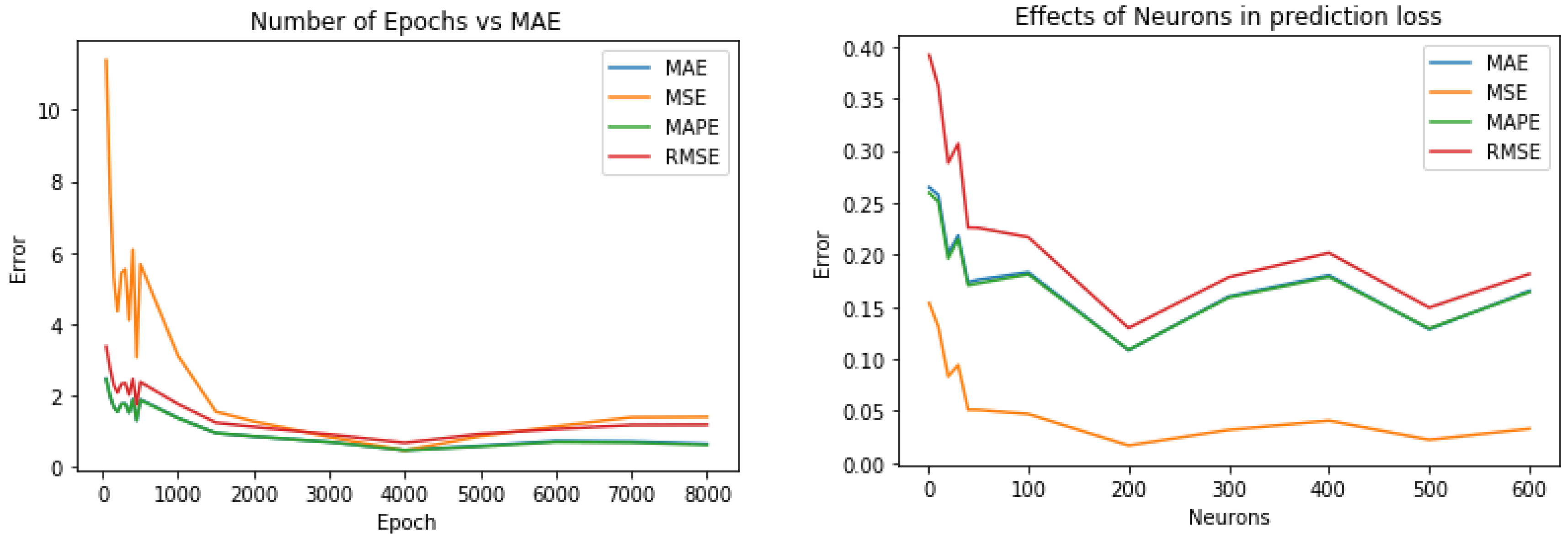
| The number of neurons | 512 and 256 |
| Number of epochs | 4000 |
| Period | Start | End | Days |
|---|---|---|---|
| 1 | 2017/11/22 | 2017/12/29 | 26 |
| 2 | 2017/10/17 | 2017/12/29 | 51 |
| 3 | 2017/09/12 | 2017/12/29 | 76 |
| 4 | 2017/08/07 | 2017/12/29 | 100 |
| 5 | 2017/06/30 | 2017/12/29 | 126 |
| 6 | 2017/05/25 | 2017/12/29 | 151 |
| 7 | 2017/04/19 | 2017/12/29 | 177 |
| 8 | 2017/03/14 | 2017/12/29 | 202 |
| 9 | 2017/02/06 | 2017/12/29 | 227 |
| 10 | 2016/12/29 | 2017/12/29 | 252 |
| P | LSTM | GRU | ||||
|---|---|---|---|---|---|---|
| Stock | MAE | MSE | Stock | MAE | MSE | |
| 1 | DVA | 0.05965 | 0.00413 | DVA | 0.04731 | 0.00258 |
| FCX | 0.01899 | 0.00064 | FCX | 0.02019 | 0.00067 | |
| KSS | 0.01364 | 0.00038 | M | 0.03484 | 0.00164 | |
| LB | 0.03459 | 0.00195 | LB | 0.02525 | 0.00092 | |
| 2 | FL | 0.04111 | 0.00279 | FL | 0.02515 | 0.00089 |
| NKTR | 0.01227 | 0.00024 | NKTR | 0.01232 | 0.00028 | |
| KSS | 0.01403 | 0.00035 | KR | 0.04080 | 0.00197 | |
| LB | 0.02482 | 0.00105 | LB | 0.02604 | 0.00105 | |
| 3 | MRO | 0.04735 | 0.00376 | MRO | 0.01433 | 0.00035 |
| NKTR | 0.04052 | 0.00236 | NKTR | 0.01565 | 0.00033 | |
| NATP | 0.02651 | 0.00124 | SIVB | 0.01357 | 0.00034 | |
| LB | 0.00850 | 0.00016 | LB | 0.04476 | 0.00302 | |
| 4 | GPS | 0.00321 | 0.00003 | GPS | 0.01324 | 0.00028 |
| NKTR | 0.00205 | 0.00001 | NKTR | 0.01554 | 0.00032 | |
| MU | 0.00230 | 0.00001 | MU | 0.01201 | 0.00025 | |
| URI | 0.00360 | 0.00002 | URI | 0.01473 | 0.01554 | |
| 5 | GPS | 0.01071 | 0.00019 | GPS | 0.01130 | 0.00021 |
| NKTR | 0.01347 | 0.00028 | NKTR | 0.01567 | 0.00035 | |
| NRG | 0.01485 | 0.00048 | NRG | 0.01461 | 0.00047 | |
| URI | 0.01726 | 0.00047 | URI | 0.01658 | 0.00046 | |
| 6 | ALGN | 0.01432 | 0.00043 | ALGN | 0.01034 | 0.00026 |
| NKTR | 0.00267 | 0.00002 | NKTR | 0.00114 | 0.00000 | |
| NRG | 0.01930 | 0.00044 | NRG | 0.00597 | 0.00005 | |
| TROW | 0.01360 | 0.00027 | URI | 0.01389 | 0.00029 | |
| 7 | ALGN | 0.00514 | 0.00004 | ALGN | 0.00892 | 0.00019 |
| NKTR | 0.00426 | 0.00004 | NKTR | 0.00367 | 0.00003 | |
| IPGP | 0.00294 | 0.00002 | NDVA | 0.01476 | 0.00037 | |
| NDVA | 0.00261 | 0.00002 | TTWO | 0.01806 | 0.00053 | |
| 8 | ABMD | 0.00813 | 0.00014 | ALGN | 0.01011 | 0.00021 |
| ADBE | 0.00756 | 0.00010 | IPGP | 0.00662 | 0.00008 | |
| ALGN | 0.00161 | 0.00000 | NKTR | 0.00186 | 0.00001 | |
| AMZN | 0.01258 | 0.00027 | NDVA | 0.01095 | 0.00021 | |
| 9 | ALGN | 0.00522 | 0.00006 | ABMD | 0.00847 | 0.00016 |
| IPGP | 0.01104 | 0.00030 | ADBE | 0.01157 | 0.00025 | |
| NKTR | 0.01319 | 0.00027 | ALGN | 0.00919 | 0.00012 | |
| TTWO | 0.02046 | 0.00063 | ATVI | 0.01863 | 0.00055 | |
| 10 | ALGN | 0.00751 | 0.00013 | ALGN | 0.00672 | 0.00010 |
| IPGP | 0.01134 | 0.00014 | IPGP | 0.00469 | 0.00005 | |
| NKTR | 0.00273 | 0.00002 | NKTR | 0.00505 | 0.00004 | |
| TTWO | 0.00969 | 0.00015 | TTWO | 0.01234 | 0.00027 | |
| P | Portfolio [%] | Benchmark [%] | Active Return [%] |
|---|---|---|---|
| 1 | 30.09 | 2.95 | 24.71 |
| 2 | 74.77 | 4.53 | 70.23 |
| 3 | 71.51 | 7.46 | 64.06 |
| 4 | 81.36 | 7.77 | 73.59 |
| 5 | 91.31 | 10.49 | 80.82 |
| 6 | 67.89 | 28.78 | 39.11 |
| 7 | 122.94 | 14.15 | 108.79 |
| 8 | 62.40 | 12.65 | 49.75 |
| 9 | 142.59 | 16.73 | 126.22 |
| 10 | 161.84 | 18.83 | 143.01 |
© 2020 by the authors. Licensee MDPI, Basel, Switzerland. This article is an open access article distributed under the terms and conditions of the Creative Commons Attribution (CC BY) license (http://creativecommons.org/licenses/by/4.0/).
Share and Cite
Ta, V.-D.; Liu, C.-M.; Tadesse, D.A. Portfolio Optimization-Based Stock Prediction Using Long-Short Term Memory Network in Quantitative Trading. Appl. Sci. 2020, 10, 437. https://doi.org/10.3390/app10020437
Ta V-D, Liu C-M, Tadesse DA. Portfolio Optimization-Based Stock Prediction Using Long-Short Term Memory Network in Quantitative Trading. Applied Sciences. 2020; 10(2):437. https://doi.org/10.3390/app10020437
Chicago/Turabian StyleTa, Van-Dai, CHUAN-MING Liu, and Direselign Addis Tadesse. 2020. "Portfolio Optimization-Based Stock Prediction Using Long-Short Term Memory Network in Quantitative Trading" Applied Sciences 10, no. 2: 437. https://doi.org/10.3390/app10020437
APA StyleTa, V.-D., Liu, C.-M., & Tadesse, D. A. (2020). Portfolio Optimization-Based Stock Prediction Using Long-Short Term Memory Network in Quantitative Trading. Applied Sciences, 10(2), 437. https://doi.org/10.3390/app10020437