Article

Towards Semi-Automatic Generation of a Steady State Digital Twin of a Brownfield Process Plant

1
Department of Electrical Engineering and Automation, Aalto University, 00076 Aalto, Finland
2
VTT Technical Research Centre of Finland Ltd., 02044 Espoo, Finland
3
Semantum Oy, 02150 Espoo, Finland
4
Department of Computer Science, Electrical and Space Engineering, Luleå University of Technology, 97187 Luleå, Sweden
*
Author to whom correspondence should be addressed.
Appl. Sci. 2020, 10(19), 6959; https://doi.org/10.3390/app10196959
Submission received: 26 August 2020 / Revised: 21 September 2020 / Accepted: 1 October 2020 / Published: 5 October 2020
(This article belongs to the Special Issue Digital Twins in Industry)

Abstract

:

Featured Application

A laboratory water heating and pressurizing process is used as a case study to demonstrate the proposed methodology for digital twin generation.

Abstract

Researchers have proposed various models for assessing design alternatives for process plant retrofits. Due to the considerable engineering effort involved, no such models exist for the great majority of brownfield process plants, which have been in operation for years or decades. This article proposes a semi-automatic methodology for generating a digital twin of a brownfield plant. The methodology consists of: (1) extracting information from piping and instrumentation diagrams, (2) converting the information to a graph format, (3) applying graph algorithms to preprocess the graph, (4) generating a simulation model from the graph, (5) performing manual expert editing of the generated model, (6) configuring the calculations done by simulation model elements and (7) parameterizing the simulation model according to recent process measurements in order to obtain a digital twin. Since previous work exists for steps (1–2), this article focuses on defining the methodology for (3–5) and demonstrating it on a laboratory process. A discussion is provided for (6–7). The result of the case study was that only few manual edits needed to be made to the automatically generated simulation model. The paper is concluded with an assessment of open issues and topics of further research for this 7-step methodology.

1. Introduction

Industrial process plants in sectors such as oil & gas, chemical, pulp & paper, power & heat, mineral processing, and water supply management have lifecycles of several decades. Retrofits offer a large potential for reductions in operating costs [1], energy consumption [2], CO2 emissions [3], freshwater consumption [4], and environmental pollution [5]. The said authors proposed various kinds of models for assessing these reductions at design phase. However, no such models exist for the great majority of brownfield process plants, due to the considerable engineering effort involved [6]. In this article a brownfield is defined as an operating plant, which has existing physical structures and legacy software systems. The plant design information at a brownfield plant is generally not in digital format [7].
A digital twin is a special kind of plant model that has been synchronized with the physical process using recent sensor information. Thus, a digital twin would be especially suited for designing retrofits for brownfield plants that have been in operation for a long time. The following requirements are identified for the digital twin:
  • It accurately captures aspects of the plant relevant to the retrofit
  • It can be generated from source information commonly available at brownfield plants
  • Minimal manual engineering effort should be involved
Despite much recent research on digital twins, there is a lack of research addressing these requirements. Numerous definitions for digital twins have been proposed. An experimentable digital twin, based on a simulation model of the plant, is suited for assessing impacts of a retrofit [8]. Simulation approaches for industrial process plants can be categorized into steady state and dynamic. Dynamic simulation has the special capability of determining how the process state changes over time in response to an event such as the closing of a valve or a setpoint change. Such capabilities are essential for investigating modernization of automation systems. A dynamic simulation model can be extended to an experimentable digital twin through tracking approaches that synchronize the simulation model with the process state measured by sensors [9]. Essential source information for generating a high-fidelity dynamic simulation model includes pipeline routing details, which are used to determine pressure head losses [10]. If such information is available, for example from 3D CAD models, a dynamic simulation model can be automatically generated [10], and it can be extended to an experimentable digital twin with tracking simulation [11].
However, such source information is generally not available for brownfield plants [7,12]. Point clouds from 3D scanning of industrial plants support use cases such as detection of whether a factory layout is collision free [13], but this does not capture essential information for creating a dynamic simulation model, namely individual components and their connections. Thus, the focus of this article is experimentable digital twins based on steady state simulation models. Such twins could be used for supporting the operators in their daily decision-making or the management in strategic decision-making [14]. These twins may also be used for “what if”-studies, i.e., for the assessment of retrofits involving physical process configuration changes (e.g., process stream re-arrangements; removing, replacing or installing a new process equipment such as a purification step or heat recovery system) or changes in the key process parameters (e.g., temperature, consistency). As an outcome, the digital twin would evaluate the impact of design alternatives for the retrofit in terms of the process’s fresh water, energy, chemical or utility consumption. It could also be used to determine the chemical state of the process by modelling the pH, COD levels (Chemical Oxygen Demand), TSS levels (Total Suspended Solids) or trace component amounts in the process streams. A steady state digital twin would be a powerful tool to improve understanding of the process, investigate abnormal situations in the plant or train process operators [14].
This article is structured as follows. Section 2 reviews related research in the fields of steady state simulation, digital twin research in the context of brownfield plants, and automatic generation of digital twins. Section 3 presents an overview of a methodology for generating steady state digital twins, and positions prior research and the contribution of this article in the context of the overview methodology. Further, Section 3 details the contribution in general terms as an object-oriented design. Section 4 applies the proposed methodology to a case study, a laboratory process. Section 5 summarizes the results as the key findings from the case study. Section 6 discusses the generalizability of the findings for other case studies, other steady state simulation tools, and to plants with varying degrees of digitally available engineering design information. Section 7 concludes the paper and identifies topics for further research.

2. Literature Review

2.1. Steady State Simulation

Steady state simulation is based on first principles such as conservation laws, phase equilibria, heat and mass transfer, and reaction kinetics. Steady state simulation focuses on stable operating conditions. Unlike dynamic simulation, it does not consider the time dependency of the process [14,15], so it assumes that variables are constant with respect to time. In steady state, there is no accumulation of mass or energy within the system, so the overall mass and energy input equals its output. Steady state simulation is typically conducted in the early-state design of plant wide systems or process departments. Steady state modeling and simulation has been widely used in the industry for establishing mass and energy balances, evaluating and improving the process performance, process design, plant equipment sizing, and process optimization [14,15,16,17,18]. Inputs to steady state models are pressures, temperatures, flows, and compositions; outputs are equipment sizing and process optimizations [14].
The computational complexity increases considerably from steady state to dynamic simulation. Thus, dynamic simulation model building requires significant additional engineering effort to determine the model parameters [18,19]. However, since the steady state simulation model is a basis for the development of a dynamic model [18], dynamic modelling can be considered only later when more understanding of the intended commercial implementation of the technology is available.
The level of detail in steady state simulation studies varies from small-scale chemical reactions to mill-wide process calculations in many fields of industry. In the pulp and paper industry, steady state simulation has been applied to optimize water consumption [20,21], minimize energy and utility consumption [22,23,24], and evaluate the chemical state of the process [25,26]. Kangas et al. [27] defined a steady state simulation model of a kraft pulp mill and evaluated the economic feasibility of the process. In the field of biorefineries, steady state simulation has been used for process modelling and evaluating the economic performance of biomethane [28], bioethanol [29], biodiesel [30], and renewable diesel production [31]. Barbosa et al. [32] used steady state simulation to study carbon capture and utilization opportunities in a sugarcane biorefinery. Hytönen and Stuart [33] used plant-wide steady state process simulation models as part of a methodology for early stage screening of forest biorefinery retrofit scenarios. Steady state simulation has also been used in numerous other process and/or economic performance studies in the field of wastewater purification [34], chemical production [18,35,36], mineral processing [37] and food industry [38,39].

2.2. Digital Twins for Brownfield Process Plants

A digital twin is an online replica of a physical system. Twins generally have a capability for synchronization with current sensor values of the system and in some cases the twin may impact the physical system through actuation [40]. Most of the research on digital plants considers greenfield sites with extensive information available in a digital format (e.g., [41,42,43,44]). However, the advantages of the digital twins are not limited to the greenfield plant. They can also improve brownfield plants economically, politically and environmentally [45]. The research on digital twins for brownfield process plants is limited and scattered, focusing on diverse topics such as evolving a manufacturing system with changing product requirements [46], determining whether a layout is collision free [13], upgrading control and data acquisition systems to Industrial Internet [47] and extracting knowledge from legacy documentation of industrial plants [12,48].
Sorensen et al. [46] present a digital platform of a brownfield manufacturing system which can handle changing product requirements. Shellshear et al. [13] use point cloud information obtained from 3D scanning of the factory floor to update information about collision free spaces. The results obtained in [49] show the benefits of using data driven approaches to generate a self-aware digital twin for process plants. It presents a method based on data-driven modelling that performs Big data analytics on process history data to improve process control efficiency. Makarov et al. [50] introduce a three step modelling process for a manufacturing system digital twin: the development of SysML (Systems Modeling Language) diagrams, using AnyLogic as a tool for simulation modeling, and communicating with actual systems through the MES (Manufacturing Execution System). In a recent paper by Kychkin et al. [51], a method for digital twin implementation based on estimation of simulation model parameters and calculation of control signals for a dynamic ventilation system of underground mines was discussed. By considering the dynamics of air distribution and changes in environmental parameters, the proposed algorithms can improve safety and energy saving in mines, in which the ventilation process consumes from 30 to 50 percent of all company electricity.

2.3. Automatic Generation of Digital Twins

The research on automatic generation of digital twins has been motivated by several use cases. The closest state-of-the-art works and their differences are analyzed as follows. A dynamic digital twin, as defined in Section 1, has been generated from 3D CAD information for the purpose of using process state values from the twin as soft sensors [11]; the approach is not applicable to brownfield plants for which 3D CAD models are generally not available. A qualitative digital twin of the plant has been generated for co-simulating control software against the plant in order to detect logic errors in the virtual commissioning phase [12,48]. A digital twin has been generated for hardware- in- the- loop testing of control software [52], another activity that is not applicable in the context of steady state models that does not capture time-related behavior. A digital twin has been generated for the analysis of bottlenecks [53]; out of all the works reviewed in this section, this is the only one that is relevant to the specific purpose of the research presented in this paper, which is the design and validation of retrofits. However, the bottleneck analysis was performed specifically in the context of discrete manufacturing systems, so the approach is not applicable to the continuous processes addressed in this paper. Our main contribution over the state-of-the-art is to address the lack of research on automatic generation of digital twins, or even simulation models, that are applicable for the design and validation of retrofits to process plants.
Nowadays, a limited number of the most modern plants have digital, machine-readable design information available. The information for other plants is mostly accessible in printed papers, static PDFs, and other human-readable formats [7]. To limit the engineering cost of digital twin development for brownfield plants, it is important to have a fully or at least partially automatic solution for simulation model creation from the available plant information.
There are different available sources of information at process plants for the automatic generation of a digital display [11], such as datasheets, Process Flow Diagram (PFD) and Piping & Instrumentation Diagram (P&ID) diagrams, IO lists, 3D plant models and logic diagrams. The required information for simulation model creation can be extracted from these documents. The source information for the digital twin creation is not limited to design and engineering documents; for example, in [53] it was shown that a low fidelity digital twin has been generated automatically from high level requirements of the initial design phase of the project. Ref. [11] presents an automatic generation of simulation based digital twins for industrial process plants from 3D models. Sierla et al. [6] present an automatic solution to create the abstract graph model of the process system from a digital P&ID and a 3D CAD model of the system. This work was continued towards integrating the P&ID and CAD information by first converting the extracted information to the same level of abstraction [54]. Similarly, [55] introduces an automatic approach for matching 2D design documents and 3D scanned models of the process system by creating attribute graphs, calculating the level of similarity between graphs and merging the extracted results. Rantala et al. [56] use graph matching techniques to empower plant design engineers to reuse design information from existing process plants.
The digital twin is not the only use case for automatic model generation. For example, Son et al. [57] present a general automatic solution reconstruction of an as-built 3D model of a brownfield process plant from 3D laser-scan data, a 3D CAD database, and P&ID documents. An automatic solution for extracting information from laser-scan data to detect straight pipes, elbows, and tee pipes is presented in [58] for generating an as-built 3D pipeline model. However, there is a lack of work on using laser-scans as source information for experimentable digital twins. Further, it cannot be assumed that 3D CAD information is available for brownfield plants. Our use of steady state simulation models as the basis for experimentable digital twins simplifies the problem of obtaining source information: as is discussed in Section 3, a P&ID and access to recent process history can be sufficient source information for digital twins that are useful for the needs of retrofit projects.

3. Proposed Methodology

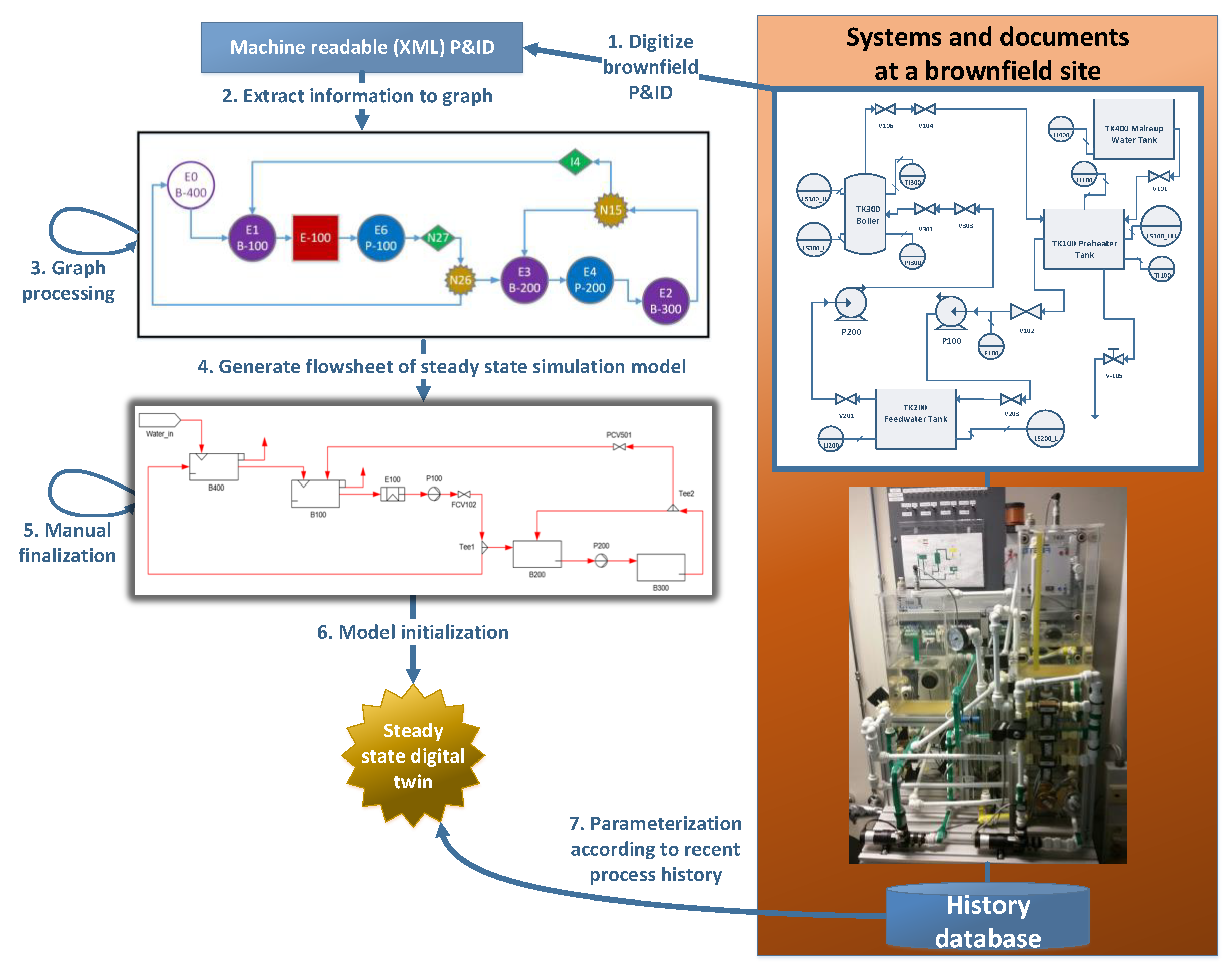
3.1. Methodology Overview

Figure 1 shows a vision for a methodology for the semi-automatic generation of a steady state digital twin for a brownfield process plant. The methodology consists of the following seven steps. Since several research works exist for steps 1 and 2, this article proposes solutions for the remaining steps.
  • The main process design document that is generally available at a brownfield process plant is a P&ID. Some leading P&ID CAD vendor’s tools are able to export P&IDs in a machine readable format according to the standardized Proteus XML schema, but this capability is present only in the most recent tool versions and is thus not applicable to brownfield plants [6,59]. In general, the P&IDs at a brownfield plant are paper documents that have been scanned to pdf-format, so various image recognition techniques are needed to extract information from them [12,48,60,61].
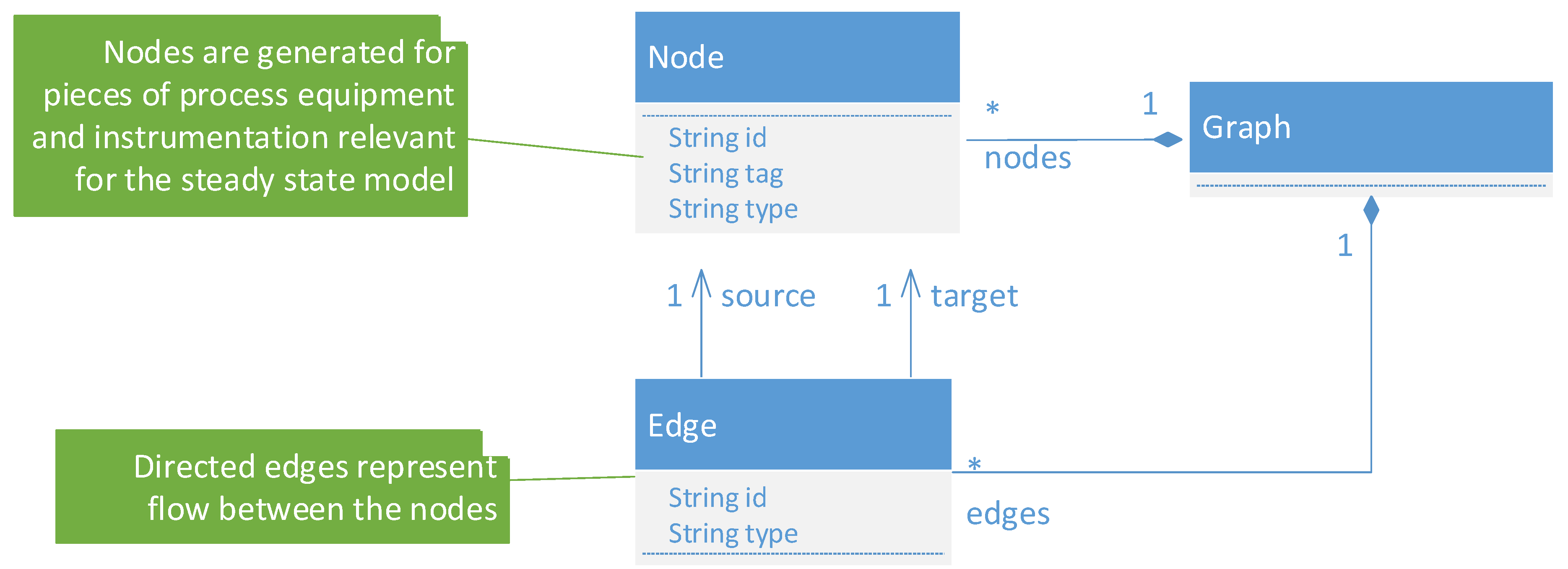
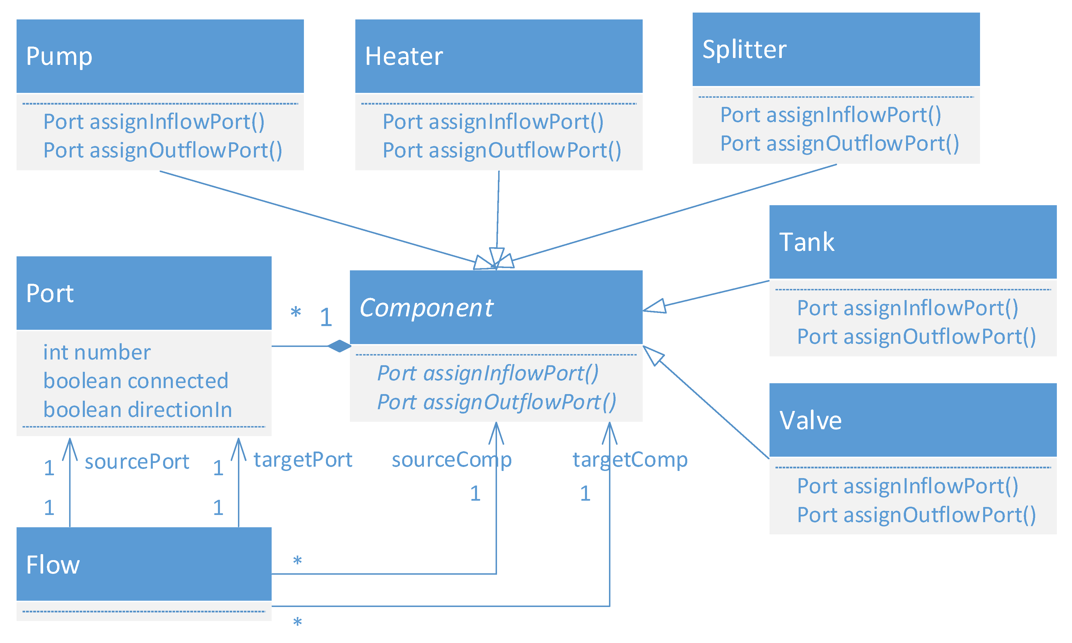
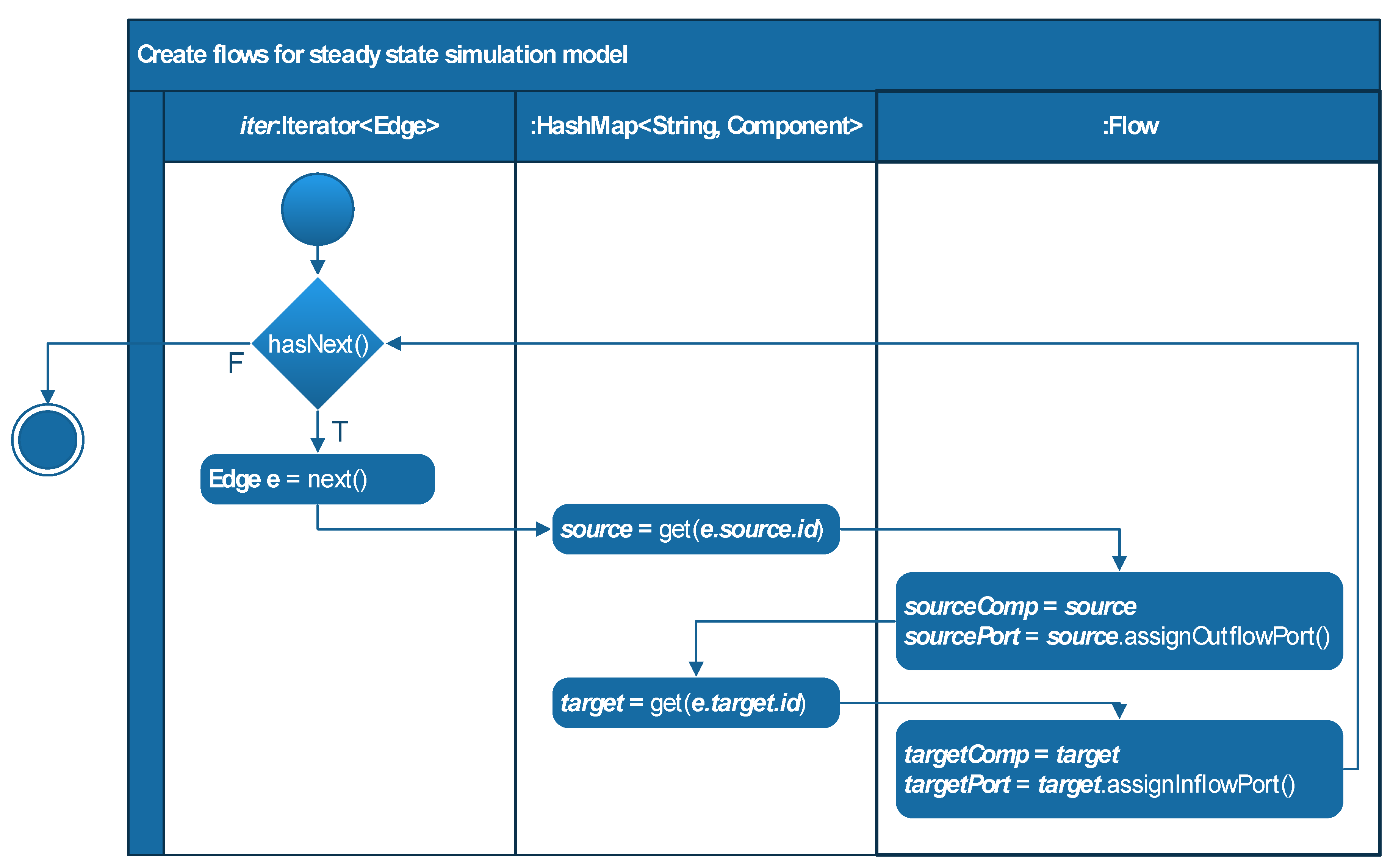
  • Graphs have emerged as an intermediate format for abstracting key information from a process plant design [6,54,55,56]. The information that is relevant for building a steady state simulation model is extracted from the digitalized P&ID into a directed graph, as described in [6]. If Proteus XML is used as the digitalized P&ID format, the methodology will be able to support also modern plants for which the P&ID could be exported directly into this format. However, if the compatibility is not required, any proprietary format for a digitalized P&ID can be used as long as the graph is generated according to the following guidelines. Process equipment such as tanks, pumps, and valves are represented with nodes, and node labels capture the type of the component as well as the tag. Flows are represented with directed edges between the components, and the type of flow (e.g., water or broke) is captured by the edge label.
  • The graph should be transformed until it is at a level of abstraction in which the steady state model can be generated by performing a one-to-one mapping from the graph nodes and edges to the equipment and flows of a steady state model.
  • Simulation tool specific rules should be defined and implemented for generating a flowsheet of the steady state model automatically from the graph generated in step 3. The rules should be implemented by a custom software tool that writes its output into a format that can be imported to the selected simulation tool.
  • A steady state modelling expert should manually finalize the flowsheet of the generated steady state model, using his or her expert modelling knowledge that could not be formalized as rules in step 4.
  • A steady state modelling expert should manually initialize the steady state simulation model by defining the chemical components (i.e., water, pulp, air, steam, etc.) and selecting the calculation modules for each process equipment using his or her expert modelling knowledge that could not be formalized as rules in step 4. Further research could try to automate this step.
  • The selected calculation module defines the needed input values for parameterizing the process equipment. The steady state modelling expert performs the parameterization manually. Further research could try to automate this step. If the parameterization is performed according to recent sensor data from the process, the steady state model may be considered as a digital twin.
This article is scoped as follows. Previous research exists for steps 1 and 2 as has been cited above. This article will provide solutions for steps 3, 4, and 5 and apply them to a case study. Steps 6 and 7 will be addressed as further work in the final section of the article.

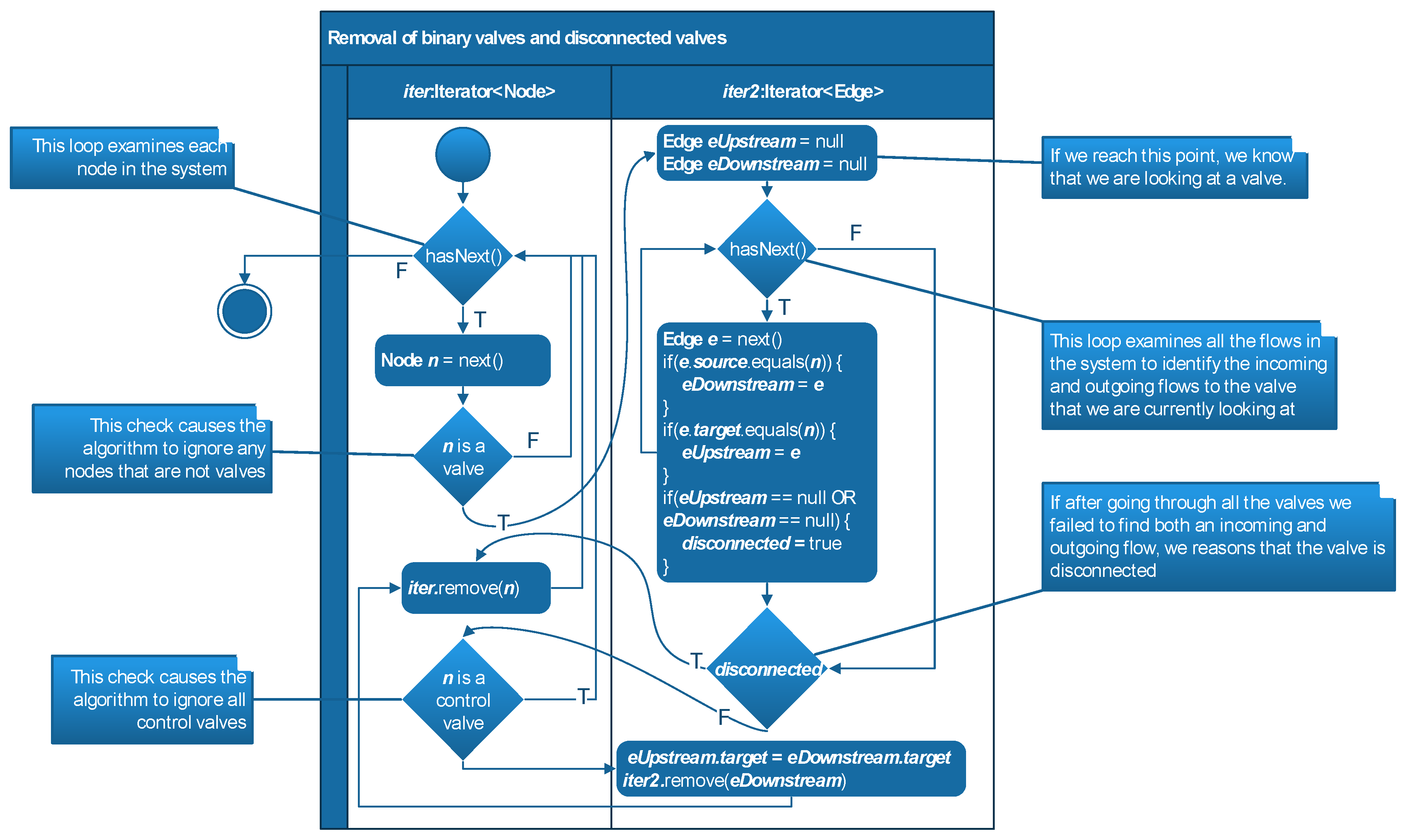
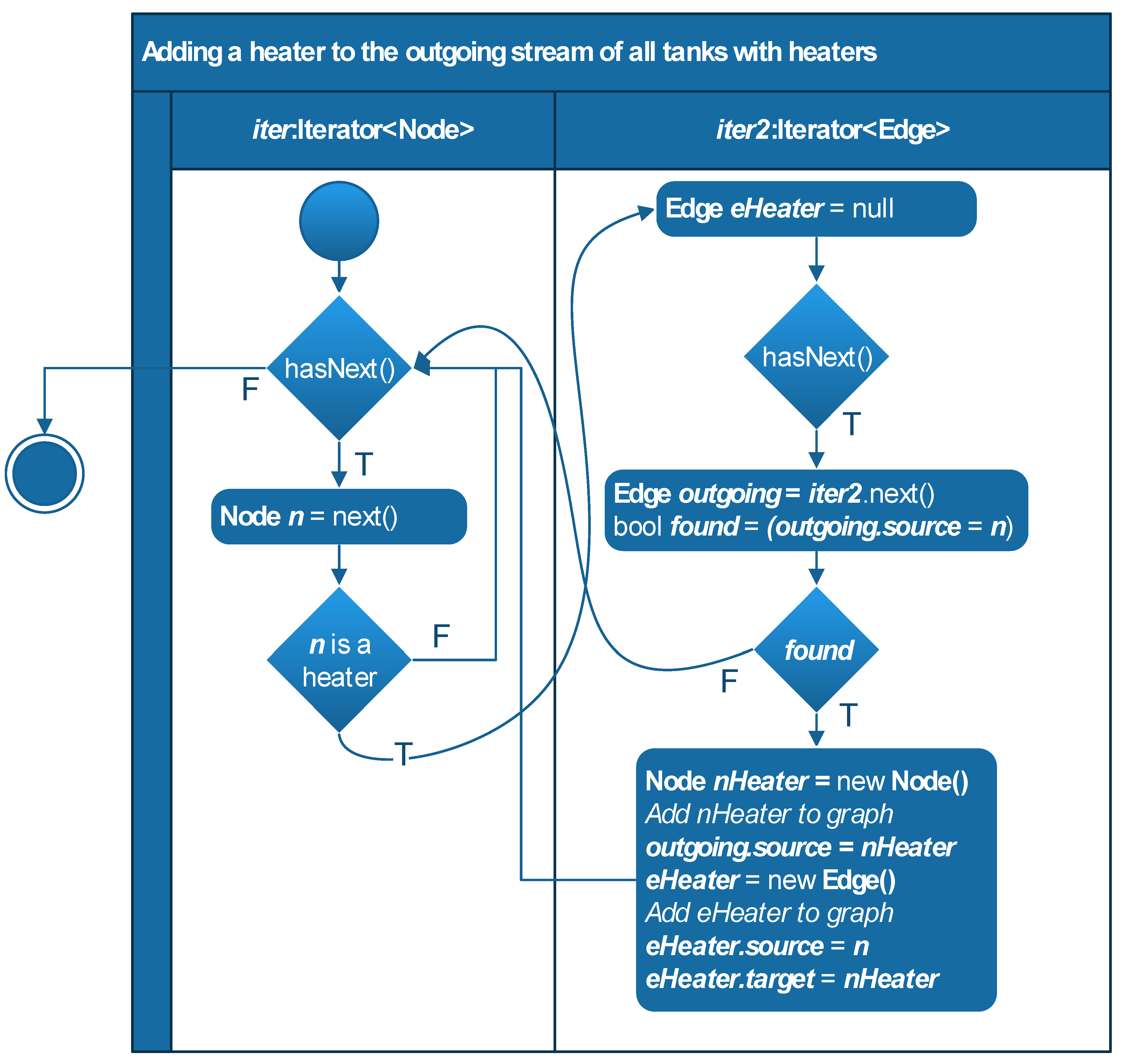
3.2. Graph processing

This section presents algorithms for step 3 of the methodology in Section 3.1. Figure 2 shows a Unified Modeling Language (UML) class diagram of the graph representation of the information extracted from the digitalized P&ID. This methodology assumes that such a graph has been previously generated, e.g., according to the approach presented in [6].
Dynamic modelling captures the time dependency of the process; it predicts all the transient states when the process moves from state A to state B [14]. Thus, the flowsheet of the dynamic simulation model is almost one-to-one with the P&ID including all the control loops with their control and binary valves. Steady state modelling, on the other hand, assumes that all variables are constant in spite of the ongoing process that tends to change them. Thus, the modelling of the binary valves of the control loops is irrelevant and it should not be included in the steady state simulation model. Control valves, on the other hand, are captured in the steady state simulation model to adjust the flows, temperatures, pressures, consistencies, etc. of the steady state. Figure 3, UML activity diagram represenation of an algorithm that removes binary valves from the intermediate graph representation of a process, shows an algorithm for removing the binary valves present in the P&ID from the intermediate graph presentation of the process. The algorithm iterates through all the nodes in the graph and uses node types to identify the binary valves. For each binary valve, the algorithm iterates through all of the edges in the graph to find the edges representing the outgoing and incoming flows of the valve, ‘eDownstream’ and ‘eUpstream’, respectively, in Figure 3. UML activity diagram represenation of an algorithm that removes binary valves from the intermediate graph representation of a process. The node and ‘eDownstream’ are removed. The target of ‘eUpstream’ is changed to the target of ‘eDownstream’.
The binary valve removal algorithm in Figure 3 is relevant for all steady state simulation tools. In contrast, there are differences between how tools model tanks with internal heaters. In some tools, such as the tool used in our case study, the library of equipment symbols does not have a tank with an internal heater. In such cases, the tank with an internal heater can be modelled by adding the heater to the outgoing flow of the tank. Figure 4 shows an activity diagram for this purpose. The source information for this algorithm is the graph outputted by the algorithm in Figure 3, UML activity diagram represenation of an algorithm that removes binary valves from the intermediate graph representation of a process. The algorithm iterates through all nodes in the graph and looks for tanks with heaters (‘heater’ in Figure 4). For all such nodes, the algorithm iterates through all of the edges to find the outgoing edge. A node representing a heating element is added to the outgoing flow.

3.3. Generating a Flowsheet of the Steady State Model

This section presents rules for step 4 of the methodology in Section 3.1. The rules are applied to the intermediate graph outputted by the algorithm in Figure 4. The rules (Table 1) are valid for the selected steady state simulation tool, Balas® (https://info.vttresearch.com/balas). Balas® is a steady state simulation package for chemical processes with emphasis on pulp and paper, food processing and biochemical processes. If another simulation tool was selected, a new set of rules should be created to correspond with the symbols of that simulation tool. Figure 5 presents some symbols in Balas® that are used to simulate different process equipment. Each symbol has one to several ports that are connected to either inlet or outlet streams. The implementation of the rules must ensure that each port of the symbol in the simulation tool is used at most once.
The rules are realized according to the object-oriented paradigm. Figure 6 shows a UML class diagram to capture these structures. Italics in the class diagram denote abstract classes and methods (i.e., the ‘Component’ class and its methods), so all inheriting classes (i.e., ‘Pump’, ‘Heater’, ‘Splitter’, ‘Tank’ and ‘Valve’) must implement these methods. The implementation of these methods should ensure that the ports are assigned according to the rules in Table 1 and that each port is used at most once.
The rules in Table 1 are implemented by algorithms that map the intermediate graph outputted by the algorithm in Figure 4 to the object model in Figure 6. The creation of the various types of components is trivial as the type label of the node is used to determine whether to create an object of type ‘Pump’, ‘Heater’, ‘Splitter’, ‘Tank’ or ‘Valve’. However, the connection of valves to the appropriate ports is not as straightforward. Figure 7 shows an algorithm for this purpose. The algorithm is general in the sense that changes are not required if more component types are added or if the port mapping rules are changed to meet the requirements of a specific steady state simulator. This generality was achieved by using abstraction and inheritance in Figure 6. Any changes are limited to the implementation of the methods ‘assignInflowPort()’ and ‘assignOutflowPort()’.

3.4. Implementation of the Design

The UML designs were implemented as follows in the Java programming language. The composition relation (line with a solid diamond ending) in the class diagrams was implemented with the Java Vector class. For example, the compositions in Figure 2 are implemented with a vector containing elements of type Node and Edge, i.e., Vector<Node> and Vector<Edge>. The iterator() method of these vectors are used to obtain the iterators Iterator<Node> and Iterator<Edge> in Figure 3. The triangular arrows in Figure 6 are generalization relationships. The algorithm in Figure 7 exploits the generalization, so that new component types, such as refiners, columns and reactors, can be added without changes to the algorithm.

4. Case Study

Aalto’s water process plant, which is depicted in Figure 8, consists of different process, electrical, instrumentation and automation components. It can be used for demonstrating various process scenarios and related automation solutions for research and educational purposes. The main task of the plant is to supply heated and pressurized water for a variable load. The return water is reused in a closed-circuit stream. Five main closed control loops are defined to adjust the level of water in the tanks and the temperature and pressure of the supplied load.
The first process component of the closed loop primary stream of the process plant is a Preheater Tank (B-100), which receives the water that is returned from the Supplied Process. In the Preheater Tank, the temperature can be adjusted to the desired temperature by using a heater (E-100), a copper colored component in the bottom right tank in Figure 8. The Preheater Pump (P-100) transfers heated water from the Preheater Tank to the Feedwater Tank (B-200). From there, the Feedwater Pump (P-200) pressurizes the water in the Boiler (B-300) according to a setpoint value, despite disturbances caused by the Supplied Process. A makeup Stream compensates for the loss of water in the primary stream, which occurs gradually over time due to evaporation from the open tanks.
The operator can run the plant in manual or automatic mode; to provide an automatic operation interface, all the sensors and actuators are connected to a remote I/O system, which transfers data between the plant and a soft PLC implemented on a PC. By using OPC UA, the field and automation data can be sent to simulation software like Balas®, Simulink, and Apros.
Figure 9 shows a P&ID of the case process. The P&ID was originally drawn in the SmartPlant P&ID tool but has been redrawn to reduce clutter. The P&ID was exported to Proteus XML using SmartPlant P&ID. The graph in Figure 10 was generated using the methodology in [6]. The graph was processed by the algorithms in Figure 3 and Figure 4. The results are shown in Figure 11 and Figure 12, respectively.
A flowsheet of the steady state model was generated from the graph in Figure 12 using the rules defined in Table 1 and the algorithm in Figure 7. The resulting object model confirming to the class diagram in Figure 6 was serialized to .csv format (Table 2 and Table 3). It is visualized in Figure 13 to help the reader verify that the port numbers and connection conform to the rules in Table 1.
The .csv output was imported to the Balas® steady state simulation tool, resulting in the model in Figure 14. A custom importer plugin was created for a demonstration version of Balas® that is based on Simantics Open operating system for modelling and simulation (https://www.simantics.org/). It uses a graph database for storing simulation models and related data. Simantics provides a general-purpose functional scripting language SCL that is capable of manipulating the models within the database. SCL is also suitable for programming utility functionality on top of released simulation tool products. This version of Balas® includes an IDE for developing and testing SCL-based plugins within the simulator environment. Using SCL APIs for Balas®, a translator function was created that takes as input .csv files and creates corresponding Balas® model structures defined with flowsheet graphics. The importer plugin can in the future be extended to implement automation of steps 6–7 of the methodology.
Step 5 of the methodology in Section 3.1 involves a modeler making manual finalizations to the model in Figure 14 according to expert modelling knowledge that could not be captured as generally valid rules, such as the ones in Table 1. In the selected simulation tool, i.e., Balas®, there are two different kind of calculation modules available for simulating a normal tank.
The more complicated calculation module can be used to simulate a storage tank with several inflows and outflows, an overflow, and a makeup stream. This calculation module is used for simulating buffer tanks. During the simulated steady state, this buffer tank constantly provides a fixed outflow requested by the receiving module located after the buffer tank. If the required amount of flow is not available, the buffer tank provides the missing part through the makeup stream (port #2). The makeup stream may be connected to another tank or e.g., to the freshwater system. If the inflows of the buffer tank exceed the required outflow, the surplus is led to the overflow stream (port #1) which may be connected to another tank or alternatively to the drain. In the case example, the buffer tanks “B400” and “B100” are simulated using this calculation module. The case process is initially filled up with fresh tap water through the makeup stream (“Makeup1”) of the makeup tank “B400”. Also, if there are any leaks in the system, the makeup flow to cover the leaks is taken from the tap water line (“Water in”). The valve “FCV102” is the receiving module that requests a specific flow from the tank “B100”. If the inflow to the tank “B100” from the tank “B300” through the valve “PCV501” is not sufficient, the tank “B100” requests makeup from the makeup tank “B400”, and not from the fresh water system (“Makeup source 2”), as simulated in Figure 12. This change of the makeup stream source was done manually based on the expertise of the modeler.
The simplified calculation module can be used to simulate a storage tank with several inflows and one outflow. The module mixes the inflows together and provides one outflow. This calculation module is used for simulating tanks that during steady state do not have any makeup flow or overflow but rather only a flow-through. In the case process, during steady state, the tanks “B200” and “B300” are such flow-through tanks and can for simplicity be simulated using the more simplified calculation module. These changes of the tank calculation modules (as well as the visual symbol of the tank) for tanks “B200” and “B300” were done manually based on the expertise of the modeler. Figure 15 shows the result of the manual finalizations of the flowsheet presented in Figure 14.
It is very common that the modeler changes the calculation modules for tanks (and the visual symbols presenting the tanks) during the iterative simulation work. In real processes, e.g., in paper machines, the water circuits are very complex connecting several tanks together. The makeup and overflow streams of the tanks are connected across. Some tanks may have a makeup stream from the freshwater system and some overflow streams directed to the sewer. To make a rule for such water circuits would require studying the entire circuit. This is time consuming. Instead, having a rule to model each tank as a complicated one and then later manually simplify the system is faster.
Step 6 of the methodology in Section 3.1 involves the initialization of the model by selecting the chemical components and the calculation modules for the symbols modelling the process equipment in Figure 15.
The initialization of the model starts with selecting manually the chemical components present in the process. In the simulation model, the chemical compositions and the conditions (T,p) of each feed stream must be defined. The chemical compositions of other streams (internal and products) are calculated automatically when the model is run. In the case process, water was the only component present in the feed stream (“Water in”).
After defining the chemical components, the initialization of the model continues with selecting the calculation modules. Each symbol may have one to more calculation modules, which are selected manually in the simulation tool from a drop-down list. For example, the symbol simulating a heater may have a calculation module for either defining the outlet temperature or the thermal duty of the heater. The symbol simulating a valve may have a module for either defining the outlet pressure or the flow through the valve. The splitters may have a module for either defining the true mass flow (kg/s) of the first outlet or the share of the flow to the first outlet. In the case process, the modeler selected the calculation modules manually based on his or her expertise. For example, the calculation module for the heater “E100” was selected to be “the defined outlet temperature”, since the temperature of the water circulating in the case process was known. The calculation module for the valve “FCV102” was selected to be “fixed flow”. This setpoint value sets the amount of the circulating water in the system.
It is typical that during the iterative simulation work, the modeler changes the calculation modules of the symbols depending on what kind of input data (e.g., temperature, thermal duty, flow, etc.) is available.
Step 7 of the methodology in Section 3.1 involves parameterization of the calculation modules for the symbols in Figure 15. The selected calculation module determines the set of input values that are needed to parametrize the module. Possible parameters are, for example, exit pressure (kPa), exit temperature (°C), flow (kg/s), pump efficiency (%) or share of flow to specified stream in a junction. At this point of the research work, the parametrization of the modules was done manually based on the input data available for the case process.
After parametrization, the model can be finally run. Figure 16 shows the results of the simulation model describing the case process. At steady state, there is water circulating through the main line of the system, namely through tanks “B100”, “B200”, and “B300”. Since no leaks are assumed, both the makeup streams have zero flow.

5. Results

The case study has served as a proof-of-concept (POC) to validate the proposed algorithms. The great majority of manual engineering work was automated with respect to generating the flowsheet of the steady state model. It was discovered that all of the work that could not be automated involved the application of expert reasoning that could not readily be captured as general-purpose rules or algorithms. Thus, it was found that the developed approach is not expected to replace the human expert, but rather has potential to increase the engineering productivity of the expert. The findings are insufficient for the purpose of drawing any conclusions about the correctness or extensibility of the proposed algorithms for industrial grade processes. However, the findings about the extent of engineering work that could be automated for this case study indicate that the algorithms are ready for further research in the context of significantly more complex processes.

6. Discussion

The target of the paper was to achieve a POC for the automatic generation of a steady state model. The case process selected for the POC is simple and contains only simple unit operations such as tanks, pumps, and valves that can be modelled in the selected simulation tool with one single symbol. As a result, the rules for a one-to-one mapping from an intermediate graph to a steady state model presented in Table 1 are very simple. For chemical processes with more complicated unit operations, such as distillation columns, evaporators or extractors, the rules are longer since a distillation column or a liquid–liquid extractor, for example, are modelled by combining several symbols in series or parallel instead of having only one symbol. Even though the rule is longer, the same approach is applicable as with the simpler rules presented in this paper. However, further research is needed to define a set of rules to cover the most common chemical unit operations.
If the equipment is not available in the library of the simulation software, it can be modelled by creating a custom combination of equipment available in the library. In the case process, the rules are one-to-one mapping (from one piece of equipment to one symbol in the steady state model). In the said further research on chemical unit operations, several-to-one and/or one-to-several mapping rules are expected. Commercial simulation software may have an emphasis on a certain chemical process technology. For example, the simulation software AspenPlus is powerful for modelling unit operations based on phase separation whereas Balas is designed for modelling and simulating of paper processes. Thus, in AspenPlus there is no single symbol for a headbox of a paper machine and vice versa, in Balas, there is no single symbol for a distillation column. The rule for describing any unit operation is always simulation software specific. In the absence of standardization in the area of steady state simulation tools, one direction for further research would be the development of rules for simulator-to-simulator transfer.
The methodology presented in this paper assumes as its starting point that the relevant information has been extracted from a P&ID into a graph format. For many brownfield plants, the P&ID is a raster graphics image obtained by scanning a paper diagram. In newer plants a digital P&ID from a CAD tool may be available. The latter scenario applies to our case study. Thus, the methodology is general for all kinds of plants. However, it has been especially designed to work on the limited information at a brownfield plant. In the case of raster graphics P&IDs, the quality of the results obtained by this methodology depend additionally on the quality of the P&ID information extraction solution. The availability of recent publications in this area by several research groups, referenced in bullet 1 of the numbered list in Section 3.1, is an indication that efforts are underway to further advance the quality of information extraction from brownfield design documents.

7. Conclusion and Further Work

7.1. Limitations

Flowsheet generation is always a necessary step when building a model. The complexity of generating a flowsheet does not depend on the complexity of the configuration of the process. The flowsheet does not describe the chemical and physical phenomena occurring in the process (i.e., model components and their reactions). The flowsheet describes the connection between the process equipment (i.e., process configuration). The solution presented in this paper is focused on the flowsheet generation. This article has not targeted the information needed to describe thermo-hydraulic or chemical phenomena. To overcome these limitations, it is necessary to (i) select suitable calculation modules, (ii) parametrize the model based on available data and information, and (iii) set the parameter values to the model. The parameters include (i) unit operation input parameters, (ii) feed stream composition and state, (iii) design specification, (iv) solver parameters, and (v) thermodynamic model parametrization. With this information, the flowsheet is supplemented with adequate information of the phenomena and it is possible to simulate the process with the model.

7.2. Summary of Results and Further Work

In this paper, a 7-step methodology was proposed for the generation of steady state digital twins for process plants. Related works were positioned along the steps 1–2, so the focus of the paper was on steps 3–7. The findings and topics of further work for these steps are discussed next.
In our case study, the result of steps 3 and 4 was an automatically generated flowsheet of a steady state model that required only minor manual changes by an expert modeler. Specifically, the following changes were made to two of the tanks: changing the type of the tank to another type of tank from the library of the steady state modelling tool and reconnecting the makeup flows of these tanks. It may be concluded that the generation significantly reduced the manual modelling effort and that the methodology is ready for further research on larger and more complicated processes.
The rationale for the manual changes done in step 5 was presented in detail. The modelling decisions related to a makeup flow of a tank required the consideration of several parts of the process upstream of the said tank. The general formulation of such modelling decisions as rules is a nontrivial problem. However, one direction of further research would be the formulation and implementation of such rules, and validating them across a wide range of case studies.
In step 6, the modelling decisions related to selecting calculation modules were discussed. It was noted that the decisions depend on the properties of incoming flows, which in turn depend on how other parts of the process were modelled. The automation of this work was left for further research.
In step 7, concrete examples of steady state model parameterization were given, and the case model was parameterized manually based on known typical operating parameters of the process. In further work, the developed toolchain could be integrated to the process automation system and its history database in order to retrieve recent sensor values and to use them to automatically parameterize the steady state model. It is proposed that such a capability for automatic parameterization would turn a steady state simulation model to a steady state digital twin. It is notable that there is a lack of research specifically about digital twins based on steady state models, so there is no established definition for a steady state digital twin. Significant further research questions arise related to the development of the automatic parameterization capability, so it is not only an industrial information integration task. Knowledge about the recent operating conditions of the process is required to select and preprocess a suitable time period of recent process history, in order to parameterize a steady state model that will be relevant for answering the specific questions related to the unique retrofit project at hand.

Author Contributions

Conceptualization, S.S., L.S., and M.A.; Data curation, S.S. and L.S.; Formal analysis, S.S. and L.S.; Funding acquisition, S.S. and E.H.; Investigation, S.S.; Methodology, S.S. and L.S.; Project administration, S.S. and E.H.; Resources, S.S., L.S., and V.V.; Software, S.S. and A.V.; Supervision, S.S., E.H., and V.V.; Validation, S.S., L.S., and A.V.; Visualization, S.S. and M.A. Writing—original draft, S.S., L.S., M.A., and A.V.; Writing—review & editing, S.S., L.S., M.A., E.H., and V.V. All authors have read and agreed to the published version of the manuscript.

Funding

This research was funded by Business Finland grants 3915/31/2019 and 4153/31/2019.

Conflicts of Interest

The authors declare no conflict of interest. The funder had no role in the design of the study; in the collection, analyses, or interpretation of data; in the writing of the manuscript, or in the decision to publish the results.

References

  1. Pinto-Varela, T.; Barbosa-Póvoa, A.P.F.D.; Carvalho, A. Sustainable batch process retrofit design under uncertainty—An integrated methodology. Comput. Chem. Eng. 2017, 102, 226–237. [Google Scholar] [CrossRef]
  2. Wang, B.; Klemeš, J.J.; Varbanov, P.S.; Chin, H.H.; Wang, Q.-W.; Zeng, M. Heat exchanger network retrofit by a shifted retrofit thermodynamic grid diagram-based model and a two-stage approach. Energy 2020, 198, 117338. [Google Scholar] [CrossRef]
  3. Min, K.-J.; Binns, M.; Oh, S.-Y.; Cha, H.-Y.; Kim, J.-K.; Yeo, Y.-K. Screening of site-wide retrofit options for the minimization of CO2 emissions in process industries. Appl. Therm. Eng. 2015, 90, 335–344. [Google Scholar] [CrossRef]
  4. Faria, D.C.; Bagajewicz, M.J. Profit-based grassroots design and retrofit of water networks in process plants. Comput. Chem. Eng. 2009, 33, 436–453. [Google Scholar] [CrossRef]
  5. Wen, M.; Wu, Q.; Li, G.; Wang, S.; Li, Z.; Tang, Y.; Xu, L.; Liu, T. Impact of ultra-low emission technology retrofit on the mercury emissions and cross-media transfer in coal-fired power plants. J. Hazard. Mater. 2020, 396, 122729. [Google Scholar] [CrossRef] [PubMed]
  6. Sierla, S.; Azangoo, M.; Vyatkin, V.; Fay, A.; Papakonstantinou, N. Integrating 2D and 3D Digital Plant Information towards Automatic Generation of Digital Twins. In Proceedings of the 29th IEEE International Symposium on Industrial Electronics, Delft, The Netherlands, 17–19 June 2020. [Google Scholar]
  7. Chen, B.; Wan, J.; Shu, L.; Li, P.; Mukherjee, M.; Yin, B. Smart Factory of Industry 4.0: Key Technologies, Application Case, and Challenges. IEEE Access 2018, 6, 6505–6519. [Google Scholar] [CrossRef]
  8. Schluse, M.; Priggemeyer, M.; Atorf, L.; Roßmann, J.; Romann, J. Experimentable Digital Twins—Streamlining Simulation-Based Systems Engineering for Industry 4.0. IEEE Trans. Ind. Inform. 2018, 14, 1722–1731. [Google Scholar] [CrossRef]
  9. Martinez, G.S.; Karhela, T.A.; Ruusu, R.J.; Sierla, S.; Vyatkin, V. An Integrated Implementation Methodology of a Lifecycle-Wide Tracking Simulation Architecture. IEEE Access 2018, 6, 15391–15407. [Google Scholar] [CrossRef]
  10. Martinez, G.S.; Sierla, S.; Karhela, T.; Lappalainen, J.; Vyatkin, V. Automatic Generation of a High-Fidelity Dynamic Thermal-Hydraulic Process Simulation Model from a 3D Plant Model. IEEE Access 2018, 6, 45217–45232. [Google Scholar] [CrossRef]
  11. Martínez, G.S.; Sierla, S.; Karhela, T.; Vyatkin, V. Automatic Generation of a Simulation-Based Digital Twin of an Industrial Process Plant. In Proceedings of the 44th Annual Conference of the IEEE Industrial Electronics Society IECON 2018, Washington, DC, USA, 21–23 October 2018; pp. 3084–3089. [Google Scholar] [CrossRef] [Green Version]
  12. Arroyo, E.; Hoernicke, M.; Rodríguez, P.; Fay, A. Automatic derivation of qualitative plant simulation models from legacy piping and instrumentation diagrams. Comput. Chem. Eng. 2016, 92, 112–132. [Google Scholar] [CrossRef]
  13. Shellshear, E.; Berlin, R.; Carlson, J.S. Maximizing Smart Factory Systems by Incrementally Updating Point Clouds. IEEE Comput. Graph. Appl. 2015, 35, 62–69. [Google Scholar] [CrossRef] [PubMed]
  14. Emerson. Understanding and Applying Simulation Fidelity to the Digital Twin. White Paper 2018. Available online: emerson.com/documents/automation/understanding-applying-simulation-fidelity-to-digital-twin-en-5079366 (accessed on 2 October 2020).
  15. Matzopoulos, M. Dynamic Process Modeling: Combining Models and Experimental Data to Solve Industrial Problems. In Process Systems Engineering: Volume 7 Dynamic Process Modeling; Georgiadis, M.C., Banga, J.R., Pistikopoulos, E.N., Eds.; Wiley-VCH: Weinheim, Germany, 2010; pp. 1–33. [Google Scholar] [CrossRef]
  16. Leiviskä, K. Simulation in Pulp and Paper Industry; University of Oulu, Control Engineering Laboratory: Oulu, Finland, 1996; Report A, 2; pp. 1–58. [Google Scholar]
  17. Blanco, A.; Dahlquist, E.; Kappen, J.; Manninen, J.; Negro, C.; Ritala, R. Use of modelling and simulation in the pulp and paper industry. Math. Comput. Model. Dyn. Syst. 2009, 15, 409–423. [Google Scholar] [CrossRef]
  18. Bezzo, F.; Bernardi, R.; Cremonese, G.; Finco, M.; Barolo, M. Using Process Simulators for Steady-State and Dynamic Plant Analysis. Chem. Eng. Res. Des. 2004, 82, 499–512. [Google Scholar] [CrossRef]
  19. Enaasen, N.; Tobiesen, A.; Kvamsdal, H.M.; Hillestad, M. Dynamic Modeling of the Solvent Regeneration Part of a CO2 Capture Plant. Energy Procedia 2013, 37, 2058–2065. [Google Scholar] [CrossRef] [Green Version]
  20. Măluțan, T.; Mǎluţan, C. Simulation of Processes in Papermaking by WinGEMS Software. Environ. Eng. Manag. J. 2013, 12, 1645–1647. [Google Scholar] [CrossRef]
  21. Turon, X.; Labidi, J.; Paris, J. Simulation and optimisation of a high grade coated paper mill. J. Clean. Prod. 2005, 13, 1424–1433. [Google Scholar] [CrossRef]
  22. Cardoso, M.; De Oliveira, K.D.; Costa, G.A.A.; Passos, M.L. Chemical process simulation for minimizing energy consumption in pulp mills. Appl. Energy 2009, 86, 45–51. [Google Scholar] [CrossRef]
  23. Atkins, M.; Morrison, A.; Walmsley, M.; Riley, J. WinGEMS Modelling and Pinch Analysis of a Paper Machine for Utility Reduction. Appita J. 2010, 63, 281–287. [Google Scholar]
  24. Jönsson, J.; Ruohonen, P.; Michel, G.; Berntsson, T. The potential for steam savings and implementation of different biorefinery concepts in Scandinavian integrated TMP and paper mills. Appl. Therm. Eng. 2011, 31, 2107–2114. [Google Scholar] [CrossRef] [Green Version]
  25. Clement, S.; Gouiller, A.; Ottenio, P.; Nivelon, S.; Huber, P.; Nortier, P. Speciation and supersaturation model in papermaking streams. Process. Saf. Environ. Prot. 2011, 89, 67–73. [Google Scholar] [CrossRef]
  26. Huber, P.; Nivelon, S.; Ottenio, P.; Nortier, P. Coupling a Chemical Reaction Engine with a Mass Flow Balance Process Simulation for Scaling Management in Papermaking Process Waters. Ind. Eng. Chem. Res. 2012, 52, 421–429. [Google Scholar] [CrossRef]
  27. Kangas, P.; Kaijaluoto, S.; Määttänen, M. Evaluation of future pulp mill concepts—Reference model of a modern Nordic kraft pulp mill. Nord. Pulp Pap. Res. J. 2014, 29, 620–634. [Google Scholar] [CrossRef]
  28. Barbera, E.; Menegon, S.; Banzato, D.; D’Alpaos, C.; Bertucco, A. From biogas to biomethane: A process simulation-based techno-economic comparison of different upgrading technologies in the Italian context. Renew. Energy 2019, 135, 663–673. [Google Scholar] [CrossRef]
  29. Kautto, J.; Realff, M.J.; Ragauskas, A.J. Design and simulation of an organosolv process for bioethanol production. Biomass Convers. Biorefinery 2013, 3, 199–212. [Google Scholar] [CrossRef]
  30. Søtoft, L.F.; Rong, B.-G.; Christensen, K.; Norddahl, B. Process simulation and economical evaluation of enzymatic biodiesel production plant. Bioresour. Technol. 2010, 101, 5266–5274. [Google Scholar] [CrossRef]
  31. Cheah, K.W.; Yusup, S.; Singh, H.K.G.; Uemura, Y.; Lam, H.L.; Wai, C.K. Process simulation and techno economic analysis of renewable diesel production via catalytic decarboxylation of rubber seed oil—A case study in Malaysia. J. Environ. Manag. 2017, 203, 950–961. [Google Scholar] [CrossRef]
  32. Barbosa, L.D.S.N.S.; Hytönen, E.; Vainikka, P. Carbon mass balance in sugarcane biorefineries in Brazil for evaluating carbon capture and utilization opportunities. Biomass Bioenergy 2017, 105, 351–363. [Google Scholar] [CrossRef]
  33. Hytönen, E.; Stuart, P.R. Biofuel Production in an Integrated Forest Biorefinery—Technology Identification under Uncertainty. J. Biobased Mater. Bioenergy 2010, 4, 58–67. [Google Scholar] [CrossRef]
  34. Nabgan, B.; Abdullah, T.A.T.; Nabgan, W.; Ahmad, A.; Saeh, I.; Moghadamian, K. Process Simulation for Removing Impurities from Wastewater Using Sour Water 2-Strippers system via Aspen Hysys. Chem. Prod. Process. Model. 2016, 11, 315–321. [Google Scholar] [CrossRef]
  35. Miltner, A.; Wukovits, W.; Pröll, T.; Friedl, A. Renewable hydrogen production: A technical evaluation based on process simulation. J. Clean. Prod. 2010, 18, S51–S62. [Google Scholar] [CrossRef]
  36. Zhang, Y.; Cruz, J.; Zhang, S.; Lou, H.H.; Benson, T.J. Process simulation and optimization of methanol production coupled to tri-reforming process. Int. J. Hydrogen Energy 2013, 38, 13617–13630. [Google Scholar] [CrossRef]
  37. Michaux, B.; Rudolph, M.; Reuter, M.A.; Reuter, M.A. Study of process water recirculation in a flotation plant by means of process simulation. Miner. Eng. 2020, 148, 106181. [Google Scholar] [CrossRef]
  38. McNulty, M.J.; Gleba, Y.; Tusé, D.; Hahn-Löbmann, S.; Giritch, A.; Nandi, S.; McDonald, K.A. Techno-economic analysis of a plant-based platform for manufacturing antimicrobial proteins for food safety. Biotechnol. Prog. 2019, 36, e2896. [Google Scholar] [CrossRef] [PubMed]
  39. Bon, J.; Clemente, G.; Váquiro, H.; Mulet, A. Simulation and optimization of milk pasteurization processes using a general process simulator (ProSimPlus). Comput. Chem. Eng. 2010, 34, 414–420. [Google Scholar] [CrossRef]
  40. Koulamas, C.; Kalogeras, A.P. Cyber-Physical Systems and Digital Twins in the Industrial Internet of Things. Computer 2018, 51, 95–98. [Google Scholar] [CrossRef]
  41. Tao, F.; Zhang, M. Digital Twin Shop-Floor: A New Shop-Floor Paradigm towards Smart Manufacturing. IEEE Access 2017, 5, 20418–20427. [Google Scholar] [CrossRef]
  42. Zhang, H.; Liu, Q.; Chen, X.; Zhang, D.; Leng, J. A Digital Twin-Based Approach for Designing and Multi-Objective Optimization of Hollow Glass Production Line. IEEE Access 2017, 5, 26901–26911. [Google Scholar] [CrossRef]
  43. Wan, J.; Tang, S.; Li, D.; Imran, M.; Zhang, C.; Liu, C.; Pang, Z. Reconfigurable Smart Factory for Drug Packing in Healthcare Industry 4.0. IEEE Trans. Ind. Inform. 2018, 15, 507–516. [Google Scholar] [CrossRef]
  44. Schmidt, N.; Lüder, A. The Flow and Reuse of Data: Capabilities of Automation ML in the Production System Life Cycle. IEEE Ind. Electron. Mag. 2018, 12, 59–63. [Google Scholar] [CrossRef]
  45. Hartmann, B.; Török, S.; Börcsök, E.; Groma, V.O. Multi-objective method for energy purpose redevelopment of brownfield sites. J. Clean. Prod. 2014, 82, 202–212. [Google Scholar] [CrossRef]
  46. Sørensen, D.; Brunoe, T.D.; Nielsen, K. Brownfield Development of Platforms for Changeable Manufacturing. Procedia CIRP 2019, 81, 986–991. [Google Scholar] [CrossRef]
  47. Illa, P.K.; Padhi, N. Practical Guide to Smart Factory Transition Using IoT, Big Data and Edge Analytics. IEEE Access 2018, 6, 55162–55170. [Google Scholar] [CrossRef]
  48. Barth, M.; Fay, A. Automated generation of simulation models for control code tests. Control. Eng. Pract. 2013, 21, 218–230. [Google Scholar] [CrossRef]
  49. Stojanovic, N.; Milenovic, D. Data-driven Digital Twin approach for process optimization: An industry use case. In Proceedings of the 2018 IEEE International Conference on Big Data (Big Data), Seattle, WA, USA, 10–13 December 2018; pp. 4202–4211. [Google Scholar]
  50. Makarov, V.; Frolov, Y.; Parshina, I.S.; Ushakova, M. The Design Concept of Digital Twin. In Proceedings of the 2019 Twelfth International Conference “Management of large-scale system development” (MLSD), Moscow, Russia, 1–3 October 2019; pp. 1–4. [Google Scholar]
  51. Kychkin, A.; Nikolaev, A. IoT-based Mine Ventilation Control System Architecture with Digital Twin. In Proceedings of the 2020 International Conference on Industrial Engineering, Applications and Manufacturing (ICIEAM), Sochi, Russia, 18–22 May 2020; pp. 1–5. [Google Scholar]
  52. Barth, M.; Strube, M.; Fay, A.; Weber, P.; Greifeneder, J. Object-oriented engineering data exchange as a base for automatic generation of simulation models. In Proceedings of the 2009 35th Annual Conference of IEEE Industrial Electronics, Porto, Portugal, 3–5 November 2009; pp. 2465–2470. [Google Scholar]
  53. Campos, J.G.; López, J.S.; Quiroga, J.I.A.; Seoane, A.M.E. Automatic generation of digital twin industrial system from a high level specification. Procedia Manuf. 2019, 38, 1095–1102. [Google Scholar] [CrossRef]
  54. Sierla, S.; Azangoo, M.; Vyatkin, V. Generating an Industrial Process Graph from 3D Pipe Routing Information. In Proceedings of the 25th IEEE International Conference on Emerging Technologies and Factory Automation, ETFA 2020, Vienna, Austria, 8–11 September 2020. [Google Scholar]
  55. Wen, R.; Tang, W.; Su, Z. Topology based 2D engineering drawing and 3D model matching for process plant. Graph. Model. 2017, 92, 1–15. [Google Scholar] [CrossRef]
  56. Rantala, M.; Niemistö, H.; Karhela, T.; Sierla, S.; Vyatkin, V. Applying graph matching techniques to enhance reuse of plant design information. Comput. Ind. 2019, 107, 81–98. [Google Scholar] [CrossRef]
  57. Son, H.; Kim, C.; Kim, C. 3D reconstruction of as-built industrial instrumentation models from laser-scan data and a 3D CAD database based on prior knowledge. Autom. Constr. 2015, 49, 193–200. [Google Scholar] [CrossRef]
  58. Lee, J.; Son, H.; Kim, C.; Kim, C. Skeleton-based 3D reconstruction of as-built pipelines from laser-scan data. Autom. Constr. 2013, 35, 199–207. [Google Scholar] [CrossRef]
  59. Papakonstantinou, N.; Karttunen, J.; Sierla, S.; Vyatkin, V. Design to automation continuum for industrial processes: ISO 15926–IEC 61131 versus an industrial case. In Proceedings of the 2019 24th IEEE International Conference on Emerging Technologies and Factory Automation (ETFA), Zaragoza, Spain, 10–13 September 2019; pp. 1207–1212. [Google Scholar]
  60. Sinha, A.; Bayer, J.; Bukhari, S.S. Table Localization and Field Value Extraction in Piping and Instrumentation Diagram Images. In Proceedings of the 2019 International Conference on Document Analysis and Recognition Workshops (ICDARW), Sydney, Australia, 20–25 September 2019; Volume 1, pp. 26–31. [Google Scholar]
  61. Nurminen, J.K.; Rainio, K.; Numminen, J.P.; Syrjänen, T.; Paganus, N.; Honkoila, K. Object Detection in Design Diagrams with Machine Learning. In Advances in Intelligent Systems and Computing; Springer: Cham, Germany, 2020; Volume 977, pp. 27–36. [Google Scholar] [CrossRef]
Figure 1. Proposed methodology for the semi-automatic generation of a steady state digital twin for a brownfield plant.
Applsci 10 06959 g001
Figure 2. UML class diagram of the graph representation of the information extracted from the digitalized P&ID.
Applsci 10 06959 g002
Figure 3. UML activity diagram represenation of an algorithm that removes binary valves from the intermediate graph representation of a process.
Applsci 10 06959 g003
Figure 4. A UML activity diagram representation of an algorithm for manipulating heating elements in the intermediate graph.
Applsci 10 06959 g004
Figure 5. Different symbols in the Balas® simulation software for simulating process equipment.
Applsci 10 06959 g005
Figure 6. UML class diagram of the steady state model structure.
Applsci 10 06959 g006
Figure 7. UML activity diagram representation of an algorithm that creates the flows and connects them to the correct ports according to the mapping rules in Table 1.
Applsci 10 06959 g007
Figure 8. Aalto’s water process plant.
Applsci 10 06959 g008
Figure 9. P&ID of the case process.
Applsci 10 06959 g009
Figure 10. Graph representation of the information extracted from the digitalized P&ID.
Applsci 10 06959 g010
Figure 11. The result of processing the graph in Figure 10 with the algorithm in Figure 3. All binary valves are removed.
Applsci 10 06959 g011
Figure 12. The result of processing the graph in Figure 11 with the algorithm in Figure 4. The tank with an internal heater is presented by adding the heater to the outgoing flow of the tank.
Applsci 10 06959 g012
Figure 13. Visualization of the Balas® model specified in Table 2 and Table 3.
Applsci 10 06959 g013
Figure 14. Imported flowsheet of the steady state model.
Applsci 10 06959 g014
Figure 15. Final flowsheet of the steady state model resulting from expert manual finalizations of the model in Figure 14.
Applsci 10 06959 g015
Figure 16. Simulations results of the case process.
Applsci 10 06959 g016
Table 1. Rules for a one-to-one mapping from an intermediate graph to a steady state model.
Graph StructureMapping to Balas®
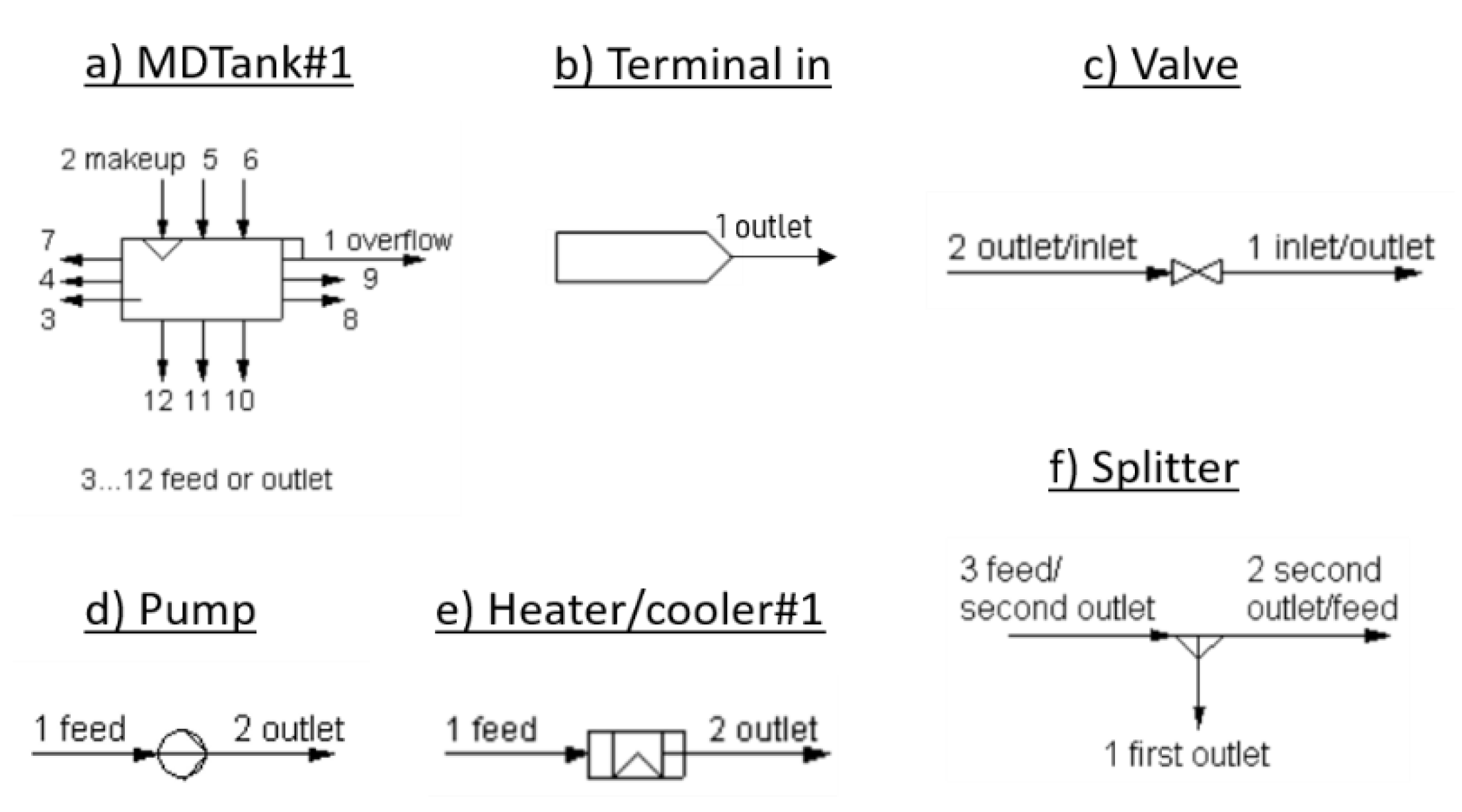
A node of type tank, with one outgoing edge and one or more incoming edgesReplace all tank nodes with a symbol “MDTank#1” (See Figure 5a). Add a stream from port#1 of symbol “Terminal in” (See Figure 5b) to port #2 of symbol “MDTank#1”. From port #1 of symbol “MDTank#1”, add a stream to nowhere. Ports #3-#12 of the symbol “MDTank#1” can be used either for feed or outlet.
A node of type valve, pump or heater with one incoming and one outgoing edgeThe relevant symbols are “Valve” (See Figure 5c), “Pump” (See Figure 5d), “Heater/cooler#1” (See Figure 5e). For each of these symbols, port #1 is for inlet and port #2 is for outlet.
A node of type tee with one incoming and two outgoing edgesReplace tees with symbol “Splitter” (See Figure 5f) with port #3 for inlet and ports #1 and #2 for outlet.
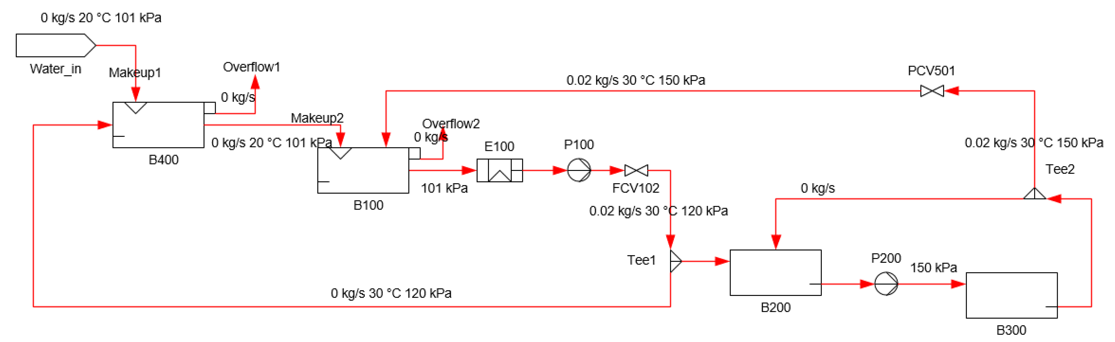
Table 2. Components (i.e., symbol in Balas®) of the steady state model
NodeNameSymbol
B-400MDTank#1
Source1Terminal in
B-100MDTank#1
Source2Terminal in
B-300MDTank#1
Source3Terminal in
B-200MDTank#1
Source4Terminal in
P-200Pump
P-100Pump
I4Valve
ES-E100Heater/cooler#1
N15Splitter
N26Splitter
N27Valve
Table 3. Flows of the steady state model. The strings in ‘Source’ and ‘Target’ columns refer to symbol names in the ‘NodeName’ column of Table 2.
SourceSourcePortTargetTargetPort
Source11B-4002
B-4001drain0
Source21B-1002
B-1001drain0
Source31B-3002
B-3001drain0
Source41B-2002
B-2001drain0
B-2003P-2001
B-4003B-1003
I42B-1004
N151I41
B-3003N153
N152B-2004
P-1002N271
N272N263
N261B-2005
N262B-4004
ES-E1002P-1001
P-2002B-3004
B-1005ES-E1001

