Modeling the Drying of Capillary-Porous Materials in a Thin Layer: Application to the Estimation of Moisture Content in Thin-Walled Building Blocks

Abstract

Drying, as a process of changing the moisture content and temperature of capillary-porous materials, is a necessary step in many technologies. When predicting moisture changes, it is necessary to find a balance between the complexity of a model and the accuracy of the simulation results. The purpose of this work was the development of a mathematical model for drying a capillary-porous material with direct consideration of its initial moisture content and drying temperature. Methods of mathematical modeling were used in the work. Using the developed model, an analysis of the features of the drying process of materials with high and low initial moisture content has been carried out. The analytical relationship for determining the time at which the extremum of the drying rate is reached has been substantiated. A model has been developed to directly take into account the influence of the initial material moisture content and drying temperature. The simulation results are consistent with the experiments on drying ceramic blocks for construction which are described in the literature. The obtained results can be taken into account in studies of the effect of drying modes on the energy consumption of a drying process.

1. Introduction

Drying is a necessary step in many technological processes for processing capillary-porous organic and inorganic materials. From a physical point of view, drying is a process of heat and mass transfer, the result of which is a decrease in the liquid content of a material. This liquid can be organic solvents, but most often it is water. There are many known drying methods. However, in any case, a significant input of heat and time is required to carry out the drying. With an increase in the drying temperature, the time spent decreases, but the energy consumption for heat production increases. If drying is carried out under natural conditions, then the duration of this process may be unacceptably long. On the other hand, excessively high drying temperatures can lead to a decrease in product quality. In order to reduce the time and energy consumption, methods of drying the material in a thin layer are often used, which has been studied in a large number of works [1,2,3]. This drying method is discussed in this paper.

Note that in addition to forced drying in artificial conditions, drying in natural conditions is also used [4]. The elements of wooden roofs function in conditions of cyclical effects of natural drying and humidification [5,6,7], for the diagnosis of which the considered models can be used. The same models can be adapted as a tool for studying the life cycle of building materials [8,9], thermal insulation materials and wall structures [10], as a contribution to achieving the main goal of sustainable development.

The problem is that drying of capillary-porous materials is a complex phenomenon [11,12,13,14,15,16], but practice requires simple methods to predict and optimize drying time and temperature quite accurately. Tests of real materials and structures are expensive. Therefore, it is recommended to predict the drying process using mathematical models [1,12,13].

Reviews of drying models in a thin layer are given in [17] (analysis of five models published from 1921 to 1978), [14] (review of 14 models), [15] (six models considered), [1] (67 models from 2003 to 2013), [16] (10 models from 2013 to 2019). Models of material drying in a thin layer allow predicting the moisture content of the material depending on the drying time, while not requiring complex calculations. For example [15], a Page model M_R = exp(−ktⁿ) with two parameters, in which t—drying time, k and n—empirical constants (parameters), is often used as one of the best in terms of accuracy and analytical simplicity [1,17]. However, this model does not formally reproduce the explicit (separate) effect of the initial moisture content and the drying temperature of the material in the above calculation formula. Initial moisture content and temperature are taken into account indirectly using the parameters k and n. In other words, the influence of the initial moisture content and drying temperature is indistinguishable and aggregated in the parameters k and n along with the influence of the structural features of the capillary-porous medium and other factors. For example, the values k and n in modeling the drying of a capillary-porous material with a thickness of 25 mm, considered in [15] (Table 3), were taken equal to 0.0474 and 1.67 (T = 343 K), respectively; 0.217 and 1.50 (T = 373 K); 0.503 and 1.40 (T = 393 K). Obviously, the decomposition of parameters k and n, i.e., separate consideration of the influence of the initial moisture content of the material and the drying temperature, will expand the predictive capabilities of the model, which will make it possible to better understand the characteristics of drying various materials and increase their competitiveness. The implementation of this predictive capability is investigated in the article using the example of Newton’s model.

In logical connection with the above brief analysis, the purpose of this work is determined: to develop a mathematical model for drying a capillary-porous material with direct consideration of its initial moisture content and drying temperature, including indirect consideration of other factors.

2. Materials and Methods

In accordance with the above purpose, the development of the model was carried out using mathematical modeling methods. For the theoretical substantiation of the drying model, an approach was modified, a simplified version of which is known from [18]. Let us consider the basic concepts and definitions necessary for building a model from a methodological point of view.

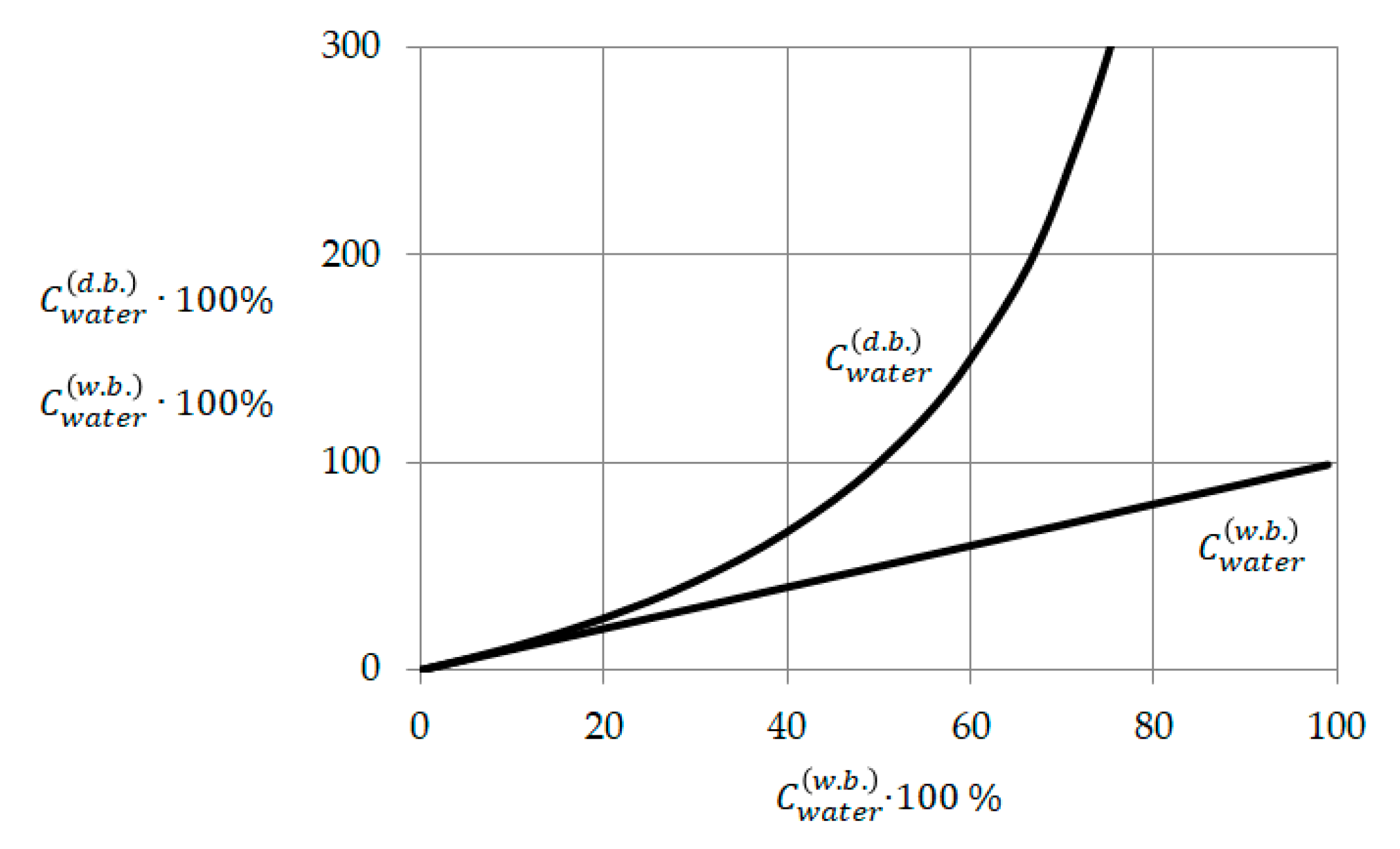
2.1. Main Concepts and Definitions

Let a capillary-porous material of mass $M$ contain a dry matter of mass M_dry and water of mass M_water:

$$M=M_{dry}+M_{water}$$

(1)

The ratio of M_dry and M_water depends on the processes of interaction with the environment. Obviously M_dry/M + M_water/M = 1. According to the physical meaning, M_dry/M—the concentration of dry matter, M_water/M—the concentration of water in the capillary-porous material (by weight).

Based on the fact that the test material with mass M contains water, it is logical to call the ratio M_water/M—the moisture content of the material, determined on a wet basis (w.b.). Accordingly, the ratio M_dry/M determines the dry matter concentration on the same basis (w.b.). Let us denote:

$$C_{water}^{(w.b.)}=\frac{M_{water}}{M}$$

(2)

$$C_{dry}^{(w.b.)}=\frac{M_{dry}}{M}$$

(3)

In the literature, dry basis moisture content (or d.b.) $C_{water}^{(d.b.)}$ is often used as dimensionless characteristics of the state of a capillary-porous material. By analogy with [19,20,21], we write:

$$C_{water}^{(d.b.)}=\frac{M_{water}}{M_{dry}}$$

(4)

Characteristics (2), (3) and (4) are interval variables:

$$0<C_{water}^{(w.b.)}<1, 0<C_{dry}^{(w.b.)}<1$$

(5)

$$0<C_{water}^{(d.b.)}<\infty$$

(6)

The relation between $C_{water}^{(w.b.)}$ and $C_{water}^{(d.b.)}$ is found using (2) and (4). For this, taking into account Equation (1), we write the equality $C_{water}^{(w.b.)}M=C_{water}^{(w.b.)}\left(M_{dry}+M_{water}\right)$ and divide both of its parts by M_dry. Taking into account (4), we get:

$$C_{water}^{(w.b.)}=\frac{C_{water}^{(d.b.)}}{1+C_{water}^{(d.b.)}}$$

(7)

Equation (7) implies that $C_{water}^{(w.b.)}$ ≤ $C_{water}^{(d.b.)}$.

Using (7), we find

$$C_{water}^{(d.b.)}=\frac{C_{water}^{(w.b.)}}{1-C_{water}^{(w.b.)}}$$

(8)

Figure 1 illustrates the relationship between $C_{water}^{(w.b.)}$ and $C_{water}^{(d.b.)}$. Note that if the moisture content of the material is low (≤0.2), then $C_{water}^{(w.b.)}$ ≈ $C_{water}^{(d.b.)}$.

Relations (5) and (6), as well as Figure 1 suggest that it is easier to use $C_{water}^{(w.b.)}$ from Equation (2) as an indicator of moisture in a theoretical study.

2.2. Substantiation of the Model

Let us consider a sample of a capillary-porous material of mass M (1). Drying is performed at a temperature T °C. Over time t, due to a decrease in the moisture content of the material, the values M_water and M decrease by the same value ΔM_water. Then at the moments of time t and $\tilde{t}=t+\Delta t$, the mass of moisture is M_water and (M_water − ΔM_water), respectively; the mass of a sample at the same times is equal to M and (M − ΔM_water). At the same moments of time, relative moisture content (2) is determined by relations (9) and (10), respectively:

$$C_{water}^{(w.b.)}=\frac{M_{water}}{M}$$

(9)

$${\tilde{C}}_{water}^{(w.b.)}=\frac{M_{water}-\Delta M_{water}}{M-\Delta M_{water}}$$

(10)

For a sufficiently small value of Δt, we can assume that the value of ΔM_water is proportional to Δt. In addition, the value of ΔM_water is proportional to the amount of water M_water. The total influence of other technological factors will be taken into account by the coefficient τ. Thus:

$$\Delta M_{water}=\frac{\Delta t}{\tau }{M}_{water}$$

(11)

The coefficient τ has the dimension of time; its value is determined experimentally and remains constant, but only within the framework of solving a specific problem.

Let’s move on to dimensionless parameters. Let’s write:

$$\theta =\frac{t}{\tau }$$

(12)

$$\Delta \theta =\frac{\Delta t}{\tau }$$

(13)

Then instead of (11) we get

$$\Delta M_{water}=\Delta \theta M_{water}$$

(14)

Using (2) and (14), we transform (10) to the form:

$${\tilde{C}}_{water}^{(w.b.)}=\frac{C_{water}^{(w.b.)}-\Delta \theta C_{water}^{(w.b.)}}{1-\Delta \theta C_{water}^{(w.b.)}}$$

(15)

Taking into account (9) and (15), we determine the change in relative moisture content over the time interval Δt, that is $\Delta C_{water}^{(w.b.)}={\tilde{C}}_{water}^{(w.b.)}-C_{water}^{(w.b.)}.$ After transforming this equality, taking into account relations (1) and (4), neglecting the second-order value $\Delta \theta \Delta C_{water}^{(w.b.)}\approx 0$, we obtain:

$${\tilde{C}}_{water}^{(w.b.)}=\frac{C_{water}^{(w.b.)}-\Delta \theta C_{water}^{(w.b.)}}{1-\Delta \theta C_{water}^{(w.b.)}}$$

(16)

With Δθ → 0, instead of (16), we obtain a differential equation, which can be written in the form:

$$\frac{d{C}_{water}^{(w.b.)}}{C_{water}^{(w.b.)}(1-C_{water}^{(w.b.)})}=-d\theta$$

(17)

Integrating both sides of equality (17), we get $\ln \frac{C_{water}^{(w.b.)}}{C_{water}^{(w.b.)}-1}=-\theta +A$. The constant of integration A is found from the condition that the initial moisture content of the material $C_{water,start}^{(w.b.)}$ is known, i.e., if θ = 0, then $C_{water}^{(w.b.)}=C_{water,start}^{(w.b.)}$. After transformations, we will find $e^{\theta }=\frac{C_{water}^{(w.b.)}\left(1-C_{water,start}^{(w.b.)}\right)}{\left(1-C_{water}^{(w.b.)}\right)C_{water,start}^{(w.b)}}$. From here we express $C_{water}^{(w.b.)}$ as follows:

$$C_{water}^{(w.b.)}=\frac{C_{water,start}^{(w.b.)}}{C_{water,start}^{(w.b.)}(1-e^{\theta })+e^{\theta }}$$

(18)

From (18) it follows that the normalized moisture ($C_{water}^{(w.b.)}/C_{water,start}^{(w.b.)}$) directly depends on the initial moisture $C_{water,start}^{(w.b.)}$. Relation (18) can be converted to the form:

$$C_{water}^{(w.b.)}=\frac{e^{-\theta }}{{\left(C_{water,start}^{(w.b.)}\right)}^{-1}+e^{-\theta }-1}$$

(18a)

From (18a) it follows: if θ→∞, then $C_{water}^{(w.b.)}$→0.

2.3. Newton’s Model

From a practical point of view, it is important to get an answer to two questions:

(1)

Do the moisture values calculated by formula (8) differ from the values determined using other models, for example, Newton’s model M_R = e^−kt [17]?

(2)

To what basis (w.b. or d.b.) do the simulation results correspond?

The answer to the second question is especially important because, as shown above, the estimates of moisture content are almost the same only at low material moisture, but the discrepancy between the estimates quickly increases with increasing moisture content (Figure 1).

Regarding the choice of Newton’s model, which is also called the Lewis model, we note that this model is the simplest and is often used by researchers [1,16].

To get answers to the questions formulated above in an analytical form, we will perform the following transformations. We transform Equation (8) to the form (19):

$$C_{water}^{(d.b.)}=\frac{C_{water}^{(w.b.)}}{1-C_{water}^{(w.b.)}}=\frac{1}{{\left(C_{water,start}^{(w.b.)}\right)}^{-1}-1}$$

(19)

Substitute (18a) into (19). We get after the transformations:

$$C_{water}^{(d.b.)}=\frac{C_{water,start}^{(w.b.)}{e}^{-\theta }}{1-C_{water,start}^{(w.b.)}}=\frac{M{C}_{water,start}^{(w.b.)}{e}^{-\theta }}{M\left(1-C_{water,start}^{(w.b.)}\right)}$$

(20)

Here $M{C}_{water,start}^{(w.b.)}=M_{water,start}$ (which follows from (2)). In addition, taking into account Equations (2), (3) and (1), we write: $M\left(1-C_{water,start}^{(w.b.)}\right)=M-M_{water,start}=M_{dry,start}$. Then, taking into account Equation (4), we get:

$$C_{water}^{(d.b.)}=\frac{M_{water,start}}{M_{dry,start}}{e}^{-\theta }=C_{water,start}^{(d.b.)}{e}^{-\theta }.$$

(21)

Taking into account relation (12), we come to the conclusion that model (21) coincides with Newton’s model [19], which is often written in normalized form [14]:

$$\frac{C_{water}^{(d.b.)}}{C_{water,start}^{(d.b.)}}=e^{-kt}.$$

(22)

Here k = τ⁻¹. The value τ = k⁻¹ can be determined using known techniques [17,19].

Normalized moisture (22) does not directly depend on the initial moisture (but the initial water content taken into account indirectly by the coefficient k).

Summarizing, we state that relations (21) and (22) are equivalent to Newton’s model and determine the moisture content on a dry basis (d.b.). Models (18) and (18a) determine the moisture content on a wet basis (w.b.). In addition, it should be noted that relations (18) and (18a) explicitly take into account the effect of initial moisture content, which is especially important in predicting the drying time of materials with high initial moisture content. As noted above, explicit consideration of the influence of the initial moisture content of the material, presumably, expands the predictive capabilities of the model. The validity of this assumption is confirmed in the following presentation of the material of the study.

3. Results and Discussion

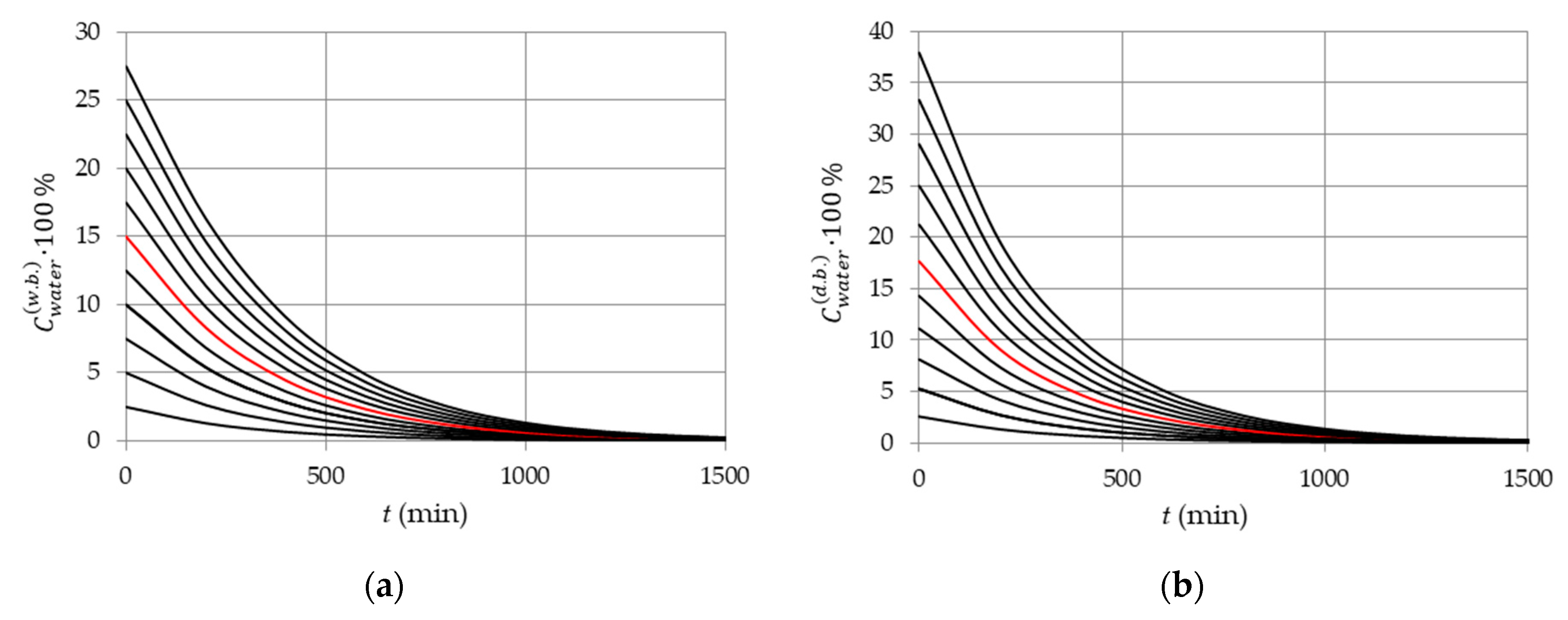
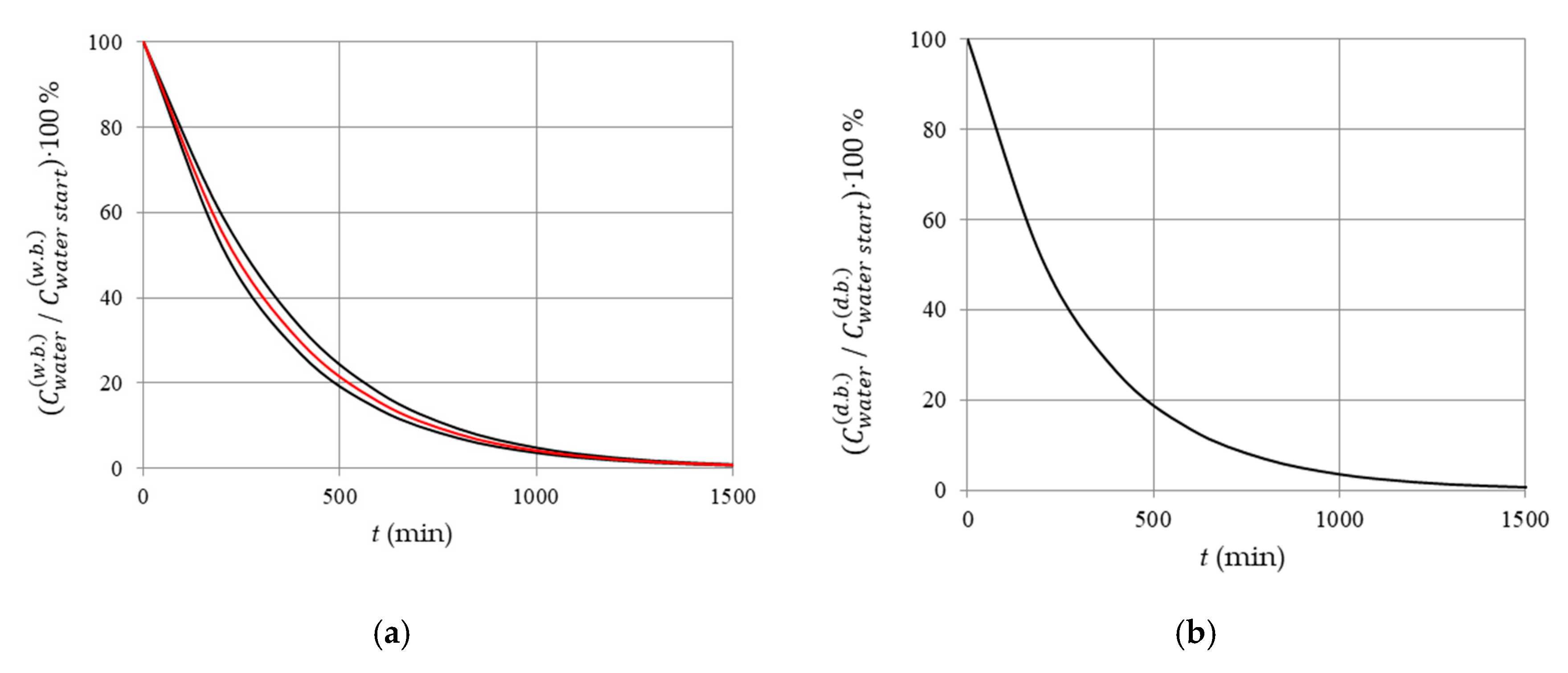
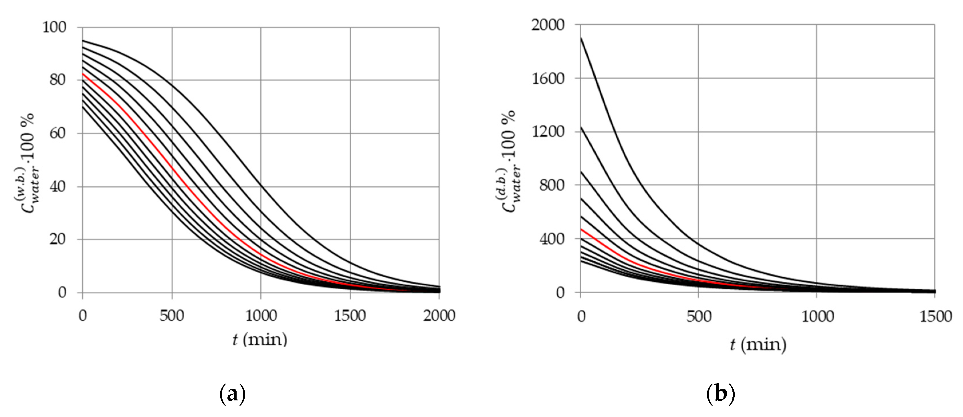
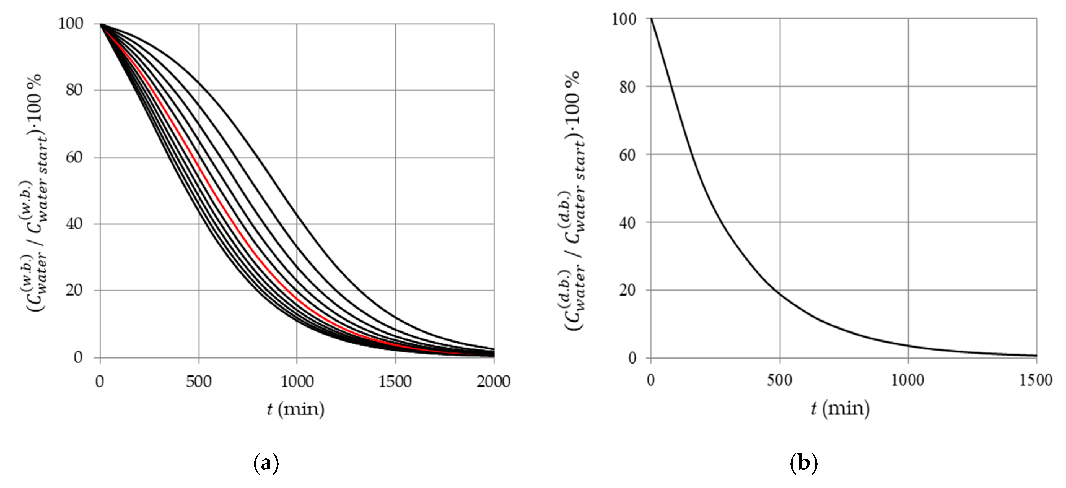
3.1. Influence of Initial Material Moisture Content (Wet Basis and Dry Basis)

Using the above relations (18), (18a), (20), and (21), we perform model calculations, the results of which illustrate the effect of the initial moisture content on the drying process. The simulation results are shown in Figure 2.

The following initial data were used in the calculations: initial moisture $C_{water,start}^{(w.b.)}$ = 0.025,…, 0.275 (Figure 2a); equivalent initial moisture content $C_{water,start}^{(d.b.)}$ = 0.026,…, 0.379, calculated by the Equation (8) (Figure 2b); parameter τ = 300 min (11) in all variants. Calculations are performed according to Equations (18a) (Figure 2a) and (21) (Figure 2b).

The normalized moisture content (Figure 3), depending on the basis (w.b. or d.b.), is defined as the ratio $C_{water}^{(w.b.)}/C_{water,start}^{(w.b.)}$ or $C_{water}^{(d.b.)}/C_{water,start}^{(d.b.)}$, respectively.

Figure 2 shows that if the initial moisture content is low enough (no more than 0.1), then the predicted moisture content is almost independent of the choice of the basis (w.b. or d.b.). However, with an increase in the initial moisture content, the influence of the choice of the basis also increases.

Figure 3b and Equation (22) show that the normalized initial moisture content (d.b.) in this model does not depend on the initial moisture content, in other words, the model may not be informative enough. At the same time, the normalized initial moisture content (w.b.) determined using Equation (18) reflects the influence of the initial moisture content:

$$\frac{C_{water}^{(w.b.)}}{C_{water,start}^{(w.b.)}}=\frac{1}{C_{water,start}^{(w.b.)}(1-e^{\theta })+e^{\theta }}$$

(22a)

Continuing the discussion, it is important to pay attention to Figure 1, from which it follows that the influence of the basis (w.b. or d.b.) will increase with increasing initial moisture content. This circumstance, as noted above, is not taken into account in the right-hand side of Equation (22), in contrast to Equation (22a). Therefore, the use of normalized moisture content (w.b.) (22a) may be more appropriate when simulating the drying of materials with high initial moisture content. To check this assumption, we perform calculations at a sufficiently high initial moisture content of the material (0.70, 0.725,…, 0.95 (w.b.), which is equivalent to the initial moisture interval (2.33,…, 19.00 (d.b.)). The simulation results are shown in Figure 4 and Figure 5. Calculations were performed using formulas (18a) (Figure 4a), (21) (Figure 4b), (22a) (Figure 5a), and (22) (Figure 5b).

Analysis of other features of the curves in Figure 4 and Figure 5 is performed in Section 3.2.

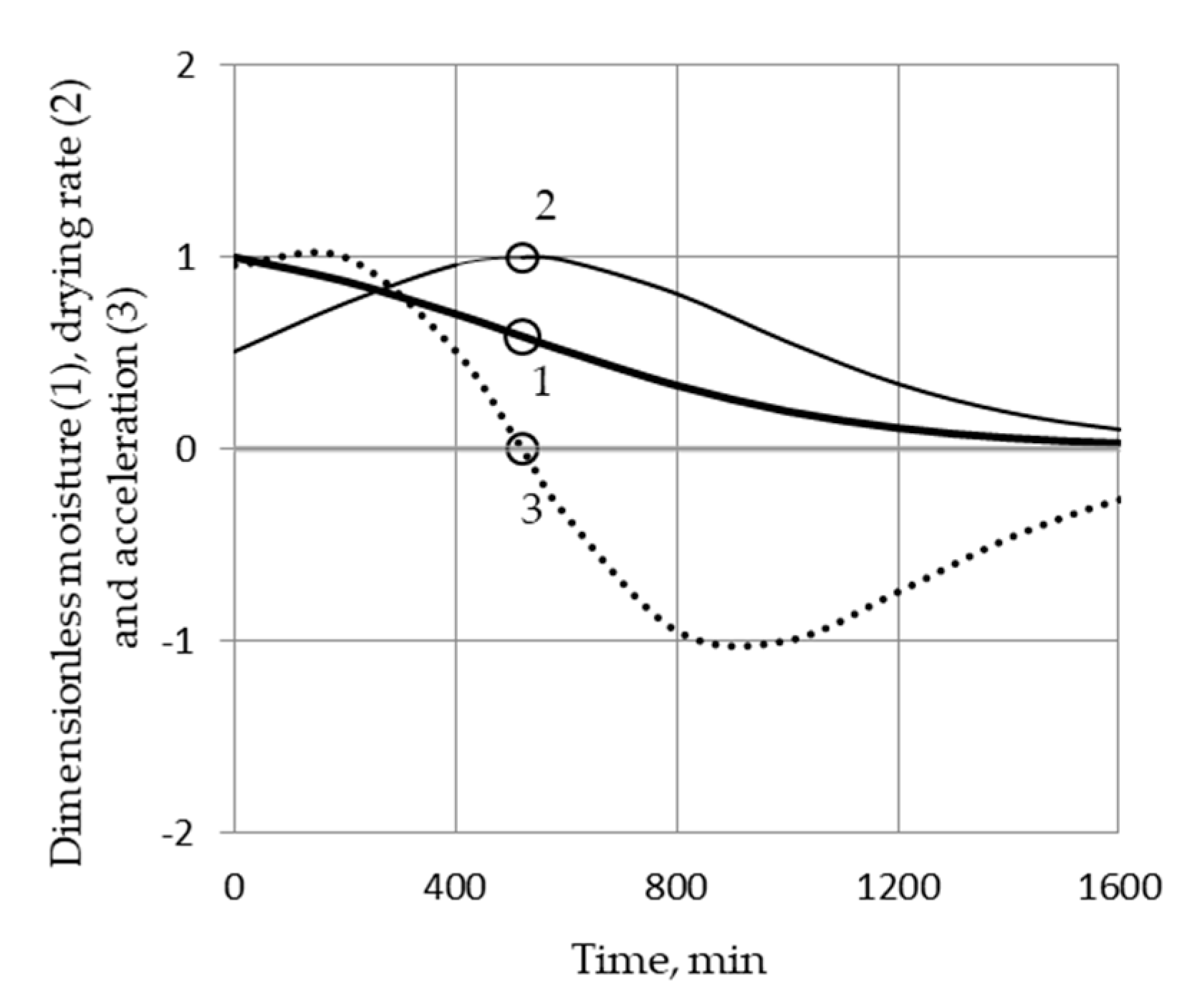
3.2. Inflection Point on the Drying Curve and the Rate of the Drying Process

Figure 4 and Figure 5 show that as the initial moisture content of the material increases, an inflection point appears on the curve in Figure 4a and Figure 5a, in contrast to the curve in Figure 4b and Figure 5b. Formally, this means that at the inflection point, the second derivative of the moisture function with respect to time is zero. Let t* be the abscissa of the inflection point; P—the right side of relation (22a). Then from the equation $\frac{d^{2}P}{d{t}^2}=0$, we find after transformations:

$$t^{*}=\tau \ln \frac{C_{water}^{(w.b.)}}{1-C_{water}^{(w.b.)}}$$

(22b)

In the problem under consideration t* ≥ 0, τ > 0. The physical meaning of the problem corresponds to such values $C_{water}^{(w.b.)}$, for which $\frac{C_{water}^{(w.b.)}}{1-C_{water}^{(w.b.)}}\ge 1$, i.e., 0.5 ≤ $C_{water}^{(w.b.)}$ < 1. For example, if $C_{water}^{(w.b.)}$ = 0.85 and τ = 300 min, then t* = 520.4 min.

The question then arises: What features of the drying process is simulated by the inflection point?

Answer: If an inflection point exists (22b), then the drying process rate increases up to the inflection point 0 < t < t*. At a point t = t*, the rate of the drying process reaches an extreme. If t > t*, then the rate of the drying process decreases. If T* = 0, then the drying rate only decreases from start to finish of this technological process.

Figure 6 illustrates the noted features of the drying process for material with high initial moisture content.

The initial moisture content $C_{water,start}^{(w.b.)}$ of the material and the parameter τ are equal to 0.85 and 300 min, respectively. Point 1 is the inflection point on the curve simulating the dependence of on time. At point 3, as noted above, $\frac{d^{2}P}{d{t}^2}=0, t=t^{*}$ 520.4 min. At point 2, the drying process rate is extreme at the same value of t.

Experimental data that confirm the existence of the above features of the drying process can be found in the literature, for example, in the graphs in Figure 2c from [20]. However, it was not possible to find a theoretical justification for these features, including analogs of relation (22b).

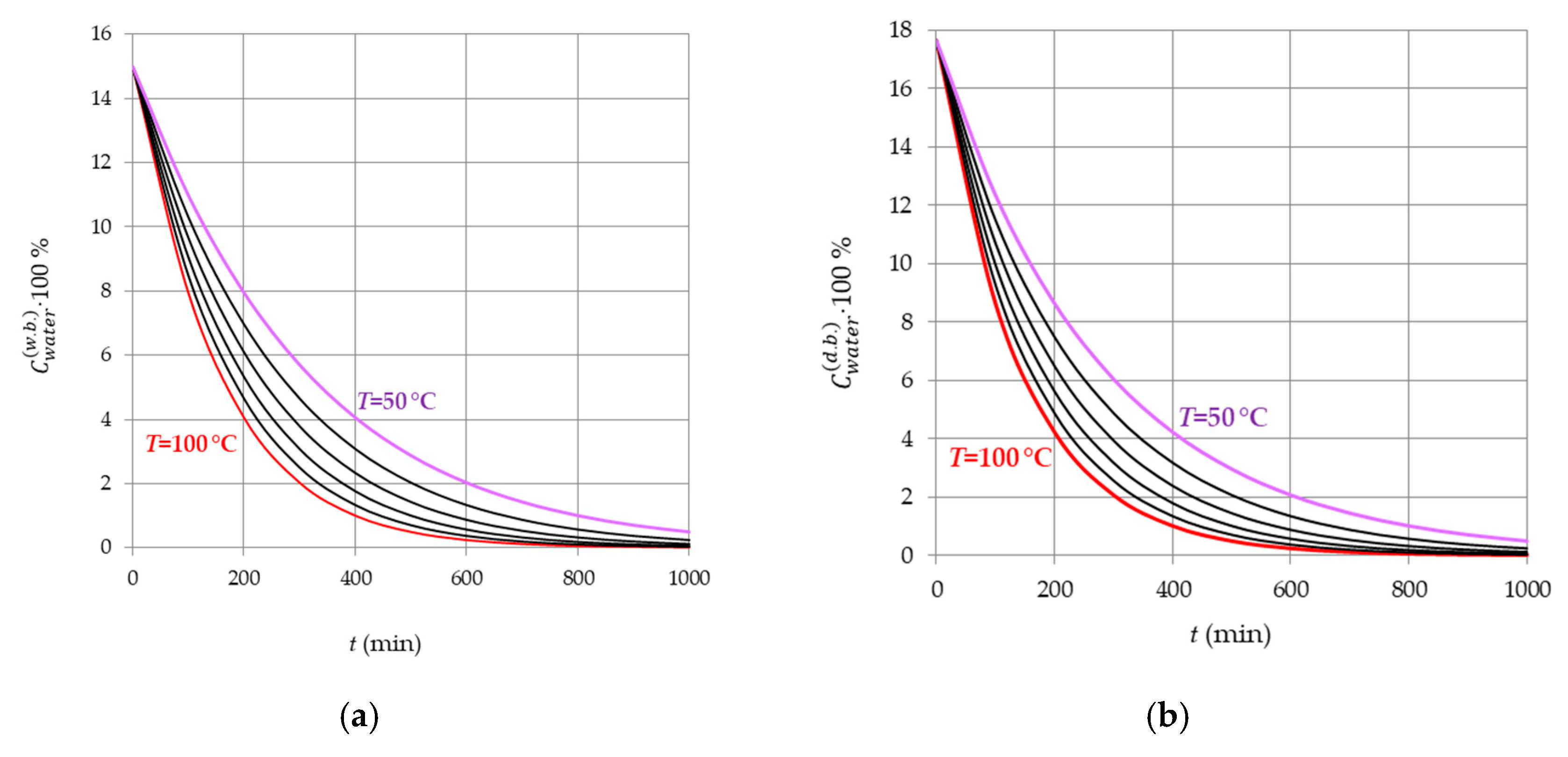
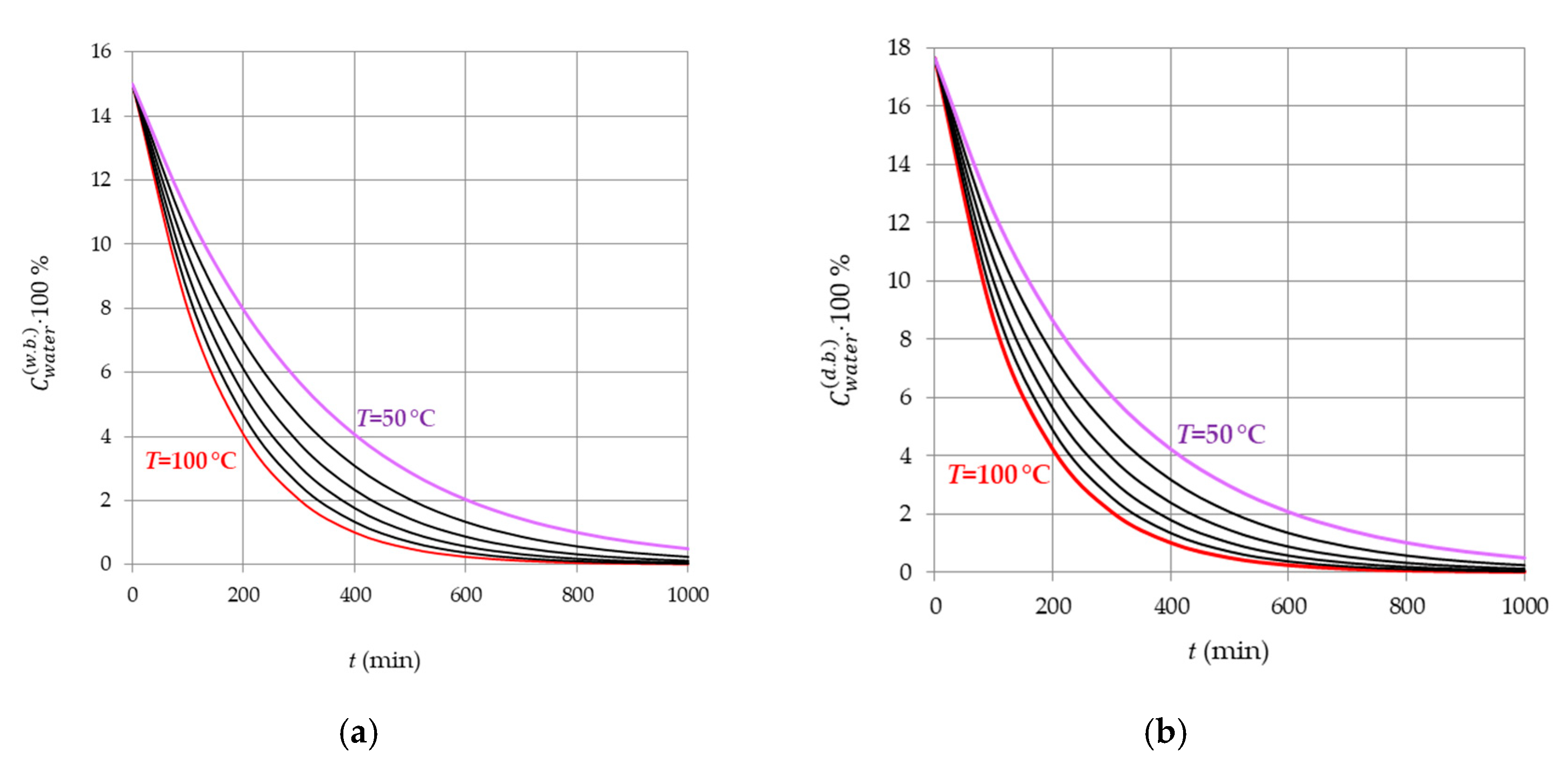
3.3. Influence of Drying Temperature

The dependence of moisture content on drying temperature can be taken into account indirectly, for example, by changing the coefficient k in Newton’s model. This issue was studied in more detail, for example, in [19], where, in particular, for modeling the drying of one of the materials at temperatures of 35, 45 and 55 °C, the values of coefficient k 0.34, 0.049 and 0.016, respectively, were obtained. A similar approach is used in [15]. Thus, the coefficient k summarizes the effect of temperature and other technological features of drying. Obviously, it is important for practice to know the influence of each factor on the drying process [1,22,23,24,25]. However, this is a difficult task. Let us consider a simple model in which the drying temperature and initial moisture content are separately taken into account; the influence of other factors is modeled in total.

Let’s use the results presented above to study one of the possible approaches to model building, taking into account the drying temperature in a thin layer.

Restricting ourselves to the option of drying at a positive temperature, we can assume that in relation (11), the value of ΔM_water is proportional to the amount of water M_water and the drying temperature T °C (in this work, the drying temperature is assumed to be a constant value; to take into account the temperature, a dimensionless coefficient ϕ = T °C/T_ref °C is used, where T_ref is the reference temperature equal to $100 °\mathrm{C}$. Thus, instead of (11), we can write:

$$\Delta M_{water}=\frac{\Delta t}{\tau }{M}_{water}\varphi$$

(23)

For substantiating relation (23), one can additionally refer to the work [26], (p. 11), according to which the change in the moisture content of the material is directly proportional to the temperature of the air for drying.

Regarding the coefficient ϕ, note that the value of T_ref = 100 °C is chosen to obtain the coefficient in dimensionless form. In the particular case under consideration, the choice of T_ref is not critical, i.e., another suitable value may be used, since possible deviations will be compensated by the above parameter τ. However, all temperature values in the considered model are assumed to be positive.

Using (23), following the logic of obtaining relations (14)–(18a), we write down relations (24)–(28):

$$\Delta M_{water}=\Delta \theta M_{water}\varphi$$

(24)

$${\tilde{C}}_{water}^{(w.b.)}=\frac{C_{water}^{(w.b.)}-\Delta \theta \varphi C_{water}^{(w.b.)}}{1-\Delta \theta \varphi C_{water}^{(w.b.)}}$$

(25)

$$\Delta C_{water}^{(w.b.)}=\Delta \theta \varphi C_{water}^{(w.b.)}\left(1-C_{water}^{(w.b.)}\right)$$

(26)

$$\frac{d{C}_{water}^{(w.b.)}}{C_{water}^{(w.b.)}(1-C_{water}^{(w.b.)})}=-d\varphi \theta$$

(27)

$$C_{water}^{(w.b.)}=\frac{C_{water,start}^{(w.b.)}}{C_{water,start}^{(w.b.)}(1-e^{\theta \varphi })+e^{\theta \varphi }}$$

(28)

By analogy with (18a), we transform (28) to the form (28a):

$$C_{water}^{(w.b.)}=\frac{e^{-\theta \varphi }}{{\left(C_{water,start}^{(w.b.)}\right)}^{-1}+e^{-\theta \varphi }-1}$$

(28a)

Using (28a), we find the moisture content $C_{water}^{(d.b.)}$ by using Equation (8).

By analogy with (22), let us determine the normalized values of moisture content in the form of ratios $C_{water}^{(w.b.)}/C_{water,start}^{(w.b.)}$, $C_{water}^{(d.b.)}/C_{water,start}^{(d.b.)}$.

Note that the models considered in this paper belong to the class of models of drying in a thin layer [1]. In models of drying a material in a thin layer, it is assumed that the temperature and moisture content of the material almost does not change over its thickness. If these changes are significant, then more complex models based on differential equations in partial derivatives are used [8,13,22,23,24,25] and numerical modeling [26,27]. To get an idea of the adequacy of model (28) from a physical point of view, it is necessary to compare it with experimental data.

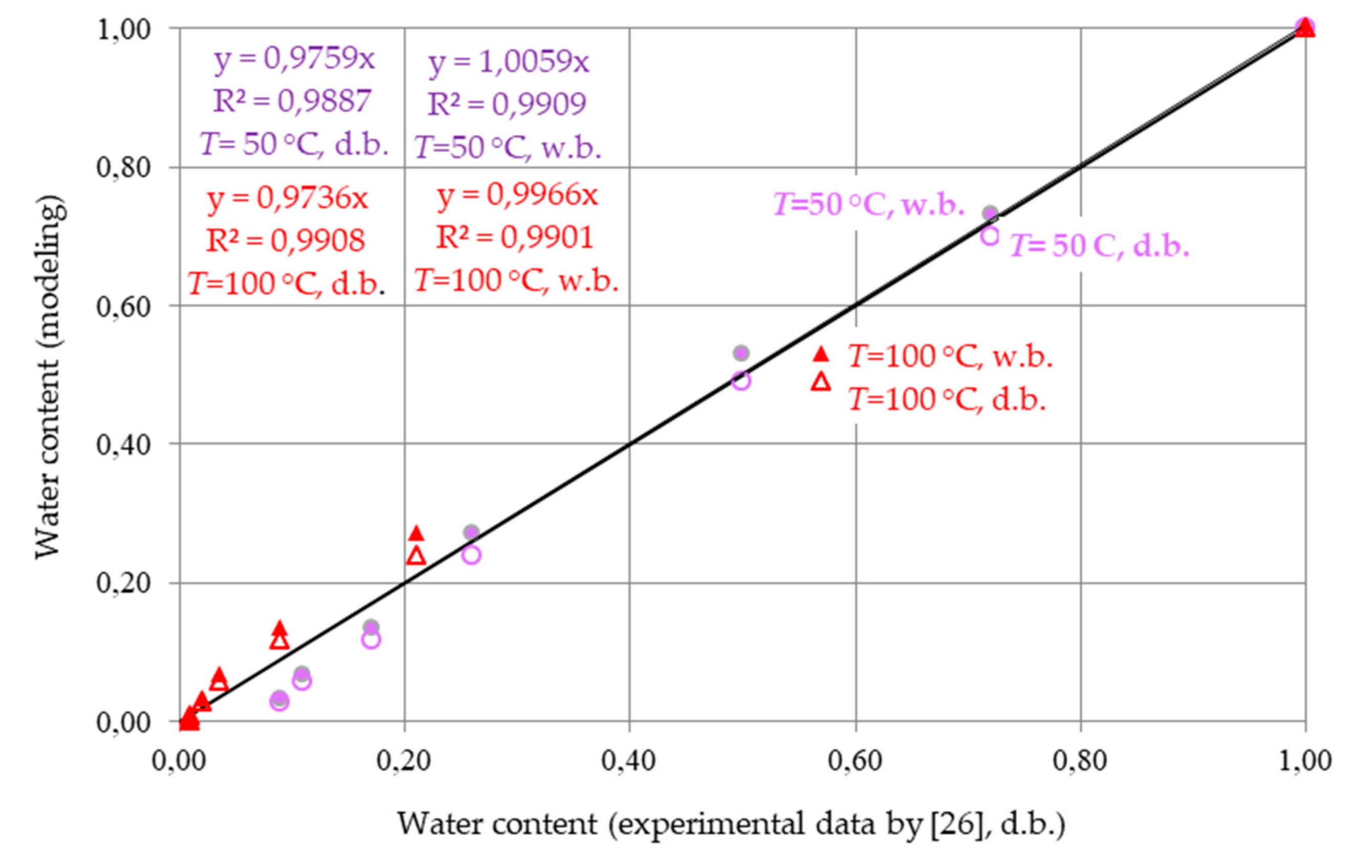
3.4. Comparison with the Experimental Data on Drying Ceramic Blocks for Construction, Known from the Literature

We will use the results of an experimental study of drying ceramic blocks for construction, known from the literature [26]. In this case, the use of models for drying a capillary-porous material in a thin layer is acceptable due to the fact that the thickness of the walls of the blocks is rather small (0.63,…, 0.94 cm) [26,27].

The initial moisture content of the material is ~0.17 (d.b.) (Table 1 in [26]), which according to (7) corresponds to $C_{water}^{(w.b.)}$ = 0.17/(1 + 0.17) ≈ 0.15. In the cited work [26], experimental data on the change in the moisture content of the same material over time are given in graphical form for a number of experiments in which the drying temperature was 50, 60, 70, 80, 90, and 100 °C. The simulation results obtained using relations (24)–(28a) are shown in Figure 7 and Figure 8. $\tau =140\min$ (see Section 3.4). The consistency of the experimental and calculated data is illustrated in Figure 9.

Due to the fact that the data presented in Figure 8 confirm the adequacy of the model and the reliability of the simulation results. The characteristic of the process rate can be the slope ratio of the tangent to the curves in Figure 7 and Figure 8. If the drying temperature increases, then the rate of this process also increases, and the time to completion of the process decreases, which corresponds to the data known from the literature.

Figure 7 and calculations by Equation (28a) show that when drying to a moisture content of 0.04 (w.b.) at a temperature of 50, 60,…, 100 °C, each successive temperature step (10 °C) corresponds to decreasing time intervals. This feature can be explained by the fact that the relative value of the temperature increment decreases with each step. In other words, an increase in temperature from 50 to 60 °C means an increase in temperature by 10/50 = 20%; from 60 to 70 °C—by 10/60 ≈ 17%; from 90 to 100 °C—by 10/90 ≈ 11%. These results do not contradict the experimental studies known from the literature [26], according to which the rate of change in the moisture content of the material is directly proportional to the drying temperature.

3.5. Analysis of the Results: Methodological Aspects

The results presented above allow us to answer a question that is important from a practical point of view: what is the physical meaning of the coefficient τ in Equations (11), (12), (22), etc.? Also, it is methodologically important to know how to calculate the coefficient τ? To search for answers, we will use relations (22).

Let’s write: $C_{water}^{(d.b.)}\left(t\right)=C_{water.,start}^{(d.b.)}{e}^{\frac{t}{\tau }}$. Let τ = t. Then $C_{water}^{(d.b.)}=C_{water,start}^{(d.b.)}{e}^{-1}$ ≈ $C_{water,start}^{(d.b.)}/2.718$ Consequently, the value τ is equal to the drying time t at which the moisture content decreases by a factor e ≈ 2.718.

To calculate the coefficient τ, it is necessary to carry out a test drying and build a plot of the dependence $C_{water}^{(d.b.)}\left(t\right)$. The point on the plot for which $C_{water}^{(d.b.)}\approx C_{water,start}^{(d.b.)}/2.718$ corresponds to t = τ.

If we use formula (28a), then the coefficient τ is calculated in the same way, but in this case the test drying is carried out only at a temperature of T = T_ref, i.e., for ϕ = 1 in Equation (23). This is how the value τ = 140 min was found for the above modeling results (Figure 7 and Figure 8).

The presented method for determining coefficient $\tau$ is recommended for calculations on wet and dry basis. The transition from one basis to another is carried out according to Equation (7).

With regard to calculations on a wet and dry basis, it is methodologically important to note the following. Figure 2 and Figure 3 show that calculations results on a wet and dry basis are practically equivalent at low moisture. However, as moisture increases, the equivalence of the calculated data on a wet and dry basis is lost (Figure 4 and Figure 5). Taking this circumstance into account, it is possible to formulate restrictions on the field of application of the calculation formulas, for which, however, further experimental and theoretical studies are required. From a methodological point of view, it is important to note that in this work a phenomenological approach was used to modeling changes in the moisture content of a capillary-porous material in a thin layer. This approach is used in applied sciences, for example, [28,29]. As is known, phenomenological models take into account only the observed (external) properties of objects and do not take into account the internal mechanisms of phenomena, for example, the change in the moisture content of a capillary-porous material is studied without detailed analysis of moisture transfer. A detailed consideration of the transfer of mass and heat would lead to a model that belongs to a different class [8,25]. Analysis of models that do not belong to the class of phenomenological models is beyond the scope of our work.

4. Conclusions

(1)

A mathematical model has been developed for thin-layer drying of a capillary-porous material with direct consideration of its initial moisture content and drying temperature, along with indirect consideration of the influence of other factors.

(2)

Using the developed model, the analysis of the features of the drying process of materials with high and low initial moisture content has been carried out. The dependence of the ratios of the normalized moisture content on the choice of the basis (w.b. or d.b.) has been proved.

(3)

It is shown that the function of normalized moisture content (w.b.) directly depends on the initial moisture content and, as a consequence, is more informative than the function of normalized moisture content (d.b.), in which the initial moisture content is indirectly and indiscernibly taken into account in combination with the temperature and other technological factors of drying. It was found that if the initial moisture content (w.b.) is in the range (0.5; 1.0), then the rate of the drying process reaches an extreme in this range. An analytical relationship for determining the time at which the drying rate is extreme has been substantiated.

(4)

The developed mathematical model of thin-layer drying makes it possible to predict changes in the moisture content of the material and the duration of its drying, depending on the initial moisture content of the material and the drying temperature. Thus, the number of indirectly taken into account factors has been reduced, which, accordingly, increases the predictive capabilities of the model when justifying recommendations for improving drying technologies in the interests of sustainable development.

(5)

The adequacy of the model and the assessment of the reliability of the results of model calculations are confirmed by their agreement with the experimental data related to the drying of ceramic blocks for construction, known from the literature.

References

1. Kucuk, H.; Midilli, A.; Kilic, A.; Dincer, I. A Review on Thin-Layer Drying-Curve Equations. Dry. Technol. 2014, 32, 757–773. [Google Scholar] [CrossRef]
2. Jayas, D.S.; Cenkowski, S.; Pabis, S.; Muir, W.E. Review of thin-layer drying and wetting equations. Dry. Technol. 1991, 9, 551–588. [Google Scholar] [CrossRef]
3. Ostanek, J.; Ileleji, K. Conjugate heat and mass transfer model for predicting thin-layer drying uniformity in a compact, crossflow dehydrator. Dry. Technol. 2020, 38, 775–792. [Google Scholar] [CrossRef]
4. Visser, R.; Berkett, H.; Spinelli, R. Determining the effect of storage conditions on the natural drying of radiata pine logs for energy use. N. Z. J. Sci. 2014, 44. [Google Scholar] [CrossRef] [Green Version]
5. Asdrubali, F.; Ferracuti, B.; Lombardi, L.; Guattari, C.; Evangelisti, L.; Grazieschi, G. A review of structural, thermo-physical, acoustical, and environmental properties of wooden materials for building applications. Build. Environ. 2017, 114, 307–332. [Google Scholar] [CrossRef]
6. Sadłowska-Sałęga, A.; Wąs, K. Risk of Moisture in Diffusionally Open Roofs with Cross-Laminated Timber for Northern Coastal Climates. Buildings 2020, 10, 10. [Google Scholar] [CrossRef] [Green Version]
7. Teaca, C.A.; Roşu, D.; Mustaţă, F.; Rusu, T.; Roşu, L.; Roşca, I.; Varganici, C.D. Natural Bio-Based Products for Wood Coating and Protection against Degradation: A Review. Bio. Resour. 2019, 14, 4873–4901. [Google Scholar] [CrossRef]
8. Pecenko, R.; Challamel, N.; Colinart, T.; Picandet, V. Semi-analytical solution of Luikov equations for time-periodic boundary conditions. Int. J. Heat Mass. Transfer. 2018, 124, 533–542. [Google Scholar] [CrossRef]
9. Silva, W.P.; Silva, C.M.D.P.S.; Silva, L.D.; Farias, V.S.O. Drying of clay slabs: Experimental determination and prediction by two-dimensional diffusion models. Ceram. Int. 2013, 39, 7911–7919. [Google Scholar] [CrossRef]
10. Mitterpach, J.; Igaz, R.; Štefko, J. Environmental evaluation of alternative wood-based external wall assembly. Acta Fac. Xylol. Zvolen Res. Publica Slovaca 2020, 62, 133–149. [Google Scholar] [CrossRef]
11. Huang, S.; He, Q.; Miao, Z.; Wan, K.; Wan, Y. Multiphysics modeling of water transport in high-intensity lignite drying process on pore scale. Energy Sources Part A Recovery Util. Environ. Effects 2018, 40, 2580–2589. [Google Scholar] [CrossRef]
12. Golisz, E.; Jaros, M.; Głowacki, S. Modelling of biomass temperature in the drying process. E3S Web Conf. 2020, 154, 1004. [Google Scholar] [CrossRef] [Green Version]
13. Defraeye, T. Advanced Computational Modelling for Drying Processes—A Review. Appl. Energy 2014, 131, 323–344. [Google Scholar] [CrossRef]
14. Agbossou, K.; Napo, K.; Chakraverty, S. Mathematical Modelling and Solar Tunnel Drying Characteristics of Yellow Maize. Am. J. Food Sci. Technol. 2016, 4, 115–124. [Google Scholar] [CrossRef]
15. Cuevas, M.; Martínez-Cartas, M.L.; Pérez-Villarejo, L.; Hernández, L.; García-Martín, J.F.; Sánchez, S. Drying kinetics and effective water diffusivities in olive stone and olive-tree pruning. Renew. Energy 2019, 132, 911–920. [Google Scholar] [CrossRef]
16. Soodmand-Moghaddam, S.; Sharifi, M.; Zareiforoush, H.; Mobli, H. Mathematical modeling of lemon verbena leaves drying in a continuous flow dryer equipped with a solar pre-heating system. Qual. Assur. Saf. Crop. Foods 2020, 12, 57–66. [Google Scholar] [CrossRef]
17. Górnicki, K.; Kaleta, A.; Choińska, A. Suitable model for thin-layer drying of root vegetables and onion. Int. Agrophys. 2020, 1, 79–86. [Google Scholar] [CrossRef]
18. Kantyshev, A.V.; Zaitseva, M.I.; Kolesnikov, G.N. Model of wood impregnation after incomplete drying as an additional energy management tool. J. Phys. Conf. Ser. 2019, 1333, 032033. [Google Scholar] [CrossRef]
19. Ivanova, M.; Katrandzhiev, N.; Dospatliev, L. Using some mathematical models in modeling mushroom drying (agaricus bisporus). Int. J. Appl. Math. 2020, 33, 109–124. [Google Scholar] [CrossRef]
20. Nigay, N.A.; Kuznetsov, G.V.; Syrodoy, S.V.; Gutareva, N.Y. Estimation of energy consumption for drying of forest combustible materials during their preparation for incineration in the furnaces of steam and hot water boilers. Energy Sources Part A Recovery Util. Environ. Effects 2020, 42, 1997–2005. [Google Scholar] [CrossRef]
21. Oosawa, K.; Kanematsu, Y.; Kikuchi, Y. Forestry and Wood Industry. In Energy Technology Roadmaps of Japan; Kato, Y., Koyama, M., Fukushima, Y., Nakagaki, T., Eds.; Springer: Tokyo, Japan, 2016. [Google Scholar] [CrossRef]
22. Dong, W.; Chen, Y.; Bao, Y.; Fang, A. A validation of dynamic hygrothermal model with coupled heat and moisture transfer in porous building materials and envelopes. J. Build. Eng. 2020, 101484. [Google Scholar] [CrossRef]
23. Caccavale, P.; De Bonis, M.V.; Ruocco, G. Conjugate Heat and Mass Transfer in Drying: A Modeling Review. J. Food Eng. 2016, 176, 28–35. [Google Scholar] [CrossRef]
24. Koukouch, A.; Bakhattar, I.; Asbik, M.; Idlimam, A.; Zeghmati, B.; Aharoune, A. Analytical solution of coupled heat and mass transfer equations during convective drying of biomass: Experimental validation. Heat Mass Transf. 2020, 56, 1971–1983. [Google Scholar] [CrossRef]
25. Luikov, A.V. Systems of differential equations of heat and mass transfer in capillary-porous bodies. Int. J. Heat Mass Transf. 1975, 18, 1–14. [Google Scholar] [CrossRef]
26. Da Silva, A.M.V.; Delgado, J.M.P.Q.; Guimarães, A.S.; de Lima, W.M.P.B.; Gomez, R.S.; de Farias, R.P.; de Lima, E.S.; de Lima, A.G.B. Industrial Ceramic Blocks for Buildings: Clay Characterization and Drying Experimental Study. Energies 2020, 13, 2834. [Google Scholar] [CrossRef]
27. De Vasconcellos, M.A.; de Brito Correia, B.R.; Brandão, V.A.A.; de Oliveira, I.R.; Santos, R.S.; de Oliveira Neto, G.L.; de Lucena Silva, L.P.; de Lima, A.G.B. Convective Drying of Ceramic Bricks by CFD: Transport Phenomena and Process Parameters Analysis. Energies 2020, 13, 2073. [Google Scholar] [CrossRef] [Green Version]
28. Merlin, O.; Olivera-Guerra, L.; Hssaine, B.A.; Amazirh, A.; Rafi, Z.; Ezzahar, J.; Gentinec, P.; Khabbab, S.; Gascoina, S.; Er-Raki, S. A phenomenological model of soil evaporative efficiency using surface soil moisture and temperature data. Agric. For. Meteorol. 2018, 256, 501–515. [Google Scholar] [CrossRef] [Green Version]
29. Bisson, A.; Rigacci, A.; Lecomte, D.; Rodier, E.; Achard, P. Drying of silica gels to obtain aerogels: Phenomenology and basic techniques. Dry. Technol. 2003, 21, 593–628. [Google Scholar] [CrossRef]
Figure 1. The relationship between moisture values determined on the wet basis and on the dry basis.
Applsci 10 06953 g001
Figure 2. Change in moisture content (w.b. (a) and d.b. (b)) depending on time at the initial moisture content C w a t e r , s t a r t ( w . b . ) = 0.025, 0.05,…, 0.15,…, 0.275.
Applsci 10 06953 g002
Figure 3. Normalized moisture content (w.b. (a) and d.b. (b)) depending on time at the initial moisture content by Figure 2. Ratio C w a t e r ( d . b . ) / C w a t e r , s t a r t ( d . b . ) is indifferent to initial moisture.
Applsci 10 06953 g003
Figure 4. Change in moisture content (w.b. (a) and d.b. (b)) depending on time at the initial moisture content 0.70, 0.725,…, 0.825, …, 0.95 (w.b.).
Applsci 10 06953 g004
Figure 5. Normalized moisture content (w.b. (a) and d.b. (b)) depending on time at the initial moisture content (w.b.) by Figure 4. The ratio C w a t e r ( d . b . ) / C w a t e r , s t a r t ( d . b . ) is independent of the initial moisture content (22).
Applsci 10 06953 g005
Figure 6. Normalized dimensionless characteristics: moisture content (w.b.), drying rate module and drying process acceleration.
Applsci 10 06953 g006
Figure 7. Dependence of moisture content (w.b. (a) and d.b. (b)) on time and drying temperature 50, 60,…, 100 °C at the initial material moisture of 0.15 (w.b.).
Applsci 10 06953 g007
Figure 8. Normalized moisture content (w.b. (a) and d.b. (b)) depending on the time and drying temperature 50, 60,…, 100 °C at the initial material moisture of 0.15 (w.b.).
Applsci 10 06953 g008
Figure 9. Comparison of experimental and calculated values of normalized moisture content (w.b. and d.b.). Drying temperature: 50 and 100 °C. Initial material moisture: 0.15 (w.b.) 0.17 (d.b.). The experimental data were obtained after processing the plots according to Figure 8 in paper [26].
Applsci 10 06953 g009