Estimation of Distribution Algorithms with Fuzzy Sampling for Stochastic Programming Problems

Abstract

Generating practical methods for simulation-based optimization has attracted a great deal of attention recently. In this paper, the estimation of distribution algorithms are used to solve nonlinear continuous optimization problems that contain noise. One common approach to dealing with these problems is to combine sampling methods with optimal search methods. Sampling techniques have a serious problem when the sample size is small, so estimating the objective function values with noise is not accurate in this case. In this research, a new sampling technique is proposed based on fuzzy logic to deal with small sample sizes. Then, simulation-based optimization methods are designed by combining the estimation of distribution algorithms with the proposed sampling technique and other sampling techniques to solve the stochastic programming problems. Moreover, additive versions of the proposed methods are developed to optimize functions without noise in order to evaluate different efficiency levels of the proposed methods. In order to test the performance of the proposed methods, different numerical experiments were carried out using several benchmark test functions. Finally, three real-world applications are considered to assess the performance of the proposed methods.

1. Introduction

Several real-world applications can be formulated as continuous optimization problems in a wide range of scientific domains, such as engineering design, medical treatment, supply chain management, finance, and manufacturing [1,2,3,4,5,6,7,8,9]. Many of these optimization formulations have some sort of uncertainty and their objective functions contain noise [10,11,12,13]. Moreover, it is sometimes necessary to deal with complex problems with high nonlinearity and/or dimensionality, and occasionally there is no analytical form for the objective function [14]. Even if the objective functions associated with these types of problems are expressed mathematically, in most cases they are not differentiable. Therefore, classical optimization methods fail to adapt them, and it is impossible to compute their gradient. The situation is much worse when these functions contain high noise levels.

Simulation and optimization has attracted much interest recently, since the output response evaluation of such real-world problems need simulation techniques. Moreover, optimization problems in stochastic environments are realized by combining simulation-based estimation with an optimization process. Therefore, the title “simulation-based optimization” is commonly used instead of “stochastic optimization” [15,16].

Simulation-based optimization is used with certain types of uncertainties to optimize the real-world problem. There are four types of uncertainties discussed in [14]: noise in objective function evaluations; approximation of computationally expensive objective functions with surrogate models; changes or disturbance of design parameters after determining the optimal solution; problems with time-varying objective functions. We consider the first type of uncertainty, where the problem is defined mathematically as follows [17]:

$$\underset{x\in X}{min}\{f\left(x\right)=\mathbb{E}\left[\mathfrak{F}(x,\omega )\right]\},$$

(1)

where f is a real-valued function defined on search space $X\subseteq R^n$ with objective variables $x\in X$, and $\omega$ is a random variable whose probability density function is $\mathfrak{F}$. Problem (1) is also referred to as the stochastic programming problem in which random variables appear in the formulation of the objective functions.

In spite of the importance of the choice of optimal simulation parameters in improving operation, configuring them well still remains a challenge. Because of the complicated simulation process, the objective function is subjected to different noise levels followed by expensive computational evaluation. These problems are restricted by the following characterizations:

• The complexity and time necessary to compute the objective function values;
• The difficulty of computing the exact gradient of the objective function, as well as its numerical approximation being very expensive;
• The noise values in the objective function.

To deal with these characterizations, global search methods should be invoked to avoid using classical nonlinear programming that fails to solve such problems with multiple local optima.

Recently, the use of artificial intelligence methods in optimization has been of great interest. Metaheuristics play a significant role in both real-life simulations and invoking smart methods [18,19,20,21,22,23,24]. Metaheuristics show strong validity rates across a wide variety of applications. These methods, however, suffer from slow convergence, especially in cases of complex applications, which lead to high computational costs. This slow convergence may be a result of the exploration structures of such methods, while exploring the search space depends on the random structures. On another hand, metaheuristics cannot utilize local information to deduce promising search directions. The estimation of Distribution Algorithms (EDAs) comprise a class of evolutionary computation [25] and has been widely studied in the global optimization field [26,27,28,29]. Compared with traditional Evolutionary Algorithms (EAs), such as Genetic Algorithms (GAs), this type of algorithm has neither crossover nor mutation operators. Instead, an EDA explicitly builds a probabilistic model by learning and sampling the probability distribution of promising solutions in each generation. While building the probabilistic model presents statistical information from the search space, it is used as the guidance of reproduction to find better solutions.

On the other hand, several optimal search techniques have been designed to tackle the stochastic programming problem. Some of these techniques are known as variable-sample methods [30]. The key aspect of the variable-sample approach is to reformulate the stochastic optimization problem in the form of a deterministic one. A differential evolution variant is proposed in [12] equipped with three new algorithmic components, including a central tendency-based mutation, adopted blending crossover, and a new distance-based selection mechanism. To deal with the noise, their algorithm uses non-conventional mutation strategies. In [31], an extension of multi-objective optimization is proposed, based on an differential evolution algorithm to manage the effect of noise in objective functions. Their method applies an adaptive range of the sample size for estimating the fitness values. In [32], instead of using averages, the search policy considers the distribution of noisy samples during the fitness evaluation process. A number of different approaches to deal with noise are presented in [33]. Most sampling methods are based on the use of averages, and this motivates us to use different sampling techniques. One possible sampling alternative is the use of fuzzy logic, which is an important pillar of computational intelligence. The idea of the fuzzy set was first introduced in [34]; this enabled a member to belong to a set in a partitioned way, as opposed to in a definite way, as stated by classical set theory. In other words, membership can be assigned a value within the $[0,1]$ interval instead of the $\{0,1\}$ set. Over the past four decades, the theory of fuzzy random variables [35] has been developed via a large number of studies in the area of fuzzy stochastic optimization [36,37]. The noisy part of our problem can be considered to be randomness or fuzziness, and it can be understood as a fuzzy stochastic problem, which can be found in the literature [38,39,40,41,42].

In this paper, EDAs are used to solve nonlinear optimization problems that contain noise. The proposed EDA-based methods follow the class of EDAs proposed in [43]. The designed EDA-model is firstly combined with variable-sample methods (SPRS) [30]. Sampling techniques have a serious problem when the sample size is small, so estimating the objective function values with noise is accurate in these cases. Therefore, we propose a new sampling technique based on fuzzy systems to deal with small sample sizes. Another EDA-based method uses the proposed fuzzy sampling technique. Moreover, additive versions of the proposed methods are developed to optimize functions without noise in order to evaluate different efficiency levels of the proposed methods. In order to test the performance of the proposed methods, different numerical experiments were carried out using several benchmark test functions. Moreover, three real-world applications are considered to assess the performance of the proposed methods.

The rest of the paper is structured as follows. In Section 2, we highlight the main structure and techniques for EDAs. The design elements and proposed methods are stated in Section 3. In Section 4, algorithmic implementations of the proposed methods and numerical experiments are discussed. The results for three stochastic programming applications are presented in Section 5. Finally, the paper is concluded in Section 6.

2. Estimation of Distribution Algorithms

EDAs were firstly introduced in [44] as a new population-based method, and have been extensively studied in the field of global optimization [26,44]. Despite the fact that EDAs were firstly proposed for combinatorial optimization, many studies have been performed applying them to continuous optimization. The primary difference between EDAs is the aspect of building the probabilistic model. Generally, in continuous optimization there are two considerable branches: one is based on the Gaussian distribution model [25,26,45,46,47,48,49,50,51], and the other on the histogram model [47,52,53,54,55,56,57,58]. The first is the most widely used and has been studied extensively. The main steps of general EDAs are stated in Algorithm 1.

Algorithm 1 Pseudo-code for EDA approach

1: $g\leftarrow 0$

2 $P_g\leftarrow$ Generate and evaluate M random individuals (the initial population).

3: repeat

4: $P_g^s\leftarrow$ Select $m(\le M)$ individuals from $P_g$ according to a selection method.

5: $D_g\left(x\right)=p_g\left(x\right|P_g^s)\leftarrow$ Estimate the joint probability distribution of the selected individuals.

6: $P_{g+1}\leftarrow$ Generate M individuals using $D_g\left(x\right)$, and evaluate them.

7: $g\leftarrow g+1.$

8: until a stopping criterion is met.

In the case of adapting a Gaussian distribution model $D_g\left(x\right)$ in Algorithm 1, it has the form of a normal density with a mean $\widehat{\mu }$ and a covariance matrix $\mathsf{\Sigma }$. The earliest proposed EDAs were based on simple univariate Gaussian distributions, such as the Marginal Distribution Algorithm for continuous domains ($UMD{A}_c^G$) and Population-Based Incremental Learning for continuous domains ($PBI{L}_c$) [26,45]. In these, all variables are taken to be completely independent of each other, and the joint density function is

$$f_{\mathit{l}}(\mathbf{x};{\mathsf{\Theta }}^{\mathit{l}})=\prod _{i=1}^n{f}_{\mathit{l}}({\mathbf{x}}_{\mathbf{i}};{\mathsf{\Theta }}_{\mathbf{i}}^{\mathit{l}}),$$

(2)

where ${\mathsf{\Theta }}^{\mathit{l}}$ is a set of local parameters. Such models are simple and easy to implement with a low computational cost, but they fail with high dependent variable problems. For this problem, many EDAs based on multivariate Gaussian models have been proposed, which adapt the conventional maximum likelihood-estimated multivariate Gaussian distribution, such as Normal IDEA [46,47], EMNA${}_{global}$ [26], and EGNA [25,26]. These methods have the same performance, since they are based on the same multivariate Gaussian distribution, and there is no significant difference between them [26]. However, in these methods the dependence between variables is taken, so they have a poor exploitative ability and the computational cost increases exponentially with the problem size [59]. To address this problem, various extensions of these methods have been introduced, which depend on scaling $\mathsf{\Sigma }$ after estimating the maximum likelihood according to certain criteria to improve the exploration quality. This has been done in methods such as EEDA [48], SDR-AVS-IDEA [50], and CT-AVS-IDEA [49].

The EDA with Model Complexity Control (EDA-MCC) method was introduced to control the high complexity of the multivariate Gaussian model without losing the dependence between variables [43]. Since the univariate Gaussian model has a simple structure and limited computational cost, it has difficulty solving nonseparable problems. On other hand, the multivariate Gaussian model can solve nonseparable problems, but it usually has difficulty as a result of its complexity and cost. In the EDA-MCC method, the advantages of the univariate and multivariate Gaussian models are combined according to certain criterion and by applying two main strategies:

• Weakly Dependent Variable Identification (WI). In this strategy, the correlation coefficients between variables are calculated to measure how much they are dependent. This means that the observed linear dependencies are measured by their correlation coefficient with each other, as follows:

  $$corr(x_i,x_j)=\frac{cov(x_i,x_j)}{{\sigma }_i{\sigma }_j},$$

  (3)

  where $corr(x_i,x_j)$ is the linear correlation coefficient between $x_i$ and $x_j$, $cov(x_i,x_j)$ is their covariance, ${\sigma }_i$ and ${\sigma }_j$ are their standard deviations, respectively, and $i,j=1,\cdots ,n.$ Briefly, all variables are divided into two sets: W and S, where W is the set of weakly dependence variables, and S is the set of strong dependent variables. These variable sets are defined as follows:

  $$\begin{array}{ccc}\hfill W& =& \{x_i:|corr(x_i,x_j)|\le \theta ,\forall j=1,\dots ,n,j\ne i,i=1,\dots ,n\},\hfill \end{array}$$

  (4)

  $$\begin{array}{ccc}\hfill S& =& \{x_i:x_i\notin W,i=1,\dots ,n\},\hfill \end{array}$$

  (5)

  where $\theta$ is a threshold $(0\le \theta \le 1)$, and this reflects how much the user trusts the univariate model in the problem. Algorithm 2 shows the main flow of the WI strategy.

  Algorithm 2 Pseudo-code for WI

  1: Use m individuals to calculate the correlation matrix $C=\left(c_{ij}\right),$ where $c_{ij}=corr(x_i,x_j),i,j=1,\dots ,n.$

  2: Use C to construct W and S as defined in Equations (4) and (5), respectively.

  3: Estimate a univariate model for W based on the m selected individuals.

• Subspace Modeling (SM). This strategy is applied on the S set. The performance of the multivariate model needs a large population size and the complexity of computations increases frequently. The SM strategy is applied on the variables set in S, which preferably has a limited number of variables. If the size $\left|S\right|$ of set S is not limited, then the population points are projected to several subspaces of the n dimensional search space. Then, a multivariate model can be built for each subspace, which means that the dependence is considered only between variables in the same subspace. The main steps of the SM strategy are explained in Algorithm 3.

  Algorithm 3 Pseudo-code for SM

  1: Construct S as in Equation (5).

  2: Randomly partition S into $\lceil \left|S\right|/c\rceil$ nonintersected subsets: $S_1,S_2,\dots S_{\lceil \left|S\right|/c\rceil }$.

  3: Estimate a multivariate model for each subset based on m selected individuals.

  Parameter c is a predefined one that controls the number of the subspaces, where $(1\le c\le n)$.
  After carrying out the WI and SM strategies, the final joint probability distribution function (pdf) has the following form:

  $$f\left({\mathbf{x}}_i\right)=\prod _{x_i\in W}{\varphi }_i\left({\mathbf{x}}_{\mathbf{i}}\right)·\prod _{k=1}^{\lceil \left|S\right|/c\rceil }{\psi }_k\left({\mathbf{s}}_{\mathbf{k}}\right),$$

  (6)

  where ${\varphi }_i(·)$ is the univariate pdf of variable $x_i\in W$, and ${\psi }_k(·)$ is the multivariate pdf of the variables in $S_k$. The main steps of the EDA-MCC method are illustrated in Algorithm 4.

  Algorithm 4 Pseudo-code for EDA-MCC

  1: Generate an initial population P of M individuals.

  2: repeat

  3:  Select $m\le M$ individuals from P.

  4:  Call Algorithms 2 and 3 sequentially to build a model, as in Equation (6).

  5:  Generate new individuals $P^{\prime }$: Variable values of an individual are generated independently from ${\varphi }_i(·)$ and ${\psi }_k(·)$. Then, combine all generated variable values together to produce an individual.

  6:  $P\leftarrow P+P^{\prime }$.

  7: until a stopping criterion is met.

3. Estimation of Distribution Algorithms for Simulation-Based Optimization

In this section, new EDA-based methods are proposed in order to deal with nonlinear and stochastic programming problems. Moreover, a new sampling technique is introduced based on fuzzy logic. Before presenting the proposed EDA-based methods, we illustrate the sampling techniques used to deal with noise.

3.1. Sampling Techniques

Two different sampling techniques were used to build two EDA-based methods for stochastic programming problems. The first sampling technique is the variable sampling path [30], while the other is the proposed fuzzy sampling technique. The details of these sampling techniques are illustrated in the following sections.

3.1.1. Variable Sampling Path

The variable-sample (VS) method [30] is defined as a class of methods that uses the Monte Carlo simulation to solve the stochastic programming problem. This sampling technique invokes several simulations to estimate the objective function value at a single solution. Search methods can gain benefits from such sampling to convert the stochastic programming problem into a nonlinear programming one. Sampling Pure Random Search (SPRS) [30] is a random search algorithm that uses the VS process. The average of variable-size samples replaces the objective function value of the SPRS algorithm in each objective function evaluation call. The SPRS algorithm can converge, under certain conditions, to an optimal local solution. The formal SPRS algorithm is shown in Algorithm 5.

Algorithm 5 Sampling Pure Random Search (SPRS) Algorithm

1: Generate a point $x_0\in X$ at random, set an initial sample size $N_0$, and $k:=0$.

2: Generate a point $y\in X$ at random.

3: Generate a sample ${\omega }_1^k,\dots ,{\omega }_{N_k}^k$.

4: Compute $\widehat{f}\left(x_k\right),\widehat{f}\left(y\right)$ using the following formula: $\widehat{f}\left(x\right)=\frac{\mathfrak{F}(x,{\omega }_1^k)+\dots +\mathfrak{F}(x,{\omega }_{N_k}^k)}{N_k}.$

5: If $\widehat{f}\left(y\right)<\widehat{f}\left(x_k\right)$, then set $x_{k+1}:=y$. Otherwise, set $x_{k+1}:=x_k$.

6: If the stopping criteria is satisfied, stop. Otherwise, update $N_k$, set $k:=k+1$ and go to Step 2.

3.1.2. Fuzzy Sampling

The basic study of possible definitions of a fuzzy number is proposed in [60]. In the case of a valuation (Boolean) set, the membership of any element $x\in X$ to the subset $A(\subseteq X)$ is given by

$${\mu }_A\left(x\right)=\{\begin{array}{cc}1\hfill & \hfill \mathrm{iff}x\in A,\\ 0\hfill & \hfill \mathrm{iff}x\notin A.\end{array}$$

In the fuzzy set, the membership values fall in the real interval [0,1], as in [34], and ${\mu }_A$ measures the degree of membership of an element x in X—i.e., ${\mu }_A\left(x\right):X\to [0,1]$. Many definitions have been introduced for the membership function $\mu$ depending on the problem’s properties [39,61].

The average sampling in Algorithm 5 works well whenever the sample size N is sufficiently large. However, it fails to estimate the objective function values with small sample sizes, especially in the early stages of the search process, and promising solutions may be lost. Because of this, we proposed a new sampling technique based on fuzzy sets for the better estimation of function values even with relatively small sample sizes. Specifically, if our target is to estimate $\widehat{f}\left(x\right)$ using a sample of size N; $\mathfrak{F}(x,{\omega }_1),\dots ,\mathfrak{F}(x,{\omega }_N)$. The proposed fuzzy sampling technique defines that estimation as

$$\widehat{f}\left(x\right)=\frac{{\mu }_1\mathfrak{F}(x,{\omega }_1)+\dots +{\mu }_N\mathfrak{F}(x,{\omega }_N)}{{\sum }_{i=1}^N{\mu }_i},$$

(7)

where ${\mu }_i$ is the associated membership function for every simulated value $\mathfrak{F}(x,{\omega }_i)$, and $i=1,\dots ,N$.

In order to compute the membership values, three featured sample values are stored. The first two are the maximum value ${\mathfrak{F}}_{max}$ and the minimum value ${\mathfrak{F}}_{min}$ among the current sample values; $\mathfrak{F}(x,{\omega }_1),\dots ,\mathfrak{F}(x,{\omega }_N)$. The last feature value is called the guide value ${\mathfrak{F}}_G$ and is selected within the interval $[{\mathfrak{F}}_{min},{\mathfrak{F}}_{max}]$. Then, the membership values ${\mu }_i,i=1.\dots ,N,$ can be defined as in the following formula:

$${\mu }_i=\left\{\begin{array}{cc}1-\frac{{\mathfrak{F}}_G-{\mathfrak{F}}_i}{\rho },\hfill & {\mathfrak{F}}_G-\rho \le {\mathfrak{F}}_i\le {\mathfrak{F}}_G,\hfill \\ 1-\frac{{\mathfrak{F}}_i-{\mathfrak{F}}_G}{\rho },\hfill & {\mathfrak{F}}_G<{\mathfrak{F}}_i\le {\mathfrak{F}}_G+\rho ,\hfill \\ 0,\hfill & {\mathfrak{F}}_i\le {\mathfrak{F}}_G-\rho ,\mathrm{or}{\mathfrak{F}}_i\ge {\mathfrak{F}}_G+\rho ,\hfill \end{array}\right.$$

(8)

where $\rho$ is a radius value set based on the sample size N. The calculation of the membership values takes into consideration two main points:

• ${\mu }_i$ is set to take values between 0 and 1: its value is near to 1 when the sample values are close to ${\mathfrak{F}}_G$, and it is reduced and reaches 0 when it is far from this value at the end of the radius $\rho$, which is initialized to be $\ll ({\mathfrak{F}}_{max}-{\mathfrak{F}}_{min})$ if the sample size is small;
• While the sample size N is increased during the search process, the values of ${\mu }_i$ become close to 1 since the radius $\rho$ is expanded to cover the whole interval $[{\mathfrak{F}}_{min},{\mathfrak{F}}_{max}]$.

Algorithm 6 contains the main steps of the proposed Fuzzy Sampling Random Search (FSRS) method to deal with the objective function noise.

Algorithm 6 Fuzzy Sampling Random Search (FSRS)

1: Generate a point $x_0\in X$ at random; set an initial sample size $N_0$, and $k:=0$.

2: Generate a point $y\in X$ at random.

3: Generate a sample ${\omega }_1^k,\dots ,{\omega }_{N_k}^k$.

4: for$i=1,\dots ,N_k,$do

5:  Compute $\mathfrak{F}(x_k,{\omega }_i^k),$ and $\mathfrak{F}(y,{\omega }_i^k).$

6: end for

7: Sort the sample values to set ${\mathfrak{F}}_{max}$ and ${\mathfrak{F}}_{min}$.

8: Set $\rho =\alpha ({\mathfrak{F}}_{max}-{\mathfrak{F}}_{min})$, where $\alpha$ is a control parameter depends on $N_k$.

9: Choose a guide value ${\mathfrak{F}}_G\in [{\mathfrak{F}}_{min},{\mathfrak{F}}_{max}].$

10: for$i=1,\dots ,N_k,$do

11:  Compute ${\mu }_i$ according to Equation (8).

12: end for

13: Evaluate $\widehat{f}\left(x_k\right)$ and $\widehat{f}\left(y\right)$ using Equation (7).

14: If $\widehat{f}\left(y\right)<\widehat{f}\left(x_k\right)$, then set $x_{k+1}:=y$. Otherwise, set $x_{k+1}:=x_k$.

15: If the stopping criteria is satisfied, stop. Otherwise, update $N_k$, set $k:=k+1$ and go to Step 2.

It is worth mentioning that several alternatives have been tested in our experiments to find the best choice for the ${\mathfrak{F}}_G$. The conclusion of those experiments is that the median value of $\mathfrak{F}(x,{\omega }_1),\dots ,\mathfrak{F}(x,{\omega }_N)$ gives the best algorithmic results.

3.2. EDA-Based Methods for Simulation-Based Optimization

The proposed EDA-based methods are a combination of the EDA–MCC method, which is stated in Algorithm 4, and different sampling techniques for nonlinear and stochastic programming problems. In our proposal to build the EDA model (6), we used the UMDA${}_c^G$ model as a univariate Gaussian model [26], in which the joint density function is defined as

$$\varphi \left(x\right)=\prod _{i=1}^n{\varphi }_N({\mathbf{x}}_{\mathbf{i}};{\mu }_i,{\sigma }_i^2)=\prod _{i=1}^n\frac{1}{{\sigma }_i\sqrt{2\pi }}{e}^{-{\left(x_i-{\mu }_i\right)}^2/\phantom{-{\left(x-\mu \right)}^{2}2{\sigma }_i^2}2{\sigma }_i^2},$$

(9)

where $\mu =({\mu }_1,\dots ,{\mu }_n)$ is the mean and ${\sigma }^2=({\sigma }_1^2,\dots ,{\sigma }_n^2)$ is the variance. Furthermore, the EEDA model [48] was used as a multivariate Gaussian model which is an extension of the EMNA${}_{global}$ model [26]. The multivariate joint density function is defined as

$$\psi \left(x\right)={\psi }_N(\overline{{\mathbf{x}}_{\mathbf{i}}};\overline{\mu },\mathsf{\Sigma })=\frac{1}{{\left(2\pi \right)}^{N/2}{\left|\mathsf{\Sigma }\right|}^{1/2}}{e}^{-{\left(\overline{x}-\overline{\mu }\right)}^T{\mathsf{\Sigma }}^{-1}\left(\overline{x}-\overline{\mu }\right)/2},$$

(10)

where $\mathsf{\Sigma }$ is the covariance matrix. In the EEDA method, the covariance matrix is redefined in each iteration by expanding the original matrix in the direction of the eigenvector corresponding to the smallest eigenvalue. In other words, the minimum eigenvalue is reset to the value of the maximum eigenvalue. Algorithm 7 illustrates the main steps of the proposed EDA-based method.

Algorithm 7 EDA for Simulation-Based Optimization

1: Create an initial population $P_0$ of M individuals.

2: Estimate the objective function values at $P_0$ individuals.

3: Set the generation counter $g:=0$.

4: repeat

5:  Select the best $\mathit{m}\le \mathit{M}$ individuals ${\mathbf{P}}_{\mathbf{g}}^{\mathbf{s}}$.

6:  Compute the variable sets W and S using the WI strategy in Algorithm 2.

7:  Estimate joint density function of W variables using Equation (9).

8:  Apply the SM strategy using set S as in Algorithm 3.

9:  Estimate the multivariate joint density function for each variable subset using Equation (10).

10:  Generate new $(M-L)$ individuals $P_g^C$ by using Equations (9) and (10) independently.

11:  Estimate the objective function values at $P_g^C$ individuals.

12:  Set $P_{g+1}=P_g^C\cup P_g^s$.

13:  Apply a local search to each individual in $P_{g+1}$.

14:  Set $g:=g+1$.

15: until the stopping criterion is met.

Different EDA-based methods can be generated from Algorithm 7 according to the technique used to estimate the objective function values in Steps 2 and 11. Therefore, we have three versions:

• ASEDA: The Average Sampling EDA if the average sampling is used to estimate the objective function values, as in Algorithm 5;
• FSEDA: The Fuzzy Sampling EDA if the fuzzy sampling is used to estimate the objective function values, as in Algorithm 6;
• DEDA: The deterministic EDA if the objective function has no noise and its value can be directly calculated without simulation.

4. Numerical Experiments

The proposed methods were programmed in MATLAB (see the Supplementary Materials), and tested using different benchmark test functions to prove their efficiency. Four test sets are used to discuss the proposed method results:

• Set A: Contains 14 classical test functions with different dimensions from 2 to 30 [10,62], shown in Appendix A;
• Set B: Contains 40 classical test functions with different dimensions from 2 to 30 [10,62], shown in Appendix B;
• Set C: Contains seven test functions ($f_1$–$f_7$) with Gaussian noise ($\mu =0,\sigma =10$), except $f_6$ which contains uniform random noise $U(-17.32,17.32)$. The function dimensions vary from 2 to 50, shown in Appendix C;
• Set D: Contains 13 test functions ($g_1$–$g_{13}$) with Gaussian noise ($\mu =0,\sigma =0.2$). Each function is used with two dimensions—30 and 100—shown in Appendix D.

The versions of the main proposed method were tested using these test sets. Specifically, the DEDA method was tested with Test Sets A and B, while the ASEDA and FSEDA methods were tested with Test Sets C and D. Beside these test sets, we discuss three real-world applications in the next section. To assess the statistical differences between the compared results, the nonparametric Wilcoxon rank-sum test [63,64,65,66,67] was used. This test obtained the following statistical measures:

• The associated p-value;
• The ranks $R^{+}$ and $R^{-}$ which are computed as follows:

  $$\begin{array}{c}\hfill R^{+}=\sum _{d_i>0}rank\left(d_i\right)+\frac{1}{2}\sum _{d_i=0}rank\left(d_i\right),\\ \hfill R^{-}=\sum _{d_i<0}rank\left(d_i\right)+\frac{1}{2}\sum _{d_i=0}rank\left(d_i\right),\end{array}$$

where $d_i$ is the difference between the i-th out of r results of the compared methods. Before discussing the main results, we illustrate the parameter tuning and setting.

4.1. Parameter Tuning and Setting

In order to complete the description of our algorithms, the parameters are discussed in this section.

Table 1. Parameters definition and values.

Parameter	Definition	Best Value
R	The population size	100
m	No. of selected individuals	$0.15\times R$
L	The solution generating parameter in Algorithm 7	10
$N_{min}$	The initial value for the sample size	10
$N_{max}$	The maximum value for the sample size	10,000
$\alpha$	The radius parameter	$N_k/N_{max}$

contains the definitions of all parameters and their best values. Some numerical experiments were tested to find the suitable values of these parameters. Parameter values were set to be as independent from the problem as possible. Despite the the theoretical part of EDAs parameters being studied before—for example, in [27]—the number of population size R values is still a main factor that varies from problem to problem. In fact, trading off between the population size and the number of generation is a main issue.

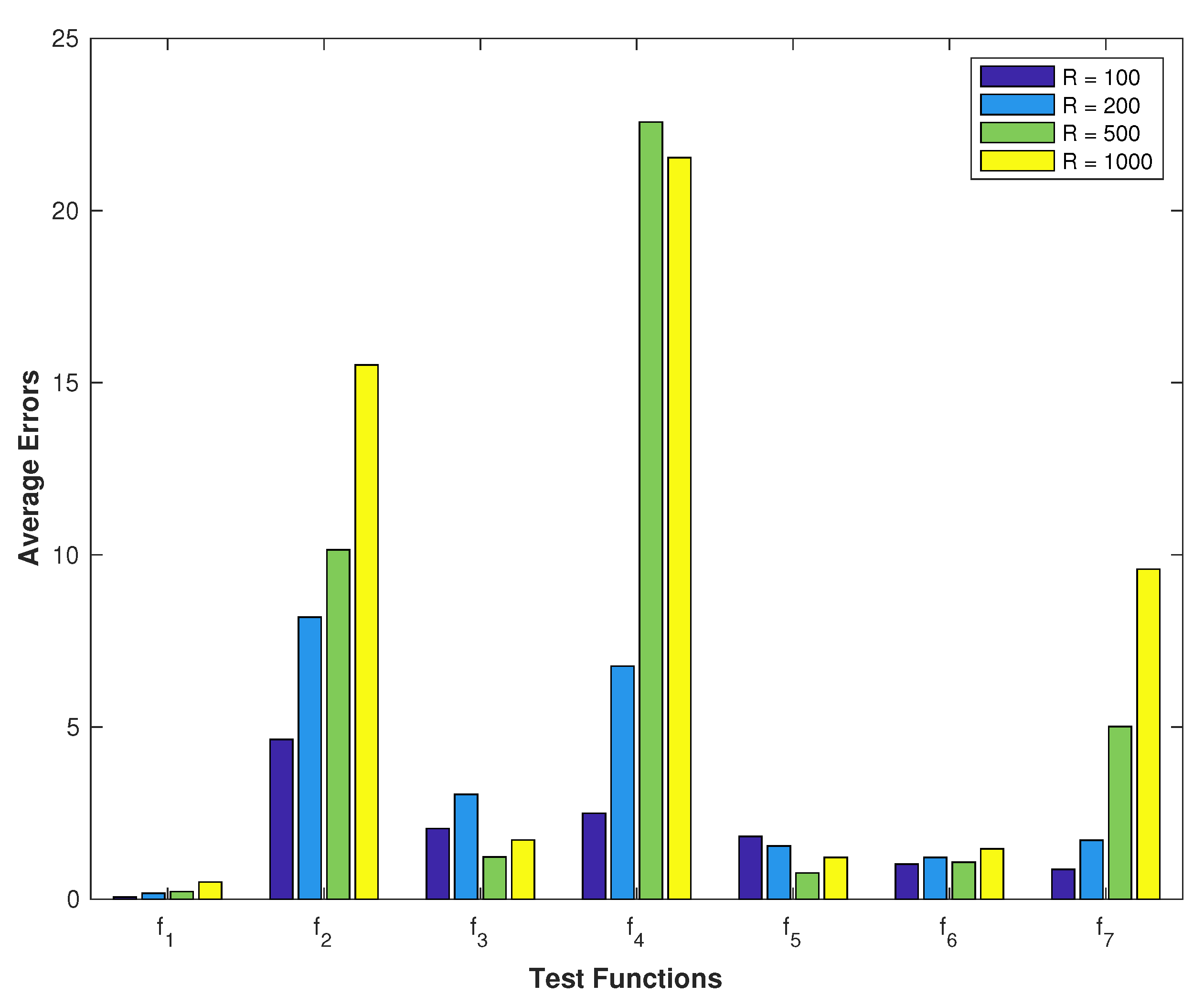
Before choosing a suitable value for parameter R, a comparison between different values of $R=100$, $R=200$, and $R=500$ was applied for both types of problems (global optimization, simulation-based optimization). The number of function evaluations was set to be fixed at 500,000 in all of these experiments.

Table 2. Average errors using different settings of parameter R for global optimization problems using Test Set A.

f	$\mathit{R}=100$	$\mathit{R}=200$	$\mathit{R}=500$
$RC$	$3.58\times {10}^{-7}$	$3.58\times {10}^{-7}$	$1.42\times {10}^{-4}$
$GP$	$7.82\times {10}^{-14}$	$7.80\times {10}^{-14}$	$7.80\times {10}^{-14}$
$R_2$	$2.90\times {10}^{-3}$	$3.14\times {10}^{-5}$	$1.92\times {10}^{-2}$
$H_{3,4}$	$2.15\times {10}^{-6}$	$2.15\times {10}^{-6}$	$2.15\times {10}^{-6}$
$S_{4,7}$	$5.66\times {10}^{-7}$	$5.66\times {10}^{-7}$	$5.66\times {10}^{-7}$
$P_{4,0.5}$	$1.07\times {10}^{-1}$	$4.54\times {10}^{-1}$	$7.06\times {10}^{-1}$
$T_6$	$2.50\times {10}^{-3}$	$4.04\times {10}^{-1}$	$8.50\times {10}^{-5}$
$R{T}_{10}$	$3.27\times {10}^{-13}$	$0.00$	$1.80\times {10}^{-3}$
$R_{10}$	$5.40\times {10}^{-1}$	$7.99\times {10}^{-1}$	$1.85$
$R{T}_{20}$	$8.57\times 10$	$7.70\times 10$	$9.77\times 10$
$R_{20}$	$7.38$	$8.36$	$8.94$
$P{W}_{24}$	$2.05\times {10}^{-10}$	$3.22\times {10}^{-9}$	$2.22\times {10}^{-3}$
$D{P}_{25}$	$6.80\times {10}^{-1}$	$7.99\times {10}^{-1}$	$9.06\times {10}^{-1}$
$A{K}_{30}$	$4.44\times {10}^{-15}$	$3.03\times {10}^{-12}$	$3.44\times {10}^{-4}$

shows that for the global optimization problem, increasing the population size does not have a positive effect on most problems. This means that the search process is more qualified with an extra number of generations. For the simulation-based optimization problem, Figure 1 shows an almost identical performance when applying different values of $R=100$, $R=200$, $R=500$, and $R=1000$. Some functions need more exploration of the search space (increase R), such as $f_3$ and $f_5$, but $R=100$ is still the best choice for rest of the functions.

For parameters m and L, which follow parameter R, setting higher values yields higher computational times without any significant improvement. For sample size parameters, the settings follow the recommended values in [10,13].

4.2. Global Optimization Results

The proposed DEDA algorithm was tested to solve nonlinear programming problems using the test functions in Set A and Set B. These test functions have diverse characteristics to assess various difficulties that occur in global optimization problems. For all test results for global optimizations, the records were obtained over 100 independent runs with a maximum function evaluation of 20,000. First,

Table 3. The deterministic Estimation of Distribution Algorithm (DEDA) results using Test Set B.

No.	f	Av.	Std.	No.	f	Av.	Std.
1	$RC$	$3.58\times {10}^{-7}$	$0.00$	2	$B_2$	$0.00$	$0.00$
3	$ES$	$3.86\times {10}^{-12}$	$0.00$	4	$GP$	$7.82\times {10}^{-14}$	$0.00$
5	$SH$	$1.48\times {10}^{-1}$	$1.51$	6	$BL$	$3.73\times {10}^{-15}$	$7.30\times {10}^{-15}$
7	$BO$	$0.00$	$0.00$	8	$MT$	$2.34\times {10}^{-27}$	$5.21\times {10}^{-25}$
9	$HM$	$8.65\times {10}^{-8}$	$0.00$	10	$S{C}_2$	$2.16\times {10}^7$	$4.48\times {10}^7$
11	$R_2$	$7.69\times {10}^{-5}$	$5.91\times {10}^{-3}$	12	$Z_2$	$1.88\times {10}^{-130}$	$2.40\times {10}^{-44}$
13	$DJ$	$9.77\times {10}^{-114}$	$9.33\times {10}^{-114}$	14	$H_{3,4}$	$2.15\times {10}^{-60}$	$0.00$
15	$CV$	$2.35\times {10}^{-4}$	$1.09\times {10}^{-1}$	16	$S_{4,5}$	$2.21\times {10}^{-7}$	$0.00$
17	$S_{4,7}$	$5.69\times {10}^{-7}$	$7.49\times {10}^{-16}$	18	$S_{4,10}$	$9.82\times {10}^{-6}$	$0.00$
19	$P_{4,0.5}$	$7.69\times {10}^{-1}$	$6.14\times {10}^{-1}$	20	$P_{4,0.5}^0$	$3.64\times {10}^{-2}$	$2.19\times {10}^{-2}$
21	$P{S}_{8,18,44,114}$	$3.81\times {10}^{-1}$	$3.53\times {10}^{-2}$	22	$H_{6,4}$	$1.96\times {10}^{-6}$	$2.35\times {10}^{-13}$
23	$S{C}_8$	$1.39\times {10}^9$	$2.51\times {10}^9$	24	$T_6$	$2.13\times {10}^{-1}$	$9.44\times {10}^{-1}$
25	$T_{10}$	$5.76\times 10$	$1.58$	26	$R{T}_{10}$	$2.50\times 10$	$8.18$
27	$G_{10}$	$0.00$	$0.00$	28	$S{S}_{10}$	$6.16\times {10}^{-50}$	$9.56\times {10}^{-50}$
29	$R_{10}$	$1.88$	$9.97\times {10}^{-1}$	30	$Z_{10}$	$5.25\times {10}^{-3}$	$4.20\times {10}^{-3}$
31	$R{T}_{20}$	$8.44\times {10}^{-12}$	$7.04\times {10}^{-50}$	32	$G_{20}$	$0.00$	$0.00$
33	$S{S}_{20}$	$4.32\times {10}^{-24}$	$1.89\times {10}^{-29}$	34	$R_{20}$	$7.55$	$6.27\times {10}^{-1}$
35	$Z_{20}$	$1.98\times {10}^{-1}$	$1.62\times {10}^{-1}$	36	$P{W}_{24}$	$5.33\times {10}^{-8}$	$1.27\times {10}^{-7}$
37	$D{P}_{25}$	$8.15\times {10}^{-1}$	$5.01\times {10}^{-2}$	38	$L_{30}$	$1.06\times {10}^{-22}$	$5.12\times {10}^{-23}$
39	$S{R}_{30}$	$3.16\times {10}^{-25}$	$1.78\times {10}^{-25}$	40	$A{K}_{30}$	$3.78\times {10}^{-12}$	$5.89\times {10}^{-13}$

shows average errors (Av.) and standard deviation (Std.) obtained by the DEDA method using Test Set B. It reached the global optima within error gaps less than ${10}^{-3}$ for 25 out of 40 test functions.

The DEDA results were compared with those of the scatter search methods introduced in [10]:

• Scatter Search (SS): The standard scatter search method.
• Directed Scatter Search (DSS): An SS-based method directed by a memory-based element called gene matrix in order to increase the search diversity.

Table 4. Compared results of the DEDA, SS, and DSS methods using Test Set A.

	SS			DSS			DEDA
$\mathbf{f}$	Av.	Std.	Suc.	Av.	Std.	Suc.	Av.	Std.	Suc.
$RC$	$3.58\times {10}^{-7}$	$8.48\times {10}^{-10}$	100	$3.58\times {10}^{-7}$	$5.83\times {10}^{-10}$	100	$3.58\times {10}^{-7}$	$0.00$	100
$GP$	$4.69\times {10}^{-11}$	$1.85\times {10}^{-6}$	100	$5.35\times {10}^{-11}$	$7.65\times {10}^{-9}$	100	$7.82\times {10}^{-14}$	$0.00$	100
$R_2$	$1.10\times {10}^{-11}$	$3.68\times {10}^{-10}$	100	$2.56\times {10}^{-11}$	$1.22\times {10}^{-9}$	100	$7.69\times {10}^{-5}$	$5.91\times {10}^{-3}$	100
$H_{3,4}$	$2.11\times {10}^{-6}$	$2.71\times {10}^{-9}$	100	$2.15\times {10}^{-6}$	$2.79\times {10}^{-9}$	100	$2.15\times {10}^{-6}$	$0.00$	100
$S_{4,7}$	$2.94\times {10}^{-7}$	$9.16\times {10}^{-8}$	100	$3.22\times {10}^{-7}$	$2.65\times {10}^{-7}$	100	$5.67\times {10}^{-7}$	$7.49\times {10}^{-16}$	100
$P_{4,0.5}$	$6.10\times {10}^{-1}$	$4.80\times {10}^{-2}$	13	$5.52\times {10}^{-1}$	$5.90\times {10}^{-3}$	27	$1.07\times {10}^{-1}$	$2.19\times {10}^{-2}$	0
$T_6$	$2.39\times {10}^{-3}$	$8.87\times {10}^{-4}$	80	$2.70\times {10}^{-3}$	$3.01\times {10}^{-3}$	77	$2.52\times {10}^{-3}$	$9.44\times {10}^{-1}$	0
$R{T}_{10}$	$4.66\times {10}^{-6}$	$1.29\times {10}^{-6}$	100	$1.92\times {10}^{-6}$	$4.34\times {10}^{-7}$	100	$3.27\times {10}^{-13}$	$8.18$	100
$R_{10}$	$1.85\times 10$	$3.59$	0	$1.50\times 10$	$1.69$	0	$5.42\times {10}^{-1}$	$9.97\times {10}^{-1}$	0
$R{T}_{20}$	$3.56$	$1.10$	0	$5.01$	$7.88\times {10}^{-1}$	0	$8.43$	$7.04\times {10}^{-50}$	0
$R_{20}$	$4.58\times 10$	$2.79\times 10$	0	$2.98\times 10$	$2.13\times 10$	0	$7.55$	$6.27\times {10}^{-1}$	0
$P{W}_{24}$	$4.71\times 10$	$2.11\times 10$	0	$1.62\times 10$	$7.67$	0	$2.05\times {10}^{-10}$	$1.27\times {10}^{-7}$	100
$D{P}_{25}$	$3.51$	$2.68$	0	$1.43$	$2.31\times {10}^{-1}$	0	$6.80\times {10}^{-1}$	$5.01\times {10}^{-2}$	0
$A{K}_{30}$	$1.04\times 10$	$1.95$	0	$8.28$	$3.02$	0	$4.44\times {10}^{-15}$	$5.89\times {10}^{-13}$	100

shows the average errors (Av.), standard deviation (Std.) and success rates (Suc.) obtained by each method using Test Set A. In general, the DEDA obtained lower average errors and higher success rates than the other two methods, as can be seen in the ranks $R^{+}$ and $R^{-}$ in

Table 5. Wilcoxon rank-sum test for the results of Table 4.

Criterion	Methods	${\mathit{R}}^{+}$	${\mathit{R}}^{-}$	p-Value	Best Method
Average Errors	DEDA, SS	30.5	74.5	0.1982	–
	DEDA, DSS	21.5	83.5	0.2063	–
Success Rates	DEDA, SS	54.5	50.5	0.6995	–
	DEDA, DSS	54.5	50.5	0.6995	–

. However, there was no significant difference between these methods according to the p-values obtained by the Wilcoxon rank-sum test, as shown in Table 5.

4.3. Fuzzy Sampling Performance

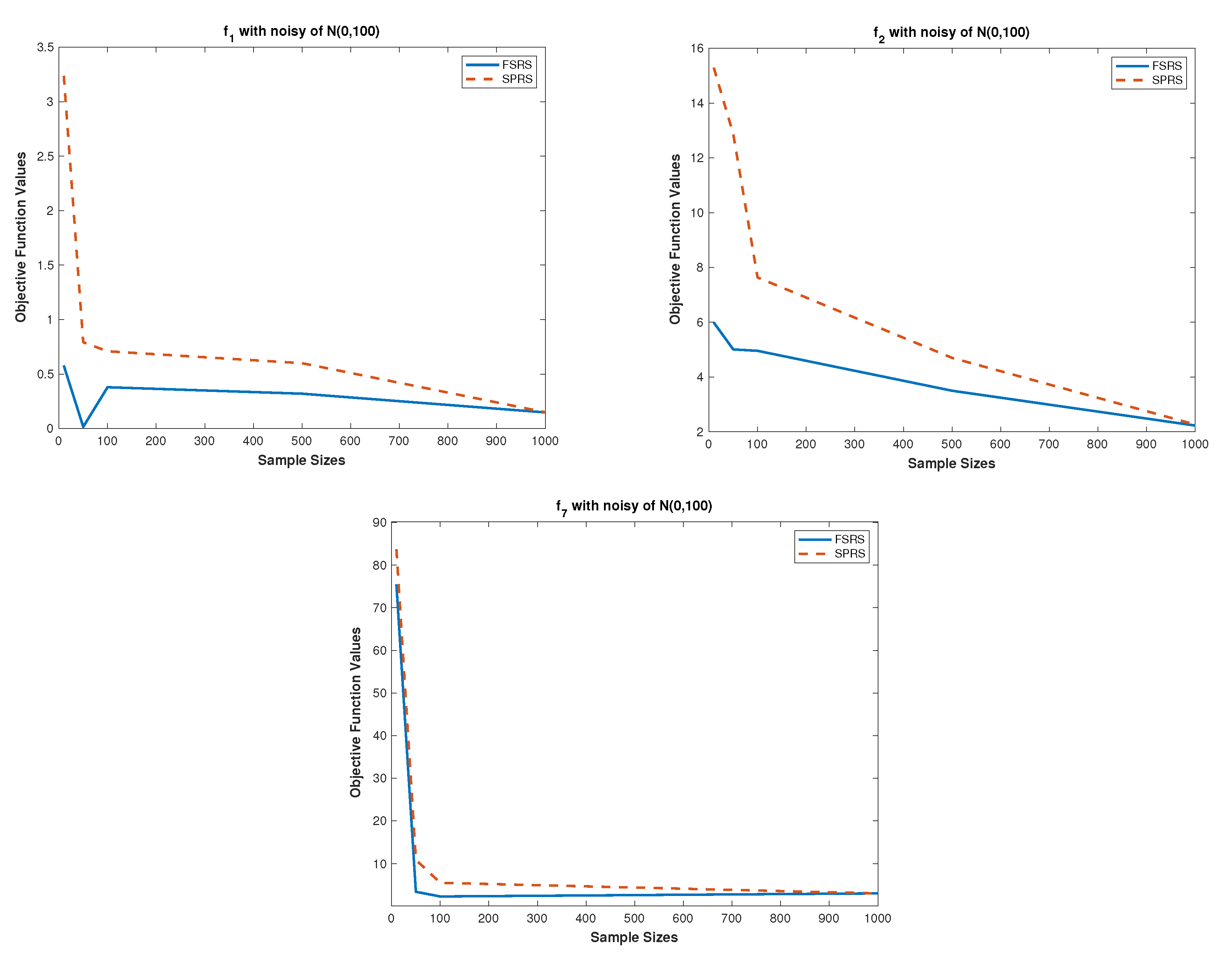
The FSRS (Algorithm 6) results were compared with those of the standard SPRS (Algorithm 5) in high noise—i.e., $N(0,{10}^2)$. These results are illustrated in Figure 2 which shows the average $\widehat{f}\left(x\right)$ of the best obtained solutions by each method for every test function. Tested functions with different dimensions were selected from Test Set C. The sample size varies from 10 to 1000. The results shown in Figure 2 reveal that the performance of the FSRS algorithm is consistently better than that of the SPRS algorithm for small number values N. There is no significant difference between them with higher sample sizes. Therefore, the proposed fuzzy sampling could efficiently deal with a wide range of noise, especially with small sample sizes.

4.4. Simulation-Based Optimization Results

In this section, we give more details about the experimental results of the comparison between the proposed FSEDA and ASEDA algorithms. Then, the results of the best method are compared with other benchmark methods.

Table 6. The best and average errors of the the Average Sampling Estimation of Distribution Algorithm (ASEDA) and FSDEA methods using Test Set C.

	ASEDA			FSEDA
$f$	Best	Av.	Std.	Best	Av.	Std.
$f_1$	$1.05\times {10}^{-2}$	$1.76\times {10}^{-1}$	$3.88\times {10}^{-2}$	$1.30\times {10}^{-2}$	$7.15\times {10}^{-2}$	$2.00\times {10}^{-1}$
$f_2$	$3.67$	$5.93$	$2.50$	$3.05$	$5.90$	$8.12\times {10}^{-1}$
$f_3$	$9.50\times {10}^{-1}$	$1.86$	$1.50$	$3.68\times {10}^{-1}$	$2.66$	$5.43\times {10}^{-1}$
$f_4$	$3.79$	$6.98$	$3.57$	$2.81$	$6.21$	$2.12$
$f_5$	$4.60\times {10}^{-1}$	$1.26$	$6.86\times {10}^{-1}$	$2.45\times {10}^{-1}$	$9.99\times {10}^{-1}$	$5.12\times {10}^{-1}$
$f_6$	$7.71\times {10}^{-1}$	$1.08$	$5.02\times {10}^{-1}$	$3.43\times {10}^{-1}$	$1.07$	$2.77\times {10}^{-1}$
$f_7$	$1.67$	$2.21$	$3.76\times {10}^{-1}$	$1.39$	$1.80$	$2.80\times {10}^{-1}$

shows the best and average errors obtained by the two methods using the seven test functions in Set C. The FSEDA method could obtain better solutions than the other method for six out of seven test functions, and its average solutions are better in five out of seven test functions. Therefore, we used the FSEDA results to compare with the other benchmark methods.

Two main comparison experiments are presented to test the FSEDA performance against some benchmark methods. The first experiment used Test Set C to make the comparisons with methods in [10,68], while the other experiment used Test Set D with methods in [12,13].

Table 7. The best and average errors of the FSDEA method compared with the DESSP and DSSSP methods.

	DESSP			DSSSP			FSDEA
$f$	Best	Average	Std.	Best	Average	Std.	Best	Average	Std.
$f_1$	$\mathbf{5}.\mathbf{02}\times {\mathbf{10}}^{-\mathbf{4}}$	$2.33\times {10}^{-1}$	$1.06$	$1.46\times {10}^{-2}$	$2.94\times {10}^{-1}$	$2.97\times {10}^{-1}$	$1.30\times {10}^{-2}$	$\mathbf{7}.\mathbf{15}\times {\mathbf{10}}^{-\mathbf{2}}$	$2.00\times {10}^{-1}$
$f_2$	$8.05\times {10}^{-1}$	$\mathbf{3}.\mathbf{55}$	$1.37$	$\mathbf{4}.\mathbf{08}\times {\mathbf{10}}^{-\mathbf{1}}$	$6.56$	$3.74$	$3.05$	$5.90$	$8.12\times {10}^{-1}$
$f_3$	$\mathbf{1}.\mathbf{05}\times {\mathbf{10}}^{-\mathbf{3}}$	$\mathbf{3}.\mathbf{31}\times {\mathbf{10}}^{-\mathbf{1}}$	$4.98\times {10}^{-1}$	$5.90\times {10}^{-1}$	$1.04$	$2.92\times {10}^{-1}$	$3.68\times {10}^{-1}$	$2.66$	$5.43\times {10}^{-1}$
$f_4$	$\mathbf{1}.\mathbf{44}\times {\mathbf{10}}^{-\mathbf{1}}$	$\mathbf{3}.\mathbf{75}$	$5.96$	$2.75$	$6.71$	$3.97$	$2.81$	$6.21$	$2.12$
$f_5$	$\mathbf{4}.\mathbf{13}\times {\mathbf{10}}^{-\mathbf{4}}$	$\mathbf{3}.\mathbf{87}\times {\mathbf{10}}^{-\mathbf{1}}$	$5.99\times {10}^{-1}$	$2.82\times {10}^{-1}$	$1.91$	$6.50\times {10}^{-1}$	$2.45\times {10}^{-1}$	$9.99\times {10}^{-1}$	$5.12\times {10}^{-1}$
$f_6$	$\mathbf{1}.\mathbf{24}\times {\mathbf{10}}^{-\mathbf{5}}$	$\mathbf{2}.\mathbf{13}\times {\mathbf{10}}^{-\mathbf{2}}$	$7.68\times {10}^{-2}$	$3.85\times {10}^{-4}$	$9.21\times {10}^{-2}$	$9.31\times {10}^{-2}$	$3.43\times {10}^{-1}$	$1.07$	$2.77\times {10}^{-1}$
$f_7$	$2.79\times 10$	$3.96\times 10$	$5.67$	$8.41$	$1.24\times 10$	$2.64$	$\mathbf{1}.\mathbf{39}$	$\mathbf{1}.\mathbf{80}$	$2.80\times {10}^{-1}$

shows the best and the average errors obtained by the proposed FSEDA method and the following evolutionary-based methods:

• DESSP: Directed evolution strategies for stochastic programming [10].
• DSSSP: Directed scatter search for stochastic programming [10,68].

The results were obtained over 25 independent runs with maximum function evaluations equal to 500,000. Moreover,

Table 8. Wilcoxon rank-sum test for the results of Table 7.

Criterion	Methods	${\mathit{R}}^{+}$	${\mathit{R}}^{-}$	p-Value	Best Method
Best Solutions	FSDEA, DESSP	21	7	0.1282	–
	FSDEA, DSSSP	14	14	0.9015	–
Average Errors	FSDEA, DESSP	20	8	0.6200	–
	FSDEA, DSSSP	11	17	0.6200	–

shows the statistical measures of the results compared in Table 7. These statistical measures reveal that there is no significant difference between the proposed method and the other two methods in terms of the best solution found or the average errors. However, for high dimensional function $f_7$, the proposed method demonstrated the best performance.

The other comparison experiment compared the FSEDA results with those of the following benchmark methods [12,13] using Test Set D with dimensions 30 and 100.

• EDA–MMSS: An EDA-based method with a modified sampling search mechanism called min–max sampling [13].
• DE/rand/1: A modified version of the standard differential evolution of DE/rand/1/bin algorithm [12].
• jDE: An adaptive differential evolution method [69].
• GADS: Genetic algorithm with duration sizing [70].
• DERSFTS: Differential evolution with randomized scale factor and threshold-based selection [71].
• OBDE: Opposition-based differential evolution [72].
• NADE: Noise analysis differential evolution [73].
• MUDE: Memetic differential evolution for noisy optimization [74].
• MDE–DS: Modified differential evolution with a distance-based selection [12].
• NRDE: Noise resilient differential evolution [75].

The average errors over 30 independent runs are reported in the following tables, with computational budgets of 100,000 and 300,000 function evaluations for dimensions 30 and 100, respectively.

Table 9. Average errors obtained by the compared methods for Test Set D with $n=30$, and 100,000 maximum function evaluations.

	FSEDA		EDA-MMSS		DE/rand/1		jDE		GADS
$\mathbf{g}$	Av.	Std.	Av.	Std.	Av.	Std.	Av.	Std.	Av.	Std.
$g_1$	$6.82\times {10}^{-2}$	$2.00\times {10}^{-2}$	$5.60\times {10}^{-1}$	$1.75\times {10}^{-1}$	$3.67$	$3.26\times {10}^{-2}$	$4.59\times {10}^{-1}$	$7.41\times {10}^{-2}$	$1.95$	$2.26\times {10}^{-1}$
$g_2$	$6.48\times {10}^{-2}$	$3.71\times {10}^{-2}$	$8.54$	$2.26$	$5.89\times 10$	$1.10\times 10$	$4.25\times 10$	$7.54$	$3.24\times 10$	$1.88\times 10$
$g_3$	$3.88\times {10}^{-2}$	$1.20\times {10}^{-2}$	$9.25$	$3.39$	$6.56\times {10}^3$	$1.65\times {10}^3$	$4.27\times {10}^3$	$1.08\times {10}^3$	$7.44\times {10}^3$	$3.89\times {10}^3$
$g_4$	$3.20\times {10}^{-2}$	$1.34\times {10}^{-2}$	$4.14$	$9.84\times {10}^{-1}$	$1.02\times {10}^2$	$2.71\times 10$	$5.82\times 10$	$1.82\times 10$	$6.49\times 10$	$3.54\times 10$
$g_5$	$4.05\times {10}^{-3}$	$6.49\times {10}^{-4}$	$2.82\times {10}^{-1}$	$1.08\times {10}^{-1}$	$9.98\times {10}^{-3}$	$7.58\times {10}^{-3}$	$7.67\times {10}^{-1}$	$6.55\times {10}^{-2}$	$2.76\times {10}^{-2}$	$1.06\times {10}^{-2}$
$g_6$	$8.21\times {10}^{-1}$	$1.16\times {10}^{-1}$	$2.42$	$3.53\times {10}^{-1}$	$4.18\times {10}^2$	$7.79\times 10$	$1.99\times {10}^2$	$4.28\times 10$	$4.75\times {10}^2$	$2.48\times {10}^2$
$g_7$	$9.73$	$3.00$	$2.28\times 10$	$2.08$	$6.34$	$2.07$	$2.08\times 10$	$2.04$	$1.29\times 10$	$1.06$
$g_8$	$2.40\times {10}^{-2}$	$1.02\times {10}^{-2}$	$3.73\times 10$	$3.24\times 10$	$1.65\times {10}^4$	$4.30\times {10}^3$	$9.19\times {10}^3$	$2.06\times {10}^3$	$1.05\times {10}^4$	$6.43\times {10}^3$
$g_9$	$1.29\times 10$	$1.04$	$1.12\times 10$	$8.01\times {10}^{-1}$	$5.74$	$5.60\times {10}^{-1}$	$4.65$	$1.31$	$3.81$	$2.12$
$g_{10}$	$1.85\times {10}^2$	$5.53\times 10$	$4.26\times 10$	$1.51\times 10$	$3.91\times {10}^2$	$6.50\times 10$	$2.90\times {10}^2$	$3.82\times 10$	$2.31\times {10}^2$	$6.27\times 10$
$g_{11}$	$2.36\times 10$	$1.73$	$4.37\times 10$	$8.79$	$6.36\times {10}^3$	$2.09\times {10}^3$	$4.12\times {10}^3$	$1.68\times {10}^3$	$7.50\times {10}^3$	$2.12\times {10}^3$
$g_{12}$	$2.46\times {10}^4$	$4.04\times {10}^3$	$4.51\times {10}^3$	$2.95\times {10}^3$	$7.89\times {10}^3$	$5.77\times {10}^2$	$8.22\times {10}^3$	$9.54\times {10}^2$	$6.09\times {10}^3$	$1.03\times {10}^3$
$g_{13}$	$1.12$	$2.46\times {10}^{-1}$	$6.19\times {10}^{-1}$	$2.31\times {10}^{-1}$	$1.18$	$3.02\times {10}^{-1}$	$9.91\times {10}^{-1}$	$3.19\times {10}^{-1}$	$1.46$	$5.39\times {10}^{-1}$
	DERSFTS		OBDE		NADE		MUDE		MDE-DS
$\mathbf{g}$	Av.	Std.	Av.	Std.	Av.	Std.	Av.	Std.	Av.	Std.
$g_1$	$1.10$	$4.77\times {10}^{-1}$	$3.35$	$3.40\times {10}^{-1}$	$2.99\times {10}^{-1}$	$8.88\times {10}^{-2}$	$2.59\times {10}^{-1}$	$6.99\times {10}^{-2}$	$0.00$	$0.00$
$g_2$	$5.67\times 10$	$9.79$	$5.69\times 10$	$1.13\times 10$	$3.29\times 10$	$6.70$	$2.69\times 10$	$6.98$	$8.53\times {10}^{-3}$	$2.84\times {10}^{-2}$
$g_3$	$6.84\times {10}^3$	$2.21\times {10}^3$	$8.23\times {10}^3$	$1.85\times {10}^3$	$3.32\times {10}^3$	$1.17\times {10}^3$	$2.36\times {10}^3$	$1.06\times {10}^3$	$7.08\times {10}^{-4}$	$8.56\times {10}^{-5}$
$g_4$	$1.06\times {10}^2$	$3.61\times 10$	$1.45\times {10}^2$	$2.68\times 10$	$4.53\times 10$	$2.14\times 10$	$3.68\times 10$	$1.33\times 10$	$7.92\times {10}^{-2}$	$2.56\times {10}^{-6}$
$g_5$	$7.84\times {10}^{-1}$	$5.88\times {10}^{-2}$	$4.16\times {10}^{-2}$	$2.51\times {10}^{-2}$	$8.30\times {10}^{-1}$	$6.87\times {10}^{-2}$	$7.69\times {10}^{-1}$	$4.65\times {10}^{-2}$	$5.41\times {10}^{-4}$	$9.45\times {10}^{-8}$
$g_6$	$3.95\times {10}^2$	$1.37\times {10}^2$	$5.21\times {10}^2$	$7.50\times 10$	$1.65\times {10}^2$	$6.29\times 10$	$1.46\times {10}^2$	$4.45\times 10$	$1.41\times {10}^{-3}$	$1.01$
$g_7$	$8.52$	$2.30$	$9.27$	$1.97$	$2.46\times 10$	$1.35$	$2.32\times 10$	$1.27$	$2.02$	$5.45$
$g_8$	$1.66\times {10}^4$	$4.53\times {10}^3$	$2.15\times {10}^4$	$4.89\times {10}^3$	$6.84\times {10}^3$	$1.79\times {10}^3$	$5.28\times {10}^3$	$2.12\times {10}^3$	$7.81\times {10}^{-1}$	$2.21\times {10}^{-1}$
$g_9$	$3.92$	$1.40$	$4.25$	$8.73\times {10}^{-1}$	$5.05$	$1.16$	$5.41$	$1.36$	$1.39$	$2.15$
$g_{10}$	$3.83\times {10}^2$	$5.63\times 10$	$3.78\times {10}^2$	$4.66\times 10$	$1.96\times {10}^2$	$5.00\times 10$	$2.00\times {10}^2$	$4.30\times 10$	$1.89\times {10}^{-2}$	$2.34\times {10}^{-1}$
$g_{11}$	$6.12\times {10}^3$	$3.03\times {10}^3$	$7.26\times {10}^3$	$2.18\times {10}^3$	$3.76\times {10}^3$	$2.28\times {10}^3$	$2.49\times {10}^3$	$1.71\times {10}^3$	$2.60\times 10$	$2.32$
$g_{12}$	$1.01\times {10}^4$	$8.28\times {10}^2$	$8.03\times {10}^3$	$5.42\times {10}^2$	$5.60\times {10}^3$	$8.80\times {10}^2$	$6.00\times {10}^3$	$9.99\times {10}^2$	$0.00$	$0.00$
$g_{13}$	$5.89\times {10}^{-1}$	$3.01\times {10}^{-1}$	$1.08$	$2.99\times {10}^{-1}$	$1.82$	$2.52\times {10}^{-1}$	$1.57$	$2.80\times {10}^{-1}$	$1.03\times 10$	$4.23$

displays the average errors for test functions with $n=30,$ and the statistical measures of these results are presented in

Table 10. Wilcoxon rank-sum test for the results of Table 9.

Criterion	Methods	${\mathit{R}}^{+}$	${\mathit{R}}^{-}$	p-Value	Best Method
Average Errors	FSEDA, EDA–MMSS	33	58	0.1370	–
	FSEDA, DE/rand/1	21	70	0.0313	FSEDA
	FSEDA, jDE	18	73	0.0183	FSEDA
	FSEDA, GADS	18	73	0.0225	FSEDA
	FSEDA, DERSFTS	22	69	0.0240	FSEDA
	FSEDA, OBDE	22	69	0.0240	FSEDA
	FSEDA, NADE	17	74	0.0138	FSEDA
	FSEDA, MUDE	17	74	0.0183	FSEDA
	FSEDA, MDE–DS	64	27	0.0812	–

. The FSEDA outperforms seven out of nine methods in terms of obtaining better average solutions.

The results of test functions with $n=100$ are shown in

Table 11. Average errors obtained by the compared methods for Test Set D with $n=100$, and 300,000 maximum function evaluations.

	FSEDA		DE/rand/1		jDE		GADS		DERSFTS
$\mathbf{g}$	Av.	Std.	Av.	Std.	Av.	Std.	Av.	Std.	Av.	Std.
$g_1$	$1.71\times {10}^{-1}$	$6.15\times {10}^{-2}$	$3.67$	$1.18\times {10}^{-2}$	$8.13\times {10}^{-1}$	$1.31\times {10}^{-1}$	$3.01$	$8.21\times {10}^{-2}$	$1.34$	$1.81\times {10}^{-1}$
$g_2$	$2.09$	$5.63\times {10}^{-1}$	$1.71\times {10}^2$	$1.86\times 10$	$1.36\times {10}^2$	$1.54\times 10$	$1.52\times {10}^2$	$1.43\times 10$	$1.64\times {10}^2$	$1.86\times 10$
$g_3$	$1.89\times {10}^{-1}$	$7.82\times {10}^{-2}$	$7.89\times {10}^4$	$8.59\times {10}^3$	$4.17\times {10}^4$	$6.64\times {10}^3$	$8.35\times {10}^4$	$2.67\times {10}^4$	$4.98\times {10}^4$	$1.22\times {10}^4$
$g_4$	$9.02\times {10}^{-2}$	$2.51\times {10}^{-2}$	$4.03\times {10}^2$	$6.03\times 10$	$2.01\times {10}^2$	$2.95\times 10$	$3.87\times {10}^2$	$3.90\times 10$	$2.35\times {10}^2$	$4.45\times 10$
$g_5$	$4.57\times {10}^{-4}$	$8.43\times {10}^{-3}$	$3.29\times {10}^{-3}$	$1.74\times {10}^{-3}$	$1.44\times {10}^{-1}$	$4.27\times {10}^{-2}$	$4.85\times {10}^{-3}$	$5.85\times {10}^{-4}$	$2.26\times {10}^{-1}$	$6.38\times {10}^{-2}$
$g_6$	$1.09$	$1.65\times {10}^{-1}$	$1.48\times {10}^3$	$1.91\times {10}^2$	$7.29\times {10}^2$	$1.06\times {10}^2$	$1.43\times {10}^3$	$2.36\times {10}^2$	$8.43\times {10}^2$	$2.09\times {10}^2$
$g_7$	$1.93\times 10$	$5.84$	$1.04\times 10$	$1.99$	$5.81\times 10$	$3.41$	$1.80\times 10$	$1.12$	$2.98\times 10$	$5.34$
$g_8$	$2.06\times {10}^{-1}$	$1.87\times {10}^{-1}$	$2.18\times {10}^5$	$3.05\times {10}^4$	$1.00\times {10}^5$	$1.56\times {10}^4$	$2.05\times {10}^5$	$4.21\times {10}^4$	$1.36\times {10}^5$	$3.55\times {10}^4$
$g_9$	$4.65\times 10$	$3.32$	$1.53\times 10$	$2.08$	$1.04\times 10$	$3.18$	$2.48\times 10$	$3.89$	$9.37$	$3.91$
$g_{10}$	$9.19\times {10}^2$	$3.25\times {10}^2$	$1.21\times {10}^3$	$1.02\times {10}^2$	$1.08\times {10}^3$	$7.29\times 10$	$1.15\times {10}^3$	$6.02\times 10$	$1.18\times {10}^3$	$7.04\times 10$
$g_{11}$	$9.09\times 10$	$1.83\times 10$	$2.03\times {10}^4$	$3.06\times {10}^3$	$1.00\times {10}^4$	$2.52\times {10}^3$	$2.28\times {10}^4$	$1.01\times {10}^4$	$1.21\times {10}^4$	$3.78\times {10}^3$
$g_{12}$	$4.45\times {10}^5$	$1.63\times {10}^5$	$2.68\times {10}^4$	$1.17\times {10}^3$	$3.97\times {10}^4$	$1.81\times {10}^3$	$2.88\times {10}^4$	$1.07\times {10}^3$	$3.18\times {10}^4$	$1.35\times {10}^3$
$g_{13}$	$6.03\times {10}^{-1}$	$2.98\times {10}^{-1}$	$1.03$	$2.02\times {10}^{-1}$	$6.82\times {10}^{-1}$	$1.54\times {10}^{-1}$	$1.13$	$1.74\times {10}^{-1}$	$4.61\times {10}^{-1}$	$1.76\times {10}^{-1}$
	OBDE		NADE		MUDE		NRDE		MDE-DS
$\mathbf{g}$	Av.	Std.	Av.	Std.	Av.	Std.	Av.	Std.	Av.	Std.
$g_1$	$3.61$	$2.08\times {10}^{-2}$	$3.65\times {10}^{-1}$	$1.04\times {10}^{-1}$	$3.35\times {10}^{-1}$	$7.49\times {10}^{-2}$	$0.00$	$0.00$	$0.00$	$0.00$
$g_2$	$1.99\times {10}^2$	$2.44\times 10$	$7.82\times 10$	$1.55\times 10$	$6.18\times 10$	$9.87$	$1.25$	$6.36\times {10}^{-1}$	$6.46\times {10}^{-1}$	$5.21$
$g_3$	$1.02\times {10}^5$	$1.35\times {10}^4$	$3.15\times {10}^4$	$7.64\times {10}^3$	$2.61\times {10}^4$	$7.26\times {10}^3$	$2.61$	$2.79$	$4.41\times {10}^{-1}$	$8.48\times {10}^{-1}$
$g_4$	$5.59\times {10}^2$	$7.46\times 10$	$1.24\times {10}^2$	$3.30\times 10$	$1.06\times {10}^2$	$2.16\times 10$	$5.91\times {10}^{-1}$	$5.03\times {10}^{-1}$	$6.68\times {10}^{-2}$	$1.24\times {10}^{-2}$
$g_5$	$5.79\times {10}^{-3}$	$8.33\times {10}^{-4}$	$3.75\times {10}^{-1}$	$8.11\times {10}^{-2}$	$1.70\times {10}^{-1}$	$4.36\times {10}^{-2}$	$1.54\times {10}^{-3}$	$6.03\times {10}^{-2}$	$4.82\times {10}^{-4}$	$2.45$
$g_6$	$2.00\times {10}^3$	$2.19\times {10}^2$	$4.50\times {10}^2$	$1.55\times {10}^2$	$4.00\times {10}^2$	$1.05\times {10}^2$	$1.76$	$7.00\times {10}^{-1}$	$7.73\times {10}^{-2}$	$4.54\times {10}^{-1}$
$g_7$	$1.85\times 10$	$2.77$	$6.53\times 10$	$3.43$	$7.20\times 10$	$2.22$	$7.10$	$1.34$	$1.24$	$2.14\times {10}^{-1}$
$g_8$	$2.92\times {10}^5$	$4.01\times {10}^4$	$6.60\times {10}^4$	$1.89\times {10}^4$	$6.11\times {10}^4$	$1.82\times {10}^4$	$1.09$	$1.53$	$3.69\times {10}^{-2}$	$1.45$
$g_9$	$7.65$	$2.98$	$1.29\times 10$	$2.03$	$1.28\times 10$	$2.26$	$4.85\times 10$	$5.78\times {10}^{-2}$	$6.22$	$1.21$
$g_{10}$	$1.34\times {10}^3$	$1.43\times {10}^2$	$5.01\times {10}^2$	$8.09\times 10$	$5.80\times {10}^2$	$8.04\times 10$	$1.35\times {10}^{-1}$	$1.09\times {10}^{-1}$	$1.54\times {10}^{-2}$	$4.75\times {10}^{-3}$
$g_{11}$	$2.83\times {10}^4$	$5.26\times {10}^3$	$8.18\times {10}^3$	$3.20\times {10}^3$	$7.16\times {10}^3$	$2.46\times {10}^3$	$1.07\times {10}^2$	$2.16\times 10$	$9.45\times 10$	$2.78$
$g_{12}$	$2.78\times {10}^4$	$1.19\times {10}^3$	$1.96\times {10}^4$	$1.64\times {10}^3$	$2.06\times {10}^4$	$1.74\times {10}^3$	$0.00$	$0.00$	$0.00$	$0.00$
$g_{13}$	$8.49\times {10}^{-1}$	$1.76\times {10}^{-1}$	$1.78$	$1.12\times {10}^{-1}$	$1.57$	$1.90\times {10}^{-1}$	$1.97\times 10$	$2.46$	$1.86\times 10$	$5.46\times {10}^{-1}$

. Their statistical measures are reported in

Table 12. Wilcoxon rank-sum test for the results of Table 11.

Criterion	Methods	${\mathit{R}}^{+}$	${\mathit{R}}^{-}$	p-Value	Best Method
Average Errors	FSEDA, DE/rand/1	22	69	0.0402	FSEDA
	FSEDA, jDE	17	74	0.0402	FSEDA
	FSEDA, GADS	21	70	0.0313	FSEDA
	FSEDA, DERSFTS	19	72	0.0313	FSEDA
	FSEDA, OBDE	21	70	0.0402	FSEDA
	FSEDA, NADE	25	66	0.0355	FSEDA
	FSEDA, MUDE	25	66	0.0513	–
	FSEDA, NRDE	41	50	0.6260	–
	FSEDA, MDE–DS	68	23	0.0812	–

. The FSEDA method outperformed six out of nine methods used in this comparison in terms of average solution quality.

5. Stochastic Programming Applications

In this section, we investigate the strength of the proposed methods in solving real-world problems. Therefore, the FSEDA and ASEDA methods attempted to find the best solutions for three different real stochastic programming applications:

• The product mix (PROD-MIX) problem [76,77];
• The modified production planning Kall and Wallace (KANDW3) problem [77,78];
• The two-stage optimal capacity investment Louveaux and Smeers (LANDS) problem [77,79].

These applications are constrained stochastic programming problems. Therefore, the penalty methodology [80] was used to transform these constrained problems into a series of unconstrained ones. These unconstrained solutions are assumed to converge to the solutions of the corresponding constrained problem.

To solve these problems, the proposed EDA-based methods were used with the parameters in Table 1, except the population size, which was adjusted to $R=300$. The penalty parameter was set to $\lambda =1000$. The algorithms were terminated when they reached $30,000$ function evaluations.

5.1. PROD-MIX Problem

This problem assumes that a furniture shop has two workstations $(j=1,2)$; the first workstation is for carpentry and the other for finishing. The furniture shop has four products $(i=1,\dots ,4)$. Each product i consumes a certain number of man-hours $t_{ij}$ at j a workstation, with man-hours $h_j$ being limited at each workstation j. The shop should purchase man-hours $v_j$ from outside the workstation j if the man-hours exceed the limit. Each product earns a certain profit $c_i$. The most important aspect is to maximize the total profit of our shop and minimize the cost of purchased man-hours.

5.1.1. The Mathematical Formulation of the PROD-MIX Problem

The formal description of the PROD-MIX Problem can be defined as follows [76,77]. The required values for parameters and constants are also expressed.

i	The product class ($i=1,\dots ,4$).
j	The workstation ($j=1,2$).
$x_i$	The quantities of product (decision variables).
$v_j$	The outside purchased man-hours for workstation j.
$c_i$	The profit per product unit at class i, $c=[12.0,20.0,18.0,40.0]$.
$q_j$	The man-hour cost for workstation j, $q=[5.0,10.0].$
$t_{ij}$	Random man-hours at workstation j per unit of product class i,
	$t=\left[\begin{array}{cccc}U(3.5,4.5)& U(8.0,10.0)& U(6.0,8.0)& U(9.0,11.0)\\ U(0.8,1.2)& U(0.8,1.2)& U(2.5,3.5)& U(36.0,44.0)\end{array}\right].$
$h_i$	Random available man-hours at j workstation,
	$h=\left[N\right(6000,100),N(4000,50\left)\right]$.

Therefore, the object function for the PROD-MIX Problem can be expressed as

$$f(x,v)=max\left(\sum _i{c}_i{x}_i-\mathbb{E}\left[\sum _j{q}_j{v}_j\right]\right),$$

(11)

$$\begin{array}{ccc}\hfill \mathrm{s}.\mathrm{t}.& \sum _i{t}_{ij}{x}_i& <h_j+v_j,\forall j,\hfill \\ \hfill & x_i,v_i& \ge 0,\forall i,j.\hfill \\ \hfill \end{array}$$

(12)

5.1.2. Results of the PROD-MIX Problem

The FSEDA method found a new solution with value $f_{max}=20,580.99,$ and the decision variable values $x_{max}=(1356.2,17.4,88.1,38.1).$ The best known value for this problem is $f^{*}=17,730.3,$ [76,77]. Figure 3 shows the comparison between the performance of the ASEDA and FSEDA methods. This figure shows that the FSEDA method demonstrated the best performance in terms of reaching the optimal solution.

5.2. The KANDW3 Problem

In the KANDW3 Problem [77,78], a refinery makes J different products by blending I raw materials. The refinery produces the quantities $x_{it}$ of the raw material i in period t with cost $c_i$ to meet the demands $d_{jt}$. Each product j requires the raw material i to be stored in $a_{ij}$. If the refinery does not satisfy the demands in period t, it should outsource y the product with cost h. The main objective is to satisfy the demand completely with a minimum cost.

5.2.1. The Mathematical Formulation of the KANDW3 Problem

The formal description of the KANDW3 Problem can be defined as follows [77,78]. The required values for parameters and constants are also expressed.

i	The materials $(i=1,\dots ,I).$
j	The products $(j=1,\dots ,J).$
t	The time periods $(t=1,\dots ,T).$
$x_{it}$	The quantity of material i in the period t (decision variables).
$y_{jt}$	The quantity of outsourced product j in period t.
$c_i$	The cost of raw material i, $c=[2.0,3.0].$
$a_{ij}$	The amount of raw material i to a unit of product j,
	$a=\left[\begin{array}{cc}2.0& 6.0\\ 3.0& 3.4\end{array}\right]$.
$h_{jt}$	The cost of outsourced product j in period time t,
	$h=\left[\begin{array}{cc}7.0& 10.0\\ 12.0& 15.0\end{array}\right]$.
b	The capacity of the inventory, $b=50$.
$d_{jt}$	Random demands of product j in period $t.$

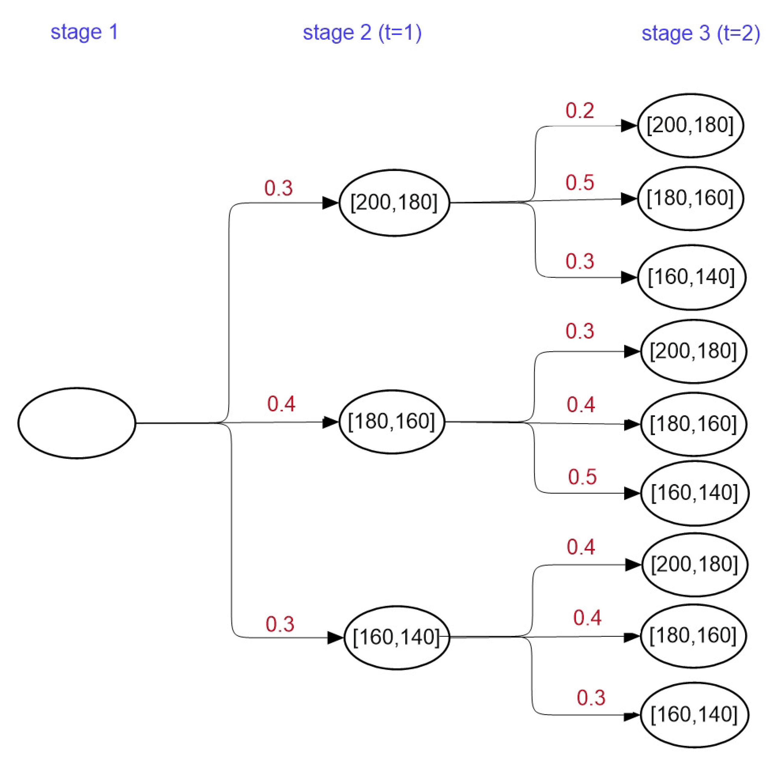
The values for demands can be obtained from the Figure 4. The object function for the KANDW3 Problem [77,78] can be expressed as

$$f(x,v)=min\left(\sum _{i,t}{c}_i{x}_{it}+\mathbb{E}\left[\sum _{j,t}{h}_{jt}{y}_{jt}\right]\right).$$

(13)

$$\begin{array}{ccc}\hfill \mathrm{s}.\mathrm{t}.& \sum _{i,t}{x}_{it}& \le b,\hfill \\ & v\sum _i{a}_{ij}{x}_{it}+y_{jt}& \ge d_{jt},\forall j,t,\hfill \\ \hfill & x_{it},y_{jt}& \ge 0,\forall i,j,t.\hfill \\ \hfill \end{array}$$

(14)

5.2.2. Results of KANDW3 Problem

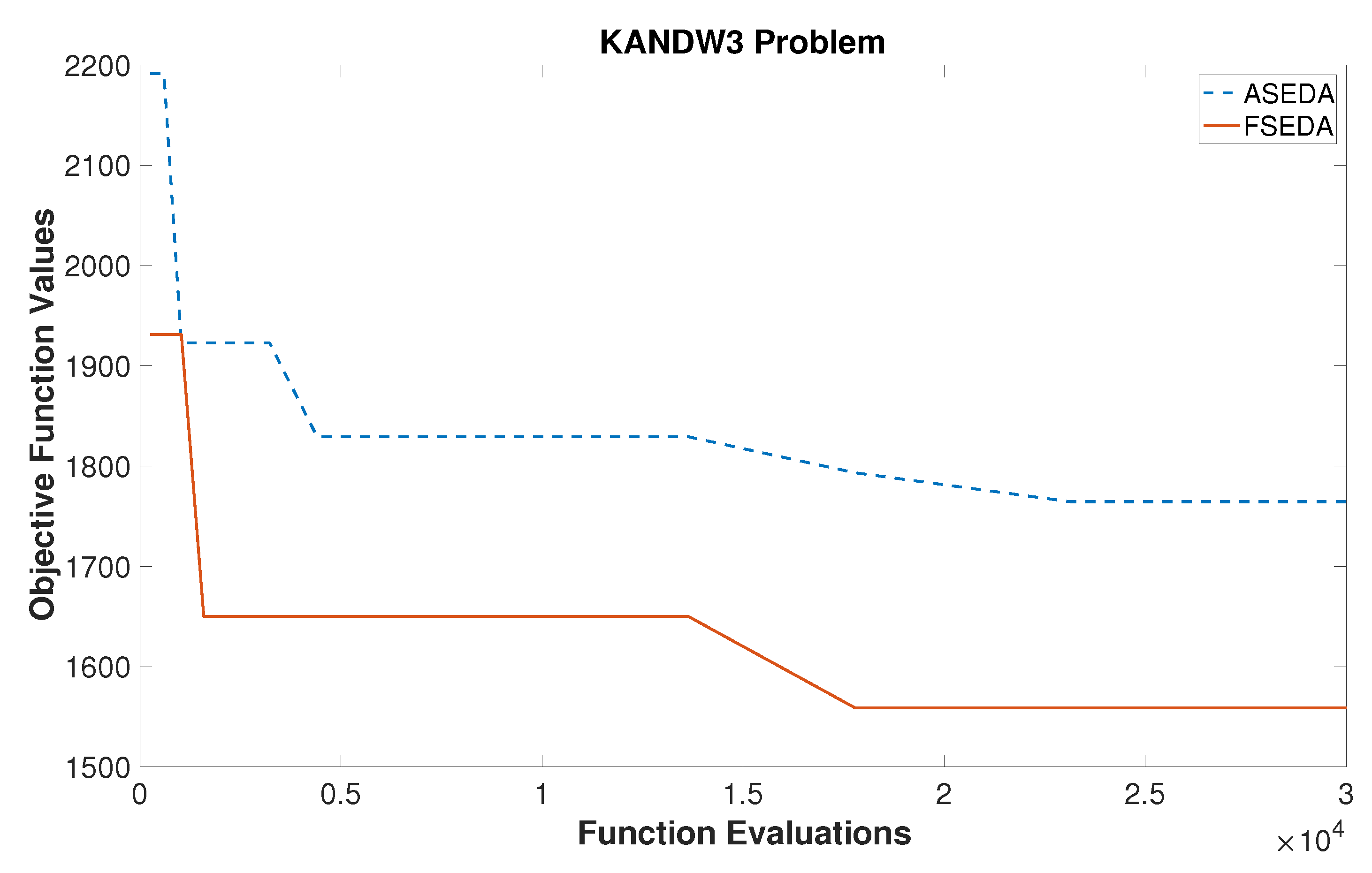
The FSEDA method found the objective function value $f_{min}=1558.9,$ with the decision variable values $x_{min}=(2,13,10,20).$ The best known value for the KANDW3 Problem is $f^{*}=2613$, as mentioned in [78]. Therefore, the proposed method found a new minimal value for the KANDW3 Problem. The comparison between the ASEDA and FSEDA methods is shown in Figure 5. In this figure, the FSEDA method provided better solutions as compared to the ASEDA method.

5.3. The LANDS Problem

Power plants are the key issue in the LANDS Problem [77,79]. Assume that there are four types of power plants which can be operated by three different modes to meet the electricity demands; the operating level $y_{ij}$ of power plant i in mode j to satisfy the demands $d_j$ with the cost $h_{ij}$. The budget b is considered as a constraint which limits the total cost. The main objective is to determine the optimal capacity investment $x_i$ in the power plant i.

5.3.1. The Mathematical Formulation of the LANDS Problem

The formal description of the LANDS Problem can be defined as follows [77,79]. The required values for parameters and constants are also expressed.

i	The power plant type $(i=1,\dots ,4)$.
j	The operating mode $(j=1,\dots ,3).$
$x_i$	The capacity of power plant i (decision variable).
$y_{ij}$	The operating level of power plant i in mode j.
$c_i$	The unit cost of capacity installed for plant type i, $c=[10.0,7.0,16.0,6.0]$.
$h_{ij}$	The unit cost of operating level of power plant i in mode j,
	$h=\left[\begin{array}{ccc}40.0& 24.0& 4.0\\ 45.0& 27.0& 4.5\\ 32.0& 19.2& 3.2\\ 55.0& 33.0& 5.5\end{array}\right]$.
m	The minimum total installed capacity $m=12.0$.
b	The available budget for capacity installment, $b=120.0$.
$d_j$	Random power demands in mode j, $d=[\epsilon ,3.0,2.0],$
	where $\epsilon$ has values 3.0, 5.0, or 7.0 with probability 0.3, 0.4, and 0.3, respectively.

Therefore, the object function for the LANDS Problem [77,79] can be expressed as

$$f(x,v)=min\left(\sum _{i,t}{c}_i{x}_i+\mathbb{E}\left[\sum _{i,j}{h}_{ij}{y}_{ij}\right]\right),$$

(15)

$$\begin{array}{ccc}\hfill \mathrm{s}.\mathrm{t}.& \sum _i{x}_i& \ge m,\hfill \\ \hfill & \sum _i{c}_i{x}_i& \le b,\hfill \\ & \sum _j{y}_{ij}& \le x_i,\forall i,\hfill \\ \hfill & \sum _i{y}_{ij}& \ge {\overline{d}}_j,\forall j,\hfill \\ \hfill & x_i,y_{ij}& \ge 0.\forall i,j.\hfill \\ \hfill \end{array}$$

(16)

5.3.2. Results of the LANDS Problem

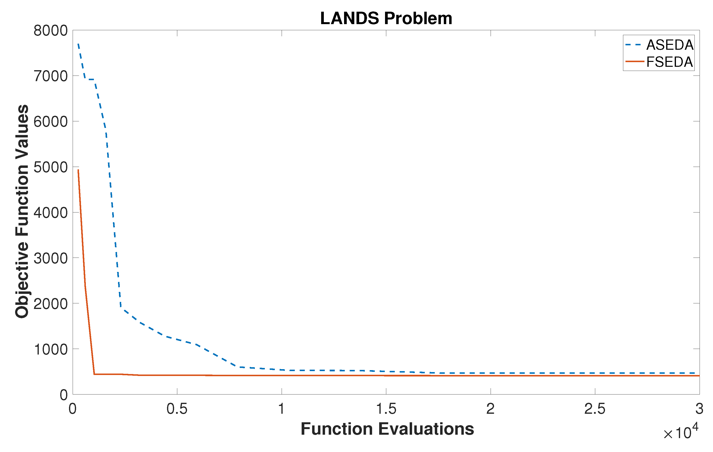
The objective function value $f_{min}=413.616$ was obtained by the FSEDA method with the decision variables $x_{min}=(2.6,2.7,2.6,4.3).$ The best known function value for this problem is $f^{*}=381.85$, which is presented in [79]. Figure 6 presents the comparison between the FSEDA and ASEDA performance for the LANDS Problem. In Figure 6, the FSEDA method reached the best solution faster than the ASEDA method.

6. Conclusions

In this paper, four new algorithms are presented to deal with various problems and applications. The first method is called Fuzzy Sampling Random Search (FSRS), which is a new sampling search technique. The other three methods are EDA-based methods which are denoted by DEDA, ASEDA, and FSEDA. The DEDA method is proposed to deal with deterministic nonlinear programming problems. While the ASEDA and FSEDA methods are designed with average and fuzzy sampling techniques, respectively, to deal with stochastic programming problems. Several sets of benchmark tests involving nonlinear and stochastic programming problems were tested, and the results demonstrate the promising performance of the novel methods. In fact, using a fuzzy membership function is very efficient in containing the anomalous function simulations resulting from small sample sizes. The numerical simulations show that the ASEDA and FSEDA methods are promising simulation-based optimization tools. Moreover, the FSEDA method obtained new optimal solutions for two out of three real-world applications. Finally, the experimental analysis of the proposed methods has enabled us to suggest extending the present work using different metaheuristics to solve simulation-based optimization problems in both continuous and combinatorial domains.

References

1. Kizhakke Kodakkattu, S.; Nair, P. Design optimization of helicopter rotor using kriging. Aircr. Eng. Aerosp. Technol. 2018, 90, 937–945. [Google Scholar] [CrossRef]
2. Kim, P.; Ding, Y. Optimal design of fixture layout in multistation assembly processes. IEEE Trans. Autom. Sci. Eng. 2004, 1, 133–145. [Google Scholar] [CrossRef]
3. Kleijnen, J.P. Simulation-optimization via Kriging and bootstrapping: A survey. J. Simul. 2014, 8, 241–250. [Google Scholar] [CrossRef]
4. Fu, M.C.; Hu, J.Q. Sensitivity analysis for Monte Carlo simulation of option pricing. Probab. Eng. Inf. Sci. 1995, 9, 417–446. [Google Scholar] [CrossRef] [Green Version]
5. Plambeck, E.L.; Fu, B.; Robinson, S.M.; Suri, R. Throughput optimization in tandem production lines via nonsmooth programming. In Proceedings of the 1993 Summer Computer Simulation Conference, Los Angeles, CA, USA, 1 July 1993; pp. 70–75. [Google Scholar]
6. Pourhassan, M.R.; Raissi, S. An integrated simulation-based optimization technique for multi-objective dynamic facility layout problem. J. Ind. Inf. Integr. 2017, 8, 49–58. [Google Scholar] [CrossRef]
7. Semini, M.; Fauske, H.; Strandhagen, J.O. Applications of discrete-event simulation to support manufacturing logistics decision-making: A survey. In Proceedings of the 38th conference on Winter Simulation, Winter Simulation Conference, Monterey, CA, USA, 3–6 December 2006; pp. 1946–1953. [Google Scholar]
8. Chong, L.; Osorio, C. A simulation-based optimization algorithm for dynamic large-scale urban transportation problems. Transp. Sci. 2017, 52, 637–656. [Google Scholar] [CrossRef] [Green Version]
9. Gürkan, G.; Yonca Özge, A.; Robinson, S.M. Sample-path solution of stochastic variational inequalities. Math. Program. 1999, 84, 313–333. [Google Scholar] [CrossRef] [Green Version]
10. Hedar, A.R.; Allam, A.A.; Deabes, W. Memory-Based Evolutionary Algorithms for Nonlinear and Stochastic Programming Problems. Mathematics 2019, 7, 1126. [Google Scholar] [CrossRef] [Green Version]
11. Friedrich, T.; Kötzing, T.; Krejca, M.S.; Sutton, A.M. Robustness of ant colony optimization to noise. Evol. Comput. 2016, 24, 237–254. [Google Scholar] [CrossRef] [Green Version]
12. Ghosh, A.; Das, S.; Mallipeddi, R.; Das, A.K.; Dash, S.S. A modified differential evolution with distance-based selection for continuous optimization in presence of noise. IEEE Access 2017, 5, 26944–26964. [Google Scholar] [CrossRef]
13. Hedar, A.R.; Allam, A.A.; Abdel-Hakim, A.E. Simulation-Based EDAs for Stochastic Programming Problems. Computation 2020, 8, 18. [Google Scholar] [CrossRef] [Green Version]
14. Jin, Y.; Branke, J. Evolutionary optimization in uncertain environments-a survey. IEEE Trans. Evol. Comput. 2005, 9, 303–317. [Google Scholar] [CrossRef] [Green Version]
15. Andradóttir, S. Simulation optimization. In Handbook of Simulation: Principles, Methodology, Advances, Applications, and Practice; John Wiley & Sons: New York, NY, USA, 1998; pp. 307–333. [Google Scholar]
16. Gosavi, A. Simulation-Based Optimization; Springer: Berlin, Germany, 2015. [Google Scholar]
17. Fu, M.C. Optimization for simulation: Theory vs. practice. Inf. J. Comput. 2002, 14, 192–215. [Google Scholar] [CrossRef]
18. BoussaïD, I.; Lepagnot, J.; Siarry, P. A survey on optimization metaheuristics. Inf. Sci. 2013, 237, 82–117. [Google Scholar] [CrossRef]
19. Glover, F.W.; Kochenberger, G.A. Handbook of Metaheuristics; Springer: New York, NY, USA; Philadelphia, PA, USA, 2006; Volume 57. [Google Scholar]
20. Ribeiro, C.C.; Hansen, P. Essays and Surveys in Metaheuristics; Springer Science & Business Media: New York, NY, USA, 2012; Volume 15. [Google Scholar]
21. Siarry, P. Metaheuristics; Springer International Publishing: Cham, Switzerland, 2016. [Google Scholar]
22. Pellerin, R.; Perrier, N.; Berthaut, F. A survey of hybrid metaheuristics for the resource-constrained project scheduling problem. Eur. J. Oper. Res. 2020, 280, 395–416. [Google Scholar] [CrossRef]
23. Doğan, B.; Ölmez, T. A new metaheuristic for numerical function optimization: Vortex Search algorithm. Inf. Sci. 2015, 293, 125–145. [Google Scholar] [CrossRef]
24. Huang, C.; Li, Y.; Yao, X. A Survey of Automatic Parameter Tuning Methods for Metaheuristics. IEEE Trans. Evol. Comput. 2019, 24, 201–216. [Google Scholar] [CrossRef]
25. Larrañaga, P.; Etxeberria, R.; Lozano, J.A.; Peña, J.M. Optimization in continuous domains by learning and simulation of Gaussian networks. In Proceedings of the 2000 Genetic and Evolutionary Computation Conference Workshop Program, Las Vegas, NV, USA, 8–12 July 2000; pp. 201–204. [Google Scholar]
26. Larrañaga, P.; Lozano, J.A. Estimation of Distribution Algorithms: A New Tool for Evolutionary Computation; Springer Science & Business Media: New York, NY, USA, 2001; Volume 2. [Google Scholar]
27. Hauschild, M.; Pelikan, M. An introduction and survey of estimation of distribution algorithms. Swarm Evol. Comput. 2011, 1, 111–128. [Google Scholar] [CrossRef] [Green Version]
28. Yang, Q.; Chen, W.N.; Li, Y.; Chen, C.P.; Xu, X.M.; Zhang, J. Multimodal estimation of distribution algorithms. IEEE Trans. Cybern. 2016, 47, 636–650. [Google Scholar] [CrossRef] [Green Version]
29. Krejca, M.S.; Witt, C. Theory of estimation-of-distribution algorithms. In Theory of Evolutionary Computation; Springer International Publishing: Cham, Switzerland, 2020; pp. 405–442. [Google Scholar]
30. Homem-De-Mello, T. Variable-sample methods for stochastic optimization. ACM Trans. Model. Comput. Simul. (TOMACS) 2003, 13, 108–133. [Google Scholar] [CrossRef]
31. Rakshit, P.; Konar, A. Differential evolution for noisy multiobjective optimization. Artif. Intell. 2015, 227, 165–189. [Google Scholar] [CrossRef]
32. Rakshit, P.; Konar, A.; Das, S. Noisy evolutionary optimization algorithms—A comprehensive survey. Swarm Evol. Comput. 2017, 33, 18–45. [Google Scholar] [CrossRef]
33. Rakshit, P.; Konar, A. Principles in Noisy Optimization; Springer: Berlin, Germany, 2018. [Google Scholar]
34. Zadeh, L.A. Fuzzy sets. Inf. Control 1965, 8, 338–353. [Google Scholar] [CrossRef] [Green Version]
35. Stoyan, D.; Kruse, R. KD Meyer: Statistics with Vague Data. D. Reidel Publishing Company, Dortrecht-Boston-Lancaster-Tokyo 1987, 279 S., Dfl. 150.–; US-$59.–; UK£ 42.–, ISBN 7027725624. Biom. J. 1989, 31, 312. [Google Scholar] [CrossRef]
36. Puri, M.L.; Ralescu, D.A.; Zadeh, L. Fuzzy random variables. In Readings in Fuzzy Sets for Intelligent Systems; Morgan Kaufmann: San Mateo, CA, USA, 1993; pp. 265–271. [Google Scholar]
37. Gil, M.A.; López-Díaz, M.; Ralescu, D.A. Overview on the development of fuzzy random variables. Fuzzy Sets Syst. 2006, 157, 2546–2557. [Google Scholar] [CrossRef]
38. Biswal, M.; Acharya, S. Solving multi-choice linear programming problems by interpolating polynomials. Math. Comput. Model. 2011, 54, 1405–1412. [Google Scholar] [CrossRef]
39. Wang, S.; Watada, J. Fuzzy Stochastic Optimization: Theory, Models and Applications; Springer Science & Business Media: New York, NY, USA, 2012. [Google Scholar]
40. Mousavi, S.M.; Jolai, F.; Tavakkoli-Moghaddam, R. A fuzzy stochastic multi-attribute group decision-making approach for selection problems. Group Decis. Negot. 2013, 22, 207–233. [Google Scholar] [CrossRef]
41. Acharya, S.; Ranarahu, N.; Dash, J.K.; Acharya, M.M. Computation of a multi-objective fuzzy stochastic transportation problem. Int. J. Fuzzy Comput. Model. 2014, 1, 212–233. [Google Scholar] [CrossRef]
42. Lacagnina, V.; Pecorella, A. A stochastic soft constraints fuzzy model for a portfolio selection problem. Fuzzy Sets Syst. 2006, 157, 1317–1327. [Google Scholar] [CrossRef]
43. Dong, W.; Chen, T.; Tiňo, P.; Yao, X. Scaling up estimation of distribution algorithms for continuous optimization. IEEE Trans. Evol. Comput. 2013, 17, 797–822. [Google Scholar] [CrossRef] [Green Version]
44. Mühlenbein, H.; Paass, G. From recombination of genes to the estimation of distributions I. Binary parameters. In International Conference on Parallel Problem Solving From Nature; Springer: Berlin, Germany, 1996; pp. 178–187. [Google Scholar]
45. Sebag, M.; Ducoulombier, A. Extending population-based incremental learning to continuous search spaces. In International Conference on Parallel Problem Solving from Nature; Springer: Berlin, Germany, 1998; pp. 418–427. [Google Scholar]
46. Bosman, P.A.; Thierens, D. Expanding from Discrete to Continuous Estimation of Distribution Algorithms: The ID𝔼A. In International Conference on Parallel Problem Solving from Nature; Springer: Berlin, Germany, 2000; pp. 767–776. [Google Scholar]
47. Bosman, P.A.; Thierens, D. Continuous iterated density estimation evolutionary algorithms within the IDEA framework. In Proceedings of the 2000 Genetic and Evolutionary Computation Conference Workshop Program, Las Vegas, NV, USA, 8–12 July 2000; pp. 197–200. [Google Scholar]
48. Wagner, M.; Auger, A.; Schoenauer, M. EEDA: A New Robust Estimation of Distribution Algorithms; Research Report (RR-5190); INRIA: Rocquencourt, France, 2004; No. inria-00070802; p. 16. [Google Scholar]
49. Grahl, J.; Bosman, P.A.; Rothlauf, F. The correlation-triggered adaptive variance scaling IDEA. In Proceedings of the 8th Annual Conference on Genetic and Evolutionary Computation, Seattle, WA, USA, 8–12 July 2006; pp. 397–404. [Google Scholar]
50. Bosman, P.A.; Grahl, J.; Rothlauf, F. SDR: A better trigger for adaptive variance scaling in normal EDAs. In Proceedings of the 9th Annual Conference on Genetic and Evolutionary Computation, London, UK, 25–28 September 2007; pp. 492–499. [Google Scholar]
51. Dong, W.; Yao, X. Unified eigen analysis on multivariate Gaussian based estimation of distribution algorithms. Inf. Sci. 2008, 178, 3000–3023. [Google Scholar] [CrossRef] [Green Version]
52. Yuan, B.; Gallagher, M. Playing in continuous spaces: Some analysis and extension of population-based incremental learning. In Proceedings of the 2003 Congress on Evolutionary Computation, Canberra, Australia, 8–12 December 2003; Volume 1, pp. 443–450. [Google Scholar]
53. Pošík, P. Distribution tree-building real-valued evolutionary algorithm. In International Conference on Parallel Problem Solving from Nature; Springer: Berlin, Germany, 2004; pp. 372–381. [Google Scholar]
54. Ding, N.; Zhou, S.; Sun, Z. Optimizing continuous problems using estimation of distribution algorithm based on histogram model. In Asia-Pacific Conference on Simulated Evolution and Learning; Springer: Berlin, Germany, 2006; pp. 545–552. [Google Scholar]
55. Ding, N.; Xu, J.; Zhou, S.; Sun, Z. Reducing computational complexity of estimating multivariate histogram-based probabilistic model. In Proceedings of the 2007 IEEE Congress on Evolutionary Computation, Singapore, 25–28 September 2007; pp. 111–118. [Google Scholar]
56. Ding, N.; Zhou, S. Linkages detection in histogram-based estimation of distribution algorithm. In Linkage in Evolutionary Computation; Springer: Berlin, Germany, 2008; pp. 25–40. [Google Scholar]
57. Ding, N.; Zhou, S.D.; Sun, Z.Q. Histogram-based estimation of distribution algorithm: A competent method for continuous optimization. J. Comput. Sci. Technol. 2008, 23, 35–43. [Google Scholar] [CrossRef]
58. Ding, N.; Zhou, S.; Zhang, H.; Sun, Z. Marginal probability distribution estimation in characteristic space of covariance-matrix. In Proceedings of the 2008 IEEE Congress on Evolutionary Computation (IEEE World Congress on Computational Intelligence), Hong Kong, China, 1–6 June 2008; pp. 1589–1595. [Google Scholar]
59. Bosman, P.A.; Thierens, D. Numerical optimization with real-valued estimation-of-distribution algorithms. In Scalable Optimization via Probabilistic Modeling; Springer: Berlin, Germany, 2006; pp. 91–120. [Google Scholar]
60. Wang, X.; Kerre, E. On the classification and the dependencies of the ordering methods. In Fuzzy Logic Foundations and Industrial Applications; Springer: Berlin, Germany, 1996; pp. 73–90. [Google Scholar]
61. Klir, G.; Yuan, B. Fuzzy Sets and Fuzzy Logic; Prentice Hall: Upper Saddle River, NJ, USA, 1995; Volume 4. [Google Scholar]
62. Hedar, A.R.; Fukushima, M. Tabu search directed by direct search methods for nonlinear global optimization. Eur. J. Oper. Res. 2006, 170, 329–349. [Google Scholar] [CrossRef] [Green Version]
63. García, S.; Fernández, A.; Luengo, J.; Herrera, F. A study of statistical techniques and performance measures for genetics-based machine learning: Accuracy and interpretability. Soft Comput. 2009, 13, 959. [Google Scholar] [CrossRef]
64. Sheskin, D.J. Handbook of Parametric and Nonparametric Statistical Procedures; CRC Press: Boca Raton, FL, USA, 2003. [Google Scholar]
65. Zar, J.H. Biostatistical Analysis, 5th ed.; Pearson: Upper Saddle River, NJ, USA, 2013. [Google Scholar]
66. Derrac, J.; García, S.; Molina, D.; Herrera, F. A practical tutorial on the use of nonparametric statistical tests as a methodology for comparing evolutionary and swarm intelligence algorithms. Swarm Evol. Comput. 2011, 1, 3–18. [Google Scholar] [CrossRef]
67. García-Martínez, S.; Molina, D.; Lozano, M.; Herrera, F. A study on the use of non-parametric tests for analyzing the evolutionary algorithms’ behaviour: A case study on the CEC’2005 special session on real parameter optimization. J. Heuristics 2009, 15, 617–644. [Google Scholar] [CrossRef]
68. Hedar, A.R.; Allam, A.A. Scatter Search for Simulation-Based Optimization. In Proceedings of the 2017 International Conference on Computer and Applications (ICCA), Doha, UAE, 6–7 September 2017; pp. 244–251. [Google Scholar]
69. Brest, J.; Greiner, S.; Boskovic, B.; Mernik, M.; Zumer, V. Self-adapting control parameters in differential evolution: A comparative study on numerical benchmark problems. IEEE Trans. Evol. Comput. 2006, 10, 646–657. [Google Scholar] [CrossRef]
70. Aizawa, A.N.; Wah, B.W. Scheduling of genetic algorithms in a noisy environment. Evol. Comput. 1994, 2, 97–122. [Google Scholar] [CrossRef]
71. Das, S.; Konar, A.; Chakraborty, U.K. Improved differential evolution algorithms for handling noisy optimization problems. In Proceedings of the 2005 IEEE Congress on Evolutionary Computation, Edinburgh, UK, 2–5 September 2005; Volume 2, pp. 1691–1698. [Google Scholar]
72. Rahnamayan, S.; Tizhoosh, H.R.; Salama, M.M. Opposition-based differential evolution algorithms. In Proceedings of the 2006 IEEE International Conference on Evolutionary Computation, Vancouver, BC, Canada, 16–21 July 2006; pp. 2010–2017. [Google Scholar]
73. Caponio, A.; Neri, F. Differential evolution with noise analyzer. In Workshops on Applications of Evolutionary Computation; Springer: Berlin, Germany, 2009; pp. 715–724. [Google Scholar]
74. Mininno, E.; Neri, F. A memetic differential evolution approach in noisy optimization. Memetic Comput. 2010, 2, 111–135. [Google Scholar] [CrossRef]
75. Ghosh, A.; Das, S.; Panigrahi, B.K.; Das, A.K. A noise resilient differential evolution with improved parameter and strategy control. In Proceedings of the 2017 IEEE Congress on Evolutionary Computation (CEC), San Sebastian, Spain, 5–8 June 2017; pp. 2590–2597. [Google Scholar]
76. King, A. Stochastic programming problems: Examples from the literature. Numer. Tech. Stoch. Optim. 1988, 3, 543–567. [Google Scholar]
77. King, A.J.; Wright, S.E.; Parija, G.R.; Entriken, R. The IBM stochastic programming system. In Applications of Stochastic Programming; SIAM: Philadelphia, PA, USA, 2005; pp. 21–36. [Google Scholar]
78. Kall, P.; Wallace, S. Stochastic Programming; John Wiley & Sons: Chichester, UK, 1994. [Google Scholar]
79. Louveaux, F.V. Optimal Investments for Electricity Generateion: A Stochastic Model and A Test Problem. In Numerical Techniques for Stochastic Optimization; Springer: Berlin, Germany, 1988; Volume 10, pp. 445–454. [Google Scholar]
80. Smith, A.E.; Coit, D.W. Penalty functions. Handb. Evol. Comput. Pages C 1997, 5, 1–6. [Google Scholar]
Figure 1. Average errors using different settings of parameter R for simulation-based optimization problems using Test Set C.
Applsci 10 06937 g001
Figure 2. The performance of Fuzzy Sampling Random Search (FSRS) and SPRA with different sample sizes.
Applsci 10 06937 g002
Figure 3. The FSEDA and ASEDA performance for the product mix (PROD-MIX) Problem.
Applsci 10 06937 g003
Figure 4. Demand values in the The modified production planning Kall and Wallace (KANDW3) Problem.
Applsci 10 06937 g004
Figure 5. The FSEDA and ASEDA performance for the KANDW3 Problem.
Applsci 10 06937 g005
Figure 6. The FSEDA and ASEDA performance for the two-stage optimal capacity investment Louveaux and Smeers (LANDS) Problem.
Applsci 10 06937 g006