Comparison and Ranking of Metaheuristic Techniques for Optimization of PI Controllers in a Machine Drive System

Abstract

Proportional integral (PI) control is still the most widely deployed controller in the industrial drives due to its simplicity and the fact that it is easy to understand and implement. Nevertheless, they are successes applied to systems with a complex behavior with a nonlinear representation, but a disadvantage is the procedure to find the optimal PI controller gains. The optimal values of PI parameters must be computed during the tuning process. However, traditional tuning techniques are based on model and do not provide optimal adjustment parameters for the PI controllers because the transient response could produce oscillations and a large overshoot. In this paper, six swarm intelligence-based algorithms (whale, moth-flame, flower pollination, dragonfly, cuckoo search, and modified flower pollination), are correctly conditioned and delimited to tune the PI controllers, the results are probed in a typical industry actuator. Also, a rigorous study is developed to evaluate the quality and reliability of these algorithms by a statistical analysis based on non-parametric test and post-hoc test. Finally, with the obtained results, some time simulations are carried out to corroborate that the nonlinear system performance is improved for high precision industrial applications subjected to endogenous and exogenous uncertainties in a wide range of operating conditions.

1. Introduction

Alternating current (AC) motors are widely used in industrial applications such as electric vehicles, hybrid electric vehicle, wind generation systems, mining machinery, marine propulsion, industrial robots, air conditioners, cranes, among other applications, as well as particular demand in residential and commercial areas [1,2]. There are two main categories of AC motors: induction motors (IM) and synchronous motors (SM), the last one, are gaining great attention due to its self-excitation, high efficiency, low maintenance cost, high power density, fast dynamic response, high torque-to-inertia, and more economic maintenance compared to direct current and induction machines. [3,4].

During recent decades, the permanent magnet synchronous motor (PMSM) has been used more and more due to its advantages; but at the same time, too many control structures have been developed to enhance the performance due to the nonlinears, and endogenous and exogenous disturbances [5]. Some of them include classical controllers, intelligent control, vector control, backstepping technique, linear quadratic regulator, fuzzy logic controller, artificial neural networks, genetic algorithm, predictive control, and robust control [6]. Vector control with classical controllers, Figure 1, is the most widely used controller in industries due its easy design and implementation procedure. Moreover, in the literature, proportional integral derivative (PID) controllers have been extensively studied to prove stability of PMSM dynamic performance and improve its operation under critical scenarios [7,8]. In [9] shows that the PMSM is globally regulated around a desired equilibrium point, with a simple PI control around current errors, if the gains are suitably chosen. Therefore, a control scheme based on traditional PI controllers is a proper choice for velocity trajectory tracking.

The advantages of a PID controller are its feasibility, simplicity, ease to understand, and implementation stage. However, a disadvantage of the traditional PID controller is the procedure to find the optimal PID gains for a particular system that is very difficult and tedious to perform [10,11,12,13]. In the literature, there are several techniques to solve the problem of gains tuning of conventional PID and PI controllers when the system is non-linear, such as the PMSM. Traditional tuning techniques do not provide optimal adjustment parameters for the PID controllers because the transient response could produce oscillations and a large overshoot due to the system dynamics [14]. Therefore, new regulation strategies know as advanced and intelligent schemes have been applied to overcome the main drawbacks of PID controller in tuning stage, by the solution of an objective function to achieve optimal gains.

A crucial problem in nonlinear systems control design and PID scheme is the definition of a set of controller gains that provide a system performance near-optimal. This process, which is usually carried out at the design stage as a compensation regarding various adverse factors, often produces restricted results. Thus, algorithms inspired in nature and population seems like an important alternative to synergistically operate with PID controller for improving the system behavior [10].

In recent literature, various metaheuristic algorithms have been used to carry out an inclusive search for optimal solutions, which cannot be solved by classical techniques. That the metaheuristic algorithms try to emulate the natural behavior of different class of animals, outcomes to have a high level of efficiency, overcome limitations of classical methodologies. Besides, search results depend on the system complexity or the problem to solve; becouse a metaheuristic algorithm can be more efficient than other to solve a particular problem, while the same metaheuristic algorithm could present a poor performance for another system [15].

In this context, different optimization techniques, such as cuckoo search algorithm (CSA) [14], biogeography-based optimization (BBO) [16], firefly algorithm (FA) [17], hybrid FA-pattern search [18], krill herd algorithm [19], flower pollination algorithm (FPA) [12], hybrid flower pollination algorithm (HFPA) [20], grey wolf optimization algorithm (GWO) [21], bacterial foraging algorithm [22], particle swarm optimization (PSO) [23], differential evolution [24], artificial bee colony (ABC) [25], whale optimization algorithm (WOA) [26], moth-flame optimization algorithm (MOA) [27], dragonfly algorithm (DA) [13] have been developed and can be used to compute the optimal PID controller gains of many dynamic systems. However, useful algorithms’ performance depends on the adequate search procedure, which implies the correct objective function definition, search limits, the setting the search algorithm control parameters, and the complexity of the analysis system.

In [28] a WOA application is presented to optimally design PID controllers in the automatic generation control loops of interconnected power systems, including renewable energy sources. The effectiveness of the proposed controller to deal with the uncertainties in generation systems is an essential feature of this study.

An objective function to enhance transient response of terminal voltage in terms of maximum overshoot, rise time, settling time, and steady state error is solved by CSA algorithm [14]. A PID controller is used in automatic voltage regulator scheme. Also, in [10] the automatic control problem of synchronous generator is attended with MOA optimization procedure.

In [13] DA, is applied for design and implementation of a PID controller with three degrees of freedom. The control stabilizes the frequency and power fluctuations after some disturbance is presented in a hybrid topology of an electric distribution system.

In [29] a meta-heuristic optimization algorithm called chaotic whale optimization algorithm is used to regulate the performance of PMSM when it is affected by load disturbances and changes in system parameters. In [30] a control system for permanent magnet synchronous motors, together with an online self-tuning method is presented. In this work, a meta-heuristic bio-inspired approach has been implemented to find the voltage source converter parameter set which minimizes a specific objective function. In the last three cases, there is not a robustness analysis, sensitivity analysis, or statistical test to affirm robust performance of designed controller, analyze the effectiveness of the controller and verify the significance of the results, respectively.

The purpose of this paper is to compare different reactive, nature-inspired algorithms for tuning parameters of the PID controller in order to discover the most suitable algorithm for use in solving this class of problem. The six nature-inspired algorithms such as whale, moth-flame, flower pollination, dragonfly, cuckoo search, and modified flower pollination are compared in order to show which of them are the best to work with the same population sizes and generation numbers. This proposal uses six nature-inspired algorithms to search optimal values of a regulatory scheme for robust tracking tasks of desired velocity profiles of a PMSM [31]. This evolutionary technique is applied on one objective/fitness function to find an optimal solution that minimizes the overall error.

In another context, the contributions of a meta-heuristic must be objectively evaluated and reported; however, as described in [32], this is not always the case. This is due to the fact that the meta-heuristic procedures are not described in sufficient detail, the experimental adjustments are very generally described and this results in the impossibility of replicating an experiment exactly and an equitable comparison as mentioned in [33]. Statistical analysis [34] is used for the objective evaluation of the performance of metaheuristic algorithms. The statistical procedures developed to carry out statistical analyzes can be classified into two: parametric and non-parametric, according to the specific type of data used [35]. In many experimental studies, the lack of properties required for proper application of parametric procedures (independence, normality, and homoscedasticity) gives non-parametrics the task of rigorous comparison between algorithms. Due to the above, the use of non-parametric statistical analysis is widely used in the field of metaheuristics [34] to establish its performance.

Due to different current drawbacks in PMSM regulation, some objectives could be included in the controller design stage: (a) Search simultaneously optimum values of a regulation scheme for robust tracking tasks of desired velocity profiles of a PMSM using six nature-inspired algorithms. To explore optimum controller settings, an extensive comparative study is carried out with different performance index and time domain specification; (b) in order to investigate the effectiveness of the velocity trajectory tracking controller tuned with six nature-inspired algorithms, the comparison of the transient response of the PMSM subject to different operating conditions is made; (c) to examine the robustness of the velocity trajectory tracking controller tuned with six nature-inspired algorithms, a sensitivity analysis under parametric variation and different operating conditions of the PMSM is done; and (d) The presented results exhibit high quality behavior and is demonstrated by a statistical analysis based on non parametric test and post hoc test.

The remainder of the paper is organized as follows. Section 2 portrays the mathematical model of a nonlinear PMSM. The control structure is presented in Section 3. The objective function and constraints for the optimization of PI gains are described in Section 4. An overview of the six nature-inspired algorithms are presented in Section 5. In Section 6 presents optimization results, sensitivity analysis and robustness of controller. Section 6 shows the statistical analysis for comparing nature-inspired optimization algorithms. Finally, the conclusions of the paper are established.

2. Analytical Representation Regulation Scheme of PMSM

2.1. Dynamic Model

The set of nonlinear differential equations that describe the dynamics of a three-phase PMSM drive in the $dq$ reference frame oriented to the rotor flux axis can be written as [36]:    

$$\frac{d{i}_d}{dt}=(-R_s{i}_d+{\omega }_e{L}_q{i}_q-v_d)\left(\frac{1}{L_d}\right)$$

(1)

$$\frac{d{i}_q}{dt}=(-R_s{i}_q+{\omega }_e{L}_d{i}_d-{\omega }_e{\lambda }_m-v_q)\left(\frac{1}{L_q}\right)$$

(2)

$$\frac{d{\omega }_r}{dt}=\frac{0.75P{i}_q({\lambda }_m+(L_d-L_q)i_d)-T_l-B{\omega }_r}{J}$$

(3)

$$\frac{d{\theta }_r}{dt}={\omega }_r$$

(4)

where $R_s$ is the stator winding resistance per-phase; ${\omega }_e$ is the electrical rotor angular speed; $L_d$ and $L_q$ are the stator winding self-inductances in the d and q axes, respectively; $i_q$ is the q-axis stator current; $v_q$ is the q-axis stator voltage; $i_d$ is the d-axis stator current; $v_d$ is the d-axis stator voltage; ${\lambda }_m$ is the magnetic flux linkage in the rotor due to the magnets; J and B are the inertia moment and the viscous friction coeffcient, respectively; $T_l$ is the disturbance signal; P is the number of pole pairs; ${\theta }_r$ and ${\omega }_r$ are position and the mechanical speed of the rotor (${\omega }_e$ = P${\omega }_r$), respectively.

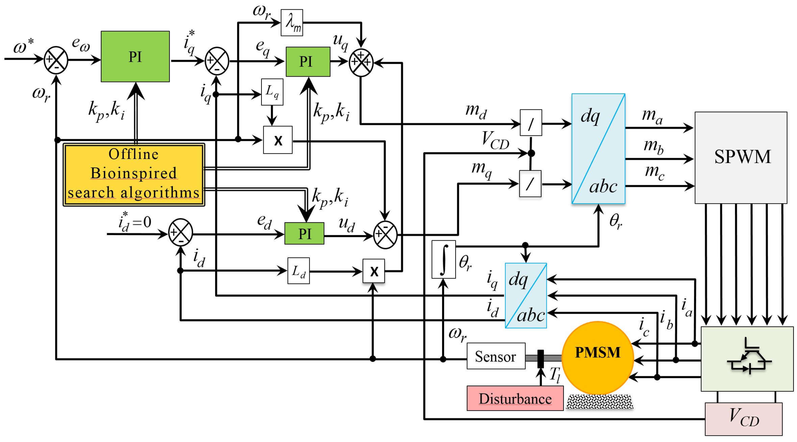
2.2. Control Algorithm

The system depicted in (1)–(4) is a set of coupled nonlinear differential equations with two control inputs, $v_d$ and $v_q$ and one disturbance signal ($T_l$). The main task of the PMSM drive based on linear controllers is to design an asymptotically stable regulation scheme for robust tracking tasks against different operating conditions and desired speed reference profiles.

The PMSM used in this servo system demands a particular configuration of control scheme, Figure 1. The system contains a permanent magnet synchronous motor, a field oriented control, coordinate transformations $abc$ to $dq$ and vice versa, a sinusoidal pulse width modulation, a power source rectifier based on semiconductor devices, a direct current voltage bus ($V_{CD}$) an encoder used to detect speed and three PI controllers. The controllers apply a structure of cascade control loops, consisting of an external speed loop and two inners currents loops. The cascade control is used to attenuate the effect of disturbances. In this work, the three control loops are used to track desired speed reference profiles and provide robustness against exogenous disturbances (mechanical load torque) and parametric variations due to operating temperature.

The external control loop with negative feedback is used for speed regulation and compensate variations of load torque. Figure 1 shows that the outer control loop computes the desired current signal $\left(i_q^{\ast }\right)$ in q axes, for the desired speed ${\omega }^{\ast }$ with the rotor speed error signal $e_{\omega }$. The expression to compute the rotor speed error signal can be represented as,

$$e_{\omega }={\omega }^{\ast }-{\omega }_r$$

(5)

where ${\omega }^{\ast }$ is the desired rotor speed and $e_{\omega }$ is the rotor speed error. The external loop equation can be expressed as

$$\begin{array}{c}\hfill i_q^{\ast }=k_{p,{\omega }_r}({\omega }^{\ast }-{\omega }_r)+k_{i,{\omega }_r}{\int }_0^t({\omega }^{\ast }\left(\tau \right)-{\omega }_r\left(\tau \right))d\tau \end{array}$$

(6)

where $k_{p,{\omega }_r}$ and $k_{i,{\omega }_r}$ are the proportional gain of rotor speed and the integral gain of rotor speed, respectively. The two internal control loops are called the secondary control. The inner loops attenuate the effect due to the parametric variations of PMSM. The equations of the two internal control loops are given by

$$\begin{array}{c}\hfill v_d=k_{p,i_d}(i_d^{\ast }-i_d)+k_{i,i_d}{\int }_0^t(i_d^{\ast }\left(\tau \right)-i_d\left(\tau \right))d\tau -L_q{\omega }_e{i}_q\\ \hfill v_q=k_{p,i_q}(i_q^{\ast }-i_q)+k_{i,i_q}{\int }_0^t(i_q^{\ast }\left(\tau \right)-i_q\left(\tau \right))d\tau +L_d{\omega }_e{i}_d+{\omega }_e{\lambda }_m\end{array}$$

(7)

where $k_{p,i_d}$ and $k_{i,i_d}$ are proportional and integral gains of the current on d-axis, respectively; $i_d^{\ast }$ is the d-axis current reference value, $k_{p,i_q}$ and $k_{i,i_q}$ are proportional and integral gains of the current on q-axis, respectively; and

$$\begin{array}{c}\hfill v_d=L_q{\omega }_e{i}_q+U_d\\ \hfill v_q=-L_d{\omega }_e{i}_d-{\omega }_e{\lambda }_m+U_q\end{array}$$

(8)

where $U_d$ and $U_q$ are two new auxiliary control variables. The auxiliary variables are used to obtain the desired dynamics for the PMSM stator currents eliminating the nonlinearities and the coupling of the mechanical and electrical variables indicated in (1) and (2) [7,37]. Thus, $k_{p,i_q}$, $k_{i,i_q}$, $k_{p,i_d}$, $k_{i,i_d}$, $k_{p,{\omega }_r}$ and $k_{i,{\omega }_r}$ are computed simultaneously using six nature-inspired algorithms to ensure high speeds tracking performance and efficient disturbances rejection. The purpose of this analysis is to compare different reactive, nature-inspired algorithms for tuning parameters of the PID controller in order to discover the most suitable algorithm for the velocity trajectory tracking controller problem.

3. Objective Function for Parameters Tuning

The objective function to compute the gains of the controllers can be designed in different ways. In previous works, the objective function is constructed by one or more performance indices, such as: integral squared error (JISE), integral absolute error (JIAE), integral time and squared error (JITSE), mean squared error (MSE) and integral of time and absolute error (JITAE). Nevertheless, some researchers have been used different fitness functions based on time domain specifications response, such as: settling time ($t_s$), rise time ($t_r$), maximum overshoot ($M_p$) and steady state error ($e_{ss}$). In this paper, to design the objective function, both criteria of transient response and performance indices are used in order to minimize all the indices as mentioned earlier. [14,38,39]. Thus, the respective objective function is defined as [40],

$$\begin{array}{cc}\hfill & minJ=(1-ex{p}^{-\gamma })(M_p+e_{ss})+ex{p}^{-\gamma }(t_s-t_r)\hfill \end{array}$$

(9)

subject to the following constraints:

$$\begin{array}{cc}\hfill & k_{p,j}^{min}\le k_p\le k_{p,j}^{max}\hfill \\ \hfill & k_{i,j}^{min}\le k_i\le k_{i,j}^{max}\hfill \end{array}$$

(10)

where $j=[i_q,i_d,{\omega }_r]$; $k_{p,j}^{min}$, $k_{i,j}^{min}$, $k_{p,j}^{max}$ and $k_{i,j}^{max}$ are the maximum and minimum values of the gains of the PI controllers, and $\gamma$ is the weighting factor which could be changed according to the dynamics of the system, in this work $\gamma$ = 0.5. The search space for proportional gains $\left(k_{p,j}\right)$ are defined between 0.1 and 100; and that of the integral gains $\left(k_{i,j}\right)$ are between 0.1 and 250.

4. Description of Search Algorithms

4.1. Overview of Cuckoo Search Optimization

The CSA is an algorithm based on the aggressive strategy of reproduction of the cuckoo birds and the characteristics of flights called Lévy of some species of birds [41]. CSA starts when the mother cuckoo lays her eggs in alien nests. The host bird can discover that the eggs are not its own and either destroy the eggs or leave the nest with all the eggs inside. CSA starts with an initial population randomly distributed to search for a nest to lay the egg. The random position of the nest where the egg is placed is decided by carrying out Levy flights, defined as:

$$x(t+1)=x\left(t\right)+\alpha \otimes \mathrm{Lévy}\left(\lambda \right)$$

(11)

where t is the current generation number and $\alpha >0$ is the step size. The product ⊗ means entry-wise multiplication. Basically, Lévy flights provide a random walk, while their random steps are extracted from a Lévy distribution, which for large steps has an infinite variance with an infinite average, with the form

$$\mathrm{Lévy}\sim u=t^{(-\lambda )},(-1<\lambda \le 3)$$

(12)

In the real world, if the egg of a cuckoo bird is very similar to the egg of the nest-owning bird, then the egg has less chance of being discovered so the suitability must be related to the difference in solutions. Following the rules defined above, the optimization algorithm can be summarized in Algorithm 1.

Algorithm 1: Cuckoo Search Optimization

begin       Objective function J, $k_{i,j}$ = [$k_{p,i_d}$, $k_{i,i_d}$, $k_{p,i_q}$, $k_{i,i_q}$, $k_{p,e_{\omega }}$,$k_{i,e_{\omega }}$]       Generate initial population of $\mathbf{N}$ host nests $x_i$ $(i=1,2,\dots ,N)$       while ($t<$ Max Generation) or (stop criterion)             Get a cuckoo randomly by Lévy flights             Evaluate its fitness             Choose a nest among N randomly             if $(F_i>F_j)$                   Replace j by the new solution             end if             Abandon a fraction ($p_a$) of worse nests             Keep the best solutions (or nests with quality solutions)             Rank the solutions and find the current best       end while       Show results and visualization end

4.2. Overview of Dragonfly Algorith

The dragonfly, is one of the most interesting and fascinating insects of nature. Currently, more than 5500 different species of dragonflies are known. Dragonfly Algorithm mimicks the swarming behaviours of a dragonfly. The inspiration of the DA [42] is taken from the social behavior of the dragonflies to hunt their food (static swarm) and when they migrate (dynamic swarm). Considering these two behaviors, there are five factors involved in determining the individual dragonfly position: (a) Separation; (b) Alignment motion; (c) Cohesion motion; (d) Food Attraction; and (e) Predator distraction. There are two ways for updating the individual dragonfly position depending on the neighborhood position. If there is no dragonfly in the neighborhood radius, the individual position is updated considering the Levy flight equation and given as follow:

$$X_{t+1}=X_t+\mathrm{lévy}\left(d\right)X_t$$

(13)

where d is the number of decision variables. The Lévy flight function is given by

$$\mathrm{lévy}\left(d\right)=0.01\frac{r_1\rho }{{\left|r_2\right|}^{1/\beta }}$$

(14)

where $r_1$ and $r_2$ are two random numbers in [0, 1]; $\beta$ is a constant and $\rho$ is computed as

$$\rho ={\left(\frac{\Gamma \left(1+\beta \right)sin\left(\frac{\pi \beta }{2}\right)}{\Gamma \left(\frac{1+\beta }{2}\right)\beta 2^{\left(\frac{\beta -1}{2}\right)}}\right)}^{\frac{1}{\beta }}$$

(15)

where $\Gamma \left(x\right)=\left(x-1\right)!$. Otherwise, the new position is calculated as follow:

$$X_{t+1}=X_t+\mathsf{\Delta }{X}_{t+1}$$

(16)

where $\mathsf{\Delta }{X}_{t+1}$ is the step vector and can be obtained as

$$\mathsf{\Delta }{X}_{t+1}=(s{S}_i+a{A}_i+c{C}_i+f{F}_i+e{E}_i)+w\mathsf{\Delta }{X}_t$$

(17)

where s shows the separation weight; a is the alignment weight; c is the cohesion weight; f is a food factor; e is the enemy factor; w is the inertia weight, $S_i$ indicates the separation of the $i\text{-th}$ individual, $A_i$ is the alignment of $i\text{-th}$ individual, $C_i$ is the cohesion of the $i\text{-th}$ individual, $F_i$ is the food source of the $i\text{-th}$ individual, $E_i$ is the position of enemy of the $i\text{-th}$ individual and t is the iteration number. The optimization process of DA is further explained in Algorithm 2:

Algorithm 2: Dragonfly Algorithm

Define population size (M)       Begin the iteration counter $t=1$       Initialize the population by generating $X_i$ for $i=1,2,3\dots ,M$       Calculate the objective function values of all dragonflies       Update the food and the predator’s location       While (the stop criterion is not satisfied) do             For $i=1:M$                   Update neighborhood radius (or update $w,s,a,c,f$, and e)                   If a dragonfly has at least one neighborhood dragonfly                         Separation motion                         Alignment motion                         Cohesion motion                         Food attraction motion                         Predator distraction motion                   Else                         Update position vector using the Lévy flight function                   End if             End for i             Sort the population/dragonflies from best to and find the current best       End while

4.3. Overview of Flower Pollination Algorithm

FPA was developed by Xin-She Yang in 2012 [43] and is considered to be an excellent optimization method. The algorithm is based on copying or mimicking the process of pollination or reproduction of flowering plants. This process can occur through various forms and through different pollinators, manifesting a high degree of adaptation and specialization. There are two types of pollination according to how the pollen is sent or arrives at the plant: biotic pollination and abiotic pollination. Biotic pollination is done by pollinators such as insects (bees, wasps, ants, flies and butterflies) or some animals (mice, bats, and some birds, such as the hummingbird) in flowering plants. Abiotic pollination does not require the transfer of pollen by alive organisms; this is done by water, wind, or gravity. The biotic or cross-pollination is considered to be global pollination process with pollen carrying pollinators performing Lévy flights. Global pollination can be formulated as

$$x_i^{t+1}=x_i^t+\gamma L\left(\lambda \right)(g^{\ast }-x_i^t)$$

(18)

where $x_i^t$ denotes pollen i or the solution vector $x_i$ at iteration t, $g^{\ast }$ is the current best solution among all current generation solutions, $\gamma$ is a scalar factor that is used for controlling the step size and $L\left(\lambda \right)$ is the Lévy flights based step size that corresponds to the strength of the pollination. Since insects can fly over a long distance with steps of different distance, where the length of each step or jump follows the levy probability distribution function.

$$L\approx \frac{\lambda \Gamma \left(\lambda \right)sin\left(\pi \lambda /2\right)}{\pi }\frac{1}{s^{1+\lambda }}\left(s\gg s_0>0\right)$$

(19)

where $\Gamma \left(\lambda \right)$ is a standard gamma function, and this distribution valid for large steps $s>0$. The strength of pollination is generally considered to be $\lambda =1.5$. For the local pollination, may be represented as follow

$$x_i^{t+1}=x_i^t+ϵ(x_j^t-x_k^t)$$

(20)

where $x_j^t$ and $x_k^t$ are pollen from different flowers of the same plant species. For a local random walk, $x_j^t$ and $x_k^t$ come from the same species and $ϵ$ is drawn from a uniform distribution as $[0,1]$. The FPA is summarized in the Algorithm 3:

Algorithm 3: Flower Pollination Algorithm

Find the best solution in the initial population       while $(t<$ MaxGeneration)             for $i=1:n$ (all n flowers in the population)                   if rand < p,                         Draw a step vector L from a Lévy distribution                         Do global pollination                   else                         Draw $ϵ$ from a uniform distribution in $[0,1]$                         Do local pollination                   end if                   Evaluate new solutions                   If new solutions are better, update them in the population             end for             Find the current best solution       end

4.4. Overview of Whale Optimization Algorithm

The whale optimization algorithm (WOA) was recently implemented to solve various non-linear optimization problems [26]. The principle of how the WOA works is based on the way in which humpback whales trap their food. This special form of hunting is called the bubble net feeding method. The process consists of several whales coming together and forming a spiral around a school of fish making bubbles below them so that they do not escape and push them towards the surface. Humpback whales can recognize the location of the prey and surround it. This behavior is represented by the following equations:

$$\begin{array}{c}\mathbf{X}(t+1)={\mathbf{X}}^{\ast }\left(t\right)-\mathbf{A}·\mathbf{D}\end{array}$$

(21)

$$\begin{array}{c}\mathbf{D}=\left|\mathbf{C}·{\mathbf{X}}^{\ast }\left(t\right)-\mathbf{X}\left(t\right)\right|\end{array}$$

(22)

where t indicates the current iteration, $\mathbf{A}$ and $\mathbf{C}$ are coefficient vectors, ${\mathbf{X}}^{\ast }$ is the position vector of the best solution obtained so far, $\mathbf{X}$ is the position vector, and · is an element-by-element multiplication. It is worth mentioning here that ${\mathbf{X}}^{\ast }$ should be updated in each iteration if there is a better solution. The vectors $\mathbf{A}$ and $\mathbf{C}$ are calculated in the following way:

$$\begin{array}{c}\mathbf{A}=2\mathbf{a}·\mathbf{a}\end{array}$$

(23)

$$\begin{array}{c}\mathbf{C}=2\mathbf{r}\end{array}$$

(24)

where $\mathbf{a}$ decreases linearly from 2 to 0 over the course of iterations and $\mathbf{r}$ is a random vector between $[0,1]$.

It is worth mentioning that humpback whales swim around their prey by closing a circle and along a spiral path simultaneously. To model this behavior simultaneously, it is assumed that there is a 50% probability of selecting if the circle mechanism is closed or the position of the whales. The mathematical model that describes the previous process is the following:

$$\mathbf{X}(t+1)=\left\{\begin{array}{cc}{\mathbf{X}}^{\ast }\left(t\right)-\mathbf{A}·\mathbf{D}\hfill & \mathrm{if}p\ge 0.5\hfill \\ \mathbf{D}·e^{bl}·cos\left(2l\pi \right)+{\mathbf{X}}^{\ast }\left(t\right)\hfill & \mathrm{if}x\ge 0.5\hfill \end{array}\right.$$

where b is a constant for defining the shape of the logarithmic spiral, l is a random number in $\left[-1,1\right]$ and p is a random number in $\left[0,1\right]$. In each iteration, search agents update their positions with respect to a randomly chosen search agent or the best solution obtained so far. The parameter $\mathbf{a}$ is reduced from 2 to 0 to provide exploration and exploitation. The basic steps of the WOA are summarized in the pseudocode as shown in Algorithm 4:

Algorithm 4: Whale Optimization Algorithm

Begin       Calculate the fitness of each search agent $X^{\ast }$ = the best search agent       while t ≤ $Max$ $Iter$ do             for each search agent do                   if $\left|\mathbf{A}\right|$ $\le 1$ then                         Update the position of the current search                   else if $\left|\mathbf{A}\right|\ge 1$ then                         Select a random search agent ${\mathbf{X}}_r$ and                         Update the position of the current agent                   end if             end for             Update $\mathbf{a},\mathbf{A},$ and $\mathbf{C}$             Update ${\mathbf{X}}^{\ast }$ if there is a better solution       $t=t+1$       end while return ${\mathbf{X}}^{\ast }$ end Begin

4.5. Overview of Moth-Flame Optimization Algorithm

The moth-flame optimization algorithm (MOA) was developed by Mirjalili [44] taking as inspiration the moth’s way of traveling during the night. The way of moving from the month-flame is known as transverse orientation. The two most important elements in the MOA are moths and light sources (flame). However, in each iteration of the optimization algorithm moths and flames are part of different processes for its update. For this reason, they can fly in a 1-dimensional, 2-dimensional, 3-dimensional or hyperdimensional area by changing the position vectors.

In the MOA algorithm, each moth is assumed to have a position in a D-dimensional solution space. The set of search agents can be expressed as a matrix, just as follows:

$$\mathbf{M}=\left[\begin{array}{cccc}{m}_{1,1}& m_{1,2}& \cdots & m_{1,d}\\ m_{2,1}& m_{2,2}& \cdots & m_{2,d}\\ ⋮& ⋮& \ddots & ⋮\\ m_{n,1}& m_{n,2}& \cdots & m_{n,d}\end{array}\right]$$

(25)

where $\mathbf{M}$ is the position matrix of moths, $m_{i,j}$ is the value of $j\text{-th}$ parameter of the $i\text{-th}$ moth, $j=$ 1,2,…, d and $i=$ 1,2,…, n, n is the number of moths and d indicates number of dimensions (problem’s variables) in the solution space. The corresponding fitness function values for the moths are sorted in an array represented by

$$\mathbf{OM}=\left[\begin{array}{c}O{M}_1\\ O{M}_2\\ ⋮\\ O{M}_n\end{array}\right]$$

(26)

Flame matrix is in the same dimension as moth matrix. Flame also stores the fitness value accordingly as number of flames. Moth and flame are both solutions but moth is the search agent and flame is the best position of moth. Flames are the flag which dropped by moth during the search process and move around that position and update accordingly. Due to this, the moths never lose the best solution. Moths update its position with respect to flame according to the next equation

$${\mathbf{M}}_{\mathbf{i},\mathbf{j}}=\mathbf{S}\left({\mathbf{M}}_{\mathbf{i}},{\mathbf{F}}_{\mathbf{j}}\right)$$

(27)

where ${\mathbf{M}}_{\mathbf{i}}$ represents the $i\text{-th}$ moth, ${\mathbf{F}}_{\mathbf{j}}$ represents the $j\text{-th}$ flame and $\mathbf{S}$ is the spiral function. The logarithmic spiral function for the movement can be defined as:

$$\mathbf{S}\left({\mathbf{M}}_i,{\mathbf{F}}_j\right)={\mathbf{D}}_i{e}^{bt}.cos\left(2\pi t\right)+{\mathbf{F}}_j$$

(28)

where b is a constant to define the shape of the logarithmic spiral, t is a random number between $\left[-1,1\right]$ and ${\mathbf{D}}_i$ is the distance between the $i\text{-th}$ moth and the $j\text{-th}$ flame, which is defined as:

$${\mathbf{D}}_i=\left|{\mathbf{F}}_j-{\mathbf{M}}_i\right|$$

(29)

To avoid the exploitation degradation of the best promising solutions, the following equation is expressed for the number of flames about this problem

$$\mathrm{Flame}\mathrm{no}=\mathrm{round}\left(N-l\ast \frac{N-l}{T}\right)$$

(30)

where l = current number of iterations, N = maximum number of flames and T = maximum number of iterations. The steps of the MOA algorithm are given in Algorithm 5:

Algorithm 5: Moth-flame Optimization Algorithm

Begin       Initialize the positions of moths and evaluate their fitness values       While (the stop criterion is not satisfied)             Update flame no.             $\mathbf{OM}$ = Fitness Function$\left(\mathbf{M}\right)$             if iteration = 1                   $\mathbf{F}$ = sort$\left(\mathbf{M}\right)$                   $\mathbf{OF}$ = sort($\mathbf{OM})$             Else                   $\mathbf{F}$ = sort($\mathbf{M}t-1,\mathbf{M}t)$                   $\mathbf{OF}$ = sort$(\mathbf{M}-1,\mathbf{M}t)$             End if             For $i=1:N$                   For $j=1:D$                         Update r and t                         Calculate $\mathbf{D}$ with respect to the corresponding moth                         Update $\mathbf{M}(i,j)$ with respect to the corresponding moth                   End for j             End for i       End While       Post-processing the results and visualization. End Begin

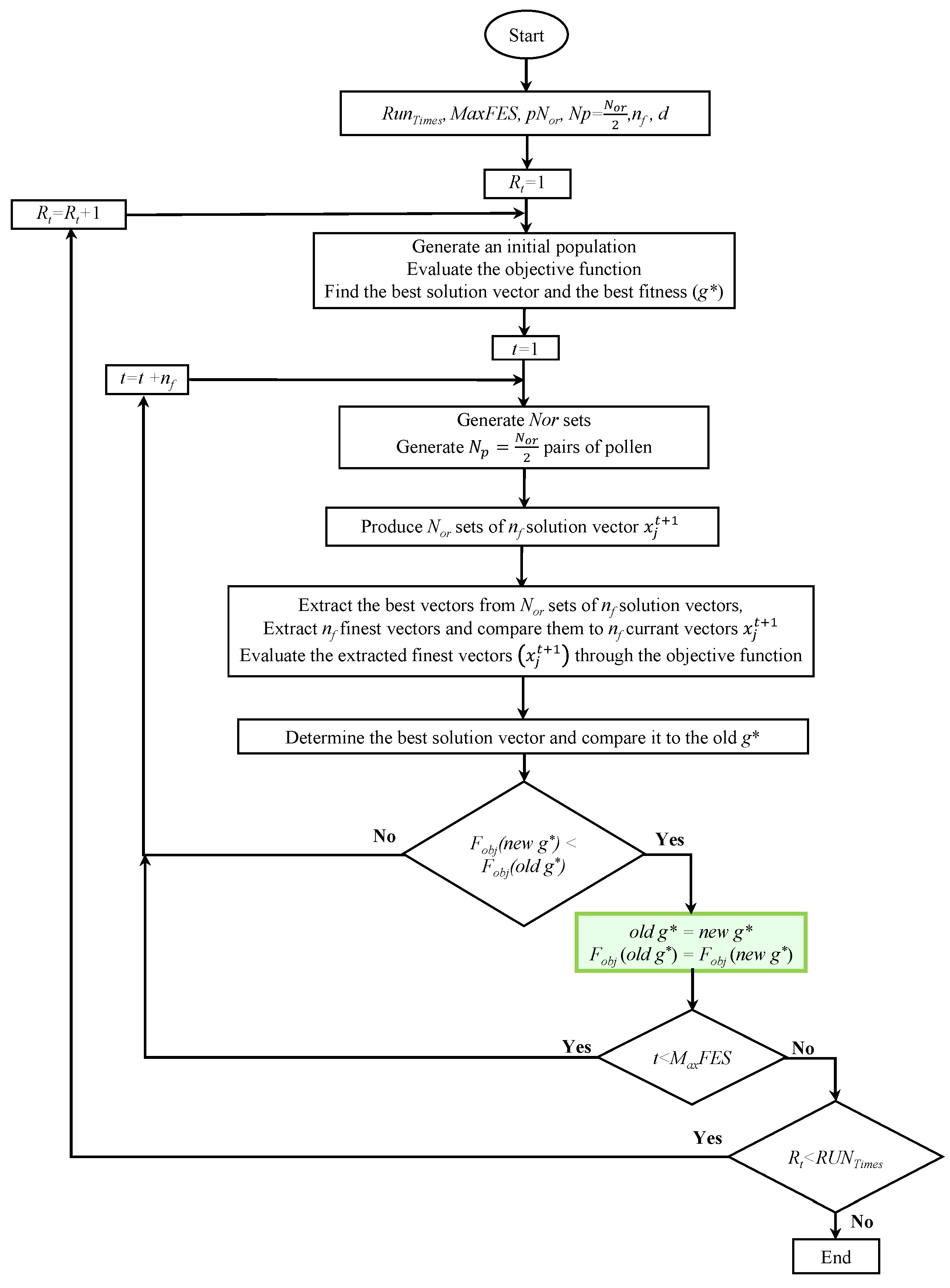
4.6. Overview of MOD-FPA

In [31], the pollination process is replaced by the generation during each iteration of a set of complete random orientations under conditions similar to FPA [43]. The main objective of MOD-FPA is to improve the performance of FPA in terms of intensification, diversification, and speed of convergence properties.

Two variations were made in the FPA process: (a) The estimation of a set of global orientations for all members of the population towards global or local pollination; (b) The construction of a set of better solution vectors related to all generated global orientations. This set is compared with each iteration with a fixed number of real solution vectors to select the best one among them based on their fitness values. In MOD-FPA two matrices are calculated at each iteration t; one contain $N_{or}$ sets, where each set is represented by a column with a random number of orientations toward global pollination. The second matrix includes the same number of sets as the first, but has $n_f-ran{d}_{Glog}$ orientations toward local pollination. Please note that the filling of each set is computed using the switch FPA parameter p.

The computed solution vector $x_i^{t+1}$, in $t+1$ requires of $(g^{\ast }-x_i^t)$ and $(x_j^t-x_k^t)$ according to (14) and (16), respectively. The MOD-FPA has been proposed to use a solution vector $x_i^{t+1}$ generated $N_p$ pairs of pollen lists extracted from different flowers of the same plants species, each iteration either using global or local pollination. This presents significant improvements to the FPA basic version in terms of found solutions quality [31]. The $N_p$$(x_j^t-x_k^t)$ terms can be generated using successively $N_p$ pairs of pollen determined at each new iteration t. However, it is important to note that each generated complete orientation is associated with a pair of pollen gametes lists. More specifically, each set number $n_o$ is assorted to the pair number $n_p$. This means that $N_{or}=2N_p$. As a result, the global exploitation algorithm characteristic is significantly enhanced. It should be noted that MOD-FPA offers the possibility to have a unique best solution generated during one cycle, either through a local or global pollination. The flow chart of MOD-FPA algorithm is shown in Figure 2. A detailed description of these processes is presented in [31].

5. Controllers Tuning Methodology

In this section, six different reactive, nature-inspired algorithms with the proposed objective function (12) are employed to search optimum values of three PI controllers for the velocity trajectory tracking controller. The block diagram of the control scheme is given in Figure 1 and PMSM parameters are given in

Table 1. PMSM nominal parameters.

Description	Symbol	Value
Inertia moment	J	$3.5$ × ${10}^{-5}$ kg/m2
Nominal voltage	v	120 V
Rated current		4 A
Stator resistance	$r_s$	$2.6$$\mathsf{\Omega }$
Stator inductance d	$L_d$	$6.73$ mH
Stator inductance q	$L_q$	$6.73$ mH
Stator dispersion inductance	$L_{ls}$	0.1$L_q$
Magnetic flux	${\lambda }_m$	$0.319$ Wb
Viscous friction coefficient	B	1.0 × ${10}^{-4}$ Nms
Direct current voltage bus	$V_{CD}$	250 V
Pole pairs	$n_p$	2

. Six parameters in velocity trajectory tracking controller can be tuned simultaneously to attain an improvement in motor performance. The control scheme, together with optimized PI are implemented using Matlab/Simulink 9.1 on Window 8.1 Professional Intel^® CoreTM i7-4712HQ CPU @ 2.3 GHz 16 GB RAM.

The parameter settings for each algorithm used in the experiment are shown in

Table 2. Parameter settings for each algorithm.

Algorithm
CSA		WOA		MOA		DA		FPA		MOD-FPA
Parameter	Set	Parameter	Set	Parameter	Set	Parameter	Set	Parameter	Set	Parameter	Set
Max num iterations	150	Max num iterations	150	Max num iterations	150	Max num iterations	150	Max num iterations	150	Max num iterations	150
$P_a$	0.25	Pop. size	50	Pop. size	50	Pop. size	50	Pop. size	50	Pop. size	50
$\alpha$	2.5	p	0.5	b	1	$\beta$	1.5	P	0.8	P	0.8
$\lambda$	1.5	b	0.95					$\beta$	1.5	$\beta$	1.5
Nests	50	$\overrightarrow{a}$ linearly decreases	2 to 0					$\lambda$	1.5	$N_{or}$	2$N_p=150$

. The six algorithms use the same objective function (12) for the optimization of each algorithm. The performance of the optimized PI controller is evaluated with objective function (12) that considers rise time, settling time, steady state error, overshoot, RMSE, JISE, JIAE, JITSE, and JITAE. The search for optimal gains is done with nominal PMSM parameters and a nominal load torque of 2 Nm. For finding the optimum values of PI parameters through MOD-FPA, DA, WOA, FPA, MOA, and CSA, 25 independent runs of each algorithm were computed so that a statistical analysis could be performed on data, see

Table 3. Results for each algorithm.

Algorithm	WOA		CSA		MOA		DA		FPA		MOD-FPA
	Fmin	Time (s)	Fmin	Time (s)	Fmin	Time (s)	Fmin	Time (s)	Fmin	Time (s)	Fmin	Time (s)
1	22.6994	9.7629	12.6686	11.1216	16.1739	100.8926	12.1782	60.3278	19.4428	61.9032	13.1286	50.8423
2	24.6300	10.0120	13.3347	20.0250	16.0381	17.8061	12.6654	173.4184	17.5573	68.5206	12.1802	53.8376
3	24.1075	9.8840	13.8902	12.9715	15.1834	19.8049	12.2521	198.9473	14.3185	68.6631	12.9781	63.3364
4	31.9663	15.9494	14.2112	25.9766	15.0710	171.1894	12.4561	65.9023	18.3437	67.9709	13.9798	56.6246
5	26.0397	10.4179	12.3965	11.5067	15.6704	42.3323	12.3193	61.3436	17.1240	68.2875	12.2019	76.9480
6	24.2628	10.2366	13.4341	13.2358	15.0166	456.2442	12.1703	62.1292	17.2445	69.3678	15.4764	66.5200
7	25.0451	15.3526	13.2952	24.3957	15.0218	401.0097	12.2335	124.8784	17.0061	68.2612	11.7130	82.0027
8	25.1760	15.9661	13.3476	33.8889	15.1331	91.3249	12.3435	159.4066	15.3419	67.6977	12.0062	73.9802
9	23.4427	12.3607	12.7400	37.0928	15.0987	57.7924	12.2090	140.4617	15.9161	68.9211	14.0449	64.1778
10	23.0715	14.2450	12.5240	23.4901	15.9019	26.4847	12.1547	155.3517	19.1114	69.5845	12.2709	57.2700
11	25.7892	16.0392	12.2125	24.7140	15.8864	53.1811	12.2761	166.6872	17.6686	69.7636	11.6044	82.5346
12	24.5148	10.2259	12.2005	13.7651	16.0996	24.5379	12.4171	62.3930	18.6116	71.2002	11.9056	60.7460
13	20.0042	13.0276	13.2360	11.0687	15.8925	22.6724	12.1286	162.2462	18.7515	69.7693	13.6080	80.2960
14	23.7718	10.0917	12.7649	21.7170	15.2064	42.8231	12.1749	144.8146	15.7143	71.5348	12.9382	88.3238
15	23.8330	11.3413	12.2352	26.7393	15.1215	53.4467	12.2862	127.0251	17.7395	70.5596	11.6248	68.3444
16	23.4915	18.3564	13.5295	16.3069	15.9487	21.4712	12.4545	184.5878	16.8993	69.4661	15.4240	85.9715
17	19.9996	28.7599	14.8069	8.9223	16.1761	23.9274	12.1259	172.1421	16.2686	69.7409	11.9933	85.0920
18	24.4517	15.3679	14.1889	12.4056	15.1758	32.2807	12.1928	183.7906	16.6907	70.4172	13.1080	67.1999
19	23.2751	9.4537	13.2900	16.4322	15.5920	26.1728	12.1271	171.7891	17.3482	69.4995	12.7458	74.1920
20	29.2304	17.1070	12.6198	11.8579	15.0467	288.8992	12.3381	154.1914	15.9538	70.7724	14.6669	57.7763
21	22.8498	9.9913	13.0761	26.2660	15.1684	84.8600	12.2090	144.6471	17.4028	68.8338	13.4155	77.1744
22	22.7927	16.1717	12.2834	17.5838	16.2844	23.1870	12.2886	168.5149	17.6001	94.7242	11.7557	61.6966
23	25.7762	15.7192	14.6626	18.8585	15.4847	36.4363	12.5411	195.4198	15.9356	94.4562	12.6093	53.6038
24	22.1067	16.0310	12.5529	31.5798	15.0241	362.9245	12.2561	175.5576	16.2506	93.0406	11.7642	50.0331
25	24.4228	17.7745	13.3719	25.2745	15.0251	280.7601	12.4785	173.8678	15.9975	97.4004	12.7630	83.3687
Minimum	19.9996	9.4537	12.2005	8.9223	15.0166	17.8061	12.1259	60.3278	14.3185	61.9032	11.6044	50.0331
Maximum	31.9663	28.7599	14.8069	37.0928	16.2844	456.2442	12.6654	198.9473	19.4428	97.4004	15.4764	88.3238
Average	24.2700	13.9858	13.1549	19.8879	15.4976	110.4985	12.2911	143.5937	17.0496	73.2143	12.8763	68.8757
Standard deviation	2.4595	4.2957	0.7555	7.8228	0.4575	134.2499	0.1418	45.2255	1.2426	9.8454	1.1349	12.1583
Variance	6.0490	18.4526	0.5709	61.1955	0.2093	18,023.0341	0.0201	2045.3484	1.5442	96.9313	1.2881	147.8247

The best results of each study and comparative analysis are highlighted in bold in the corresponding table.

.

The optimal gains value for the velocity trajectory tracking controller are tuned with six different nature-inspired algorithms are tabulated in

Table 4. Optimal value for PI controller gains using CSA, WOA, MOA, DA, MOD-FPA and FPA.

Algorithm	${\mathit{k}}_{\mathit{p},{\mathit{\omega }}_{\mathit{r}}}$	${\mathit{k}}_{\mathit{i},{\mathit{\omega }}_{\mathit{r}}}$	${\mathit{k}}_{\mathit{p},{\mathit{i}}_{\mathit{q}}}$	${\mathit{k}}_{\mathit{i},{\mathit{i}}_{\mathit{q}}}$	${\mathit{k}}_{\mathit{p},{\mathit{i}}_{\mathit{d}}}$	${\mathit{k}}_{\mathit{i},{\mathit{i}}_{\mathit{d}}}$	${\mathit{F}}_{\mathit{min}}$
CSA	1.0262	8.8369	6.9248	23.4701	7.1267	2.2591	12.2005
WOA	0.1104	46.4259	62.3245	0.1756	47.8563	0.1756	19.9996
MOA	0.2727	97.3000	11.1623	25.1522	1.3187	18.6495	15.0166
DA	0.0411	17.1440	28.1149	7.1869	12.9935	5.0739	12.1259
FPA	1.5970	88.4017	23.5742	185.9878	74.7438	194.9891	14.3185
MOD-FPA	0.4004	70.8571	39.7645	207.3428	51.864	180.338	11.6044

The best results of each study and comparative analysis are highlighted in bold in the corresponding table.

. Table 3 lists the statistical comparison between six search algorithms in terms of the best, mean, worst fitness values, and computational (CPU) time. The best results of each study and comparative analysis are highlighted in bold in the corresponding table.

The results presented in Table 3 show that MOD-FPA offered the best fitness values $\left(11.6044\right)$ compared to other nature-inspired algorithms. From these analyses, CSA has the best average computation (8.92225 s); on the other hand, WOA has the worst fitness value than MOD-FPA, MOA, DA, and FPA.

5.1. Robustness Study

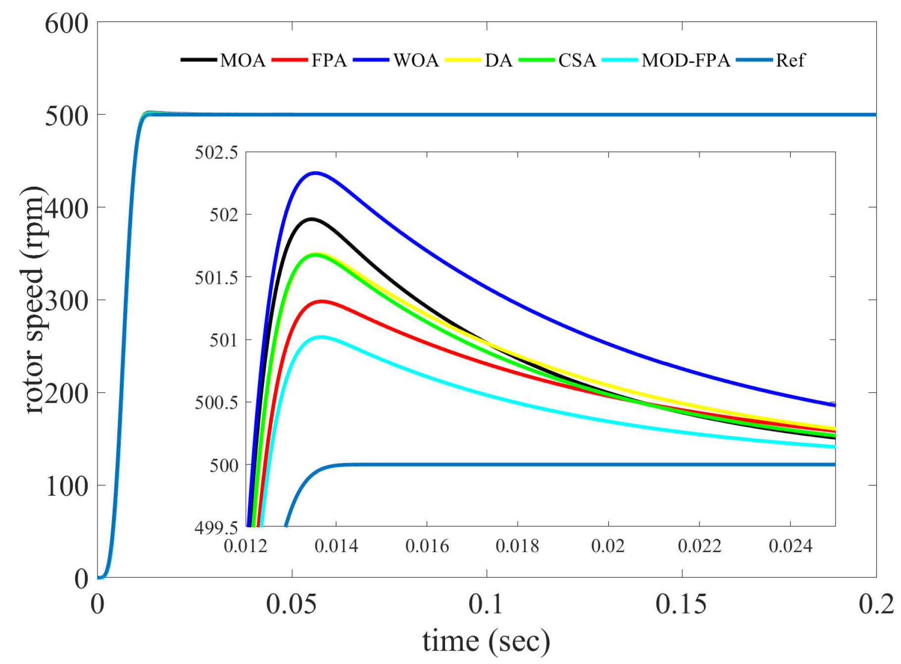
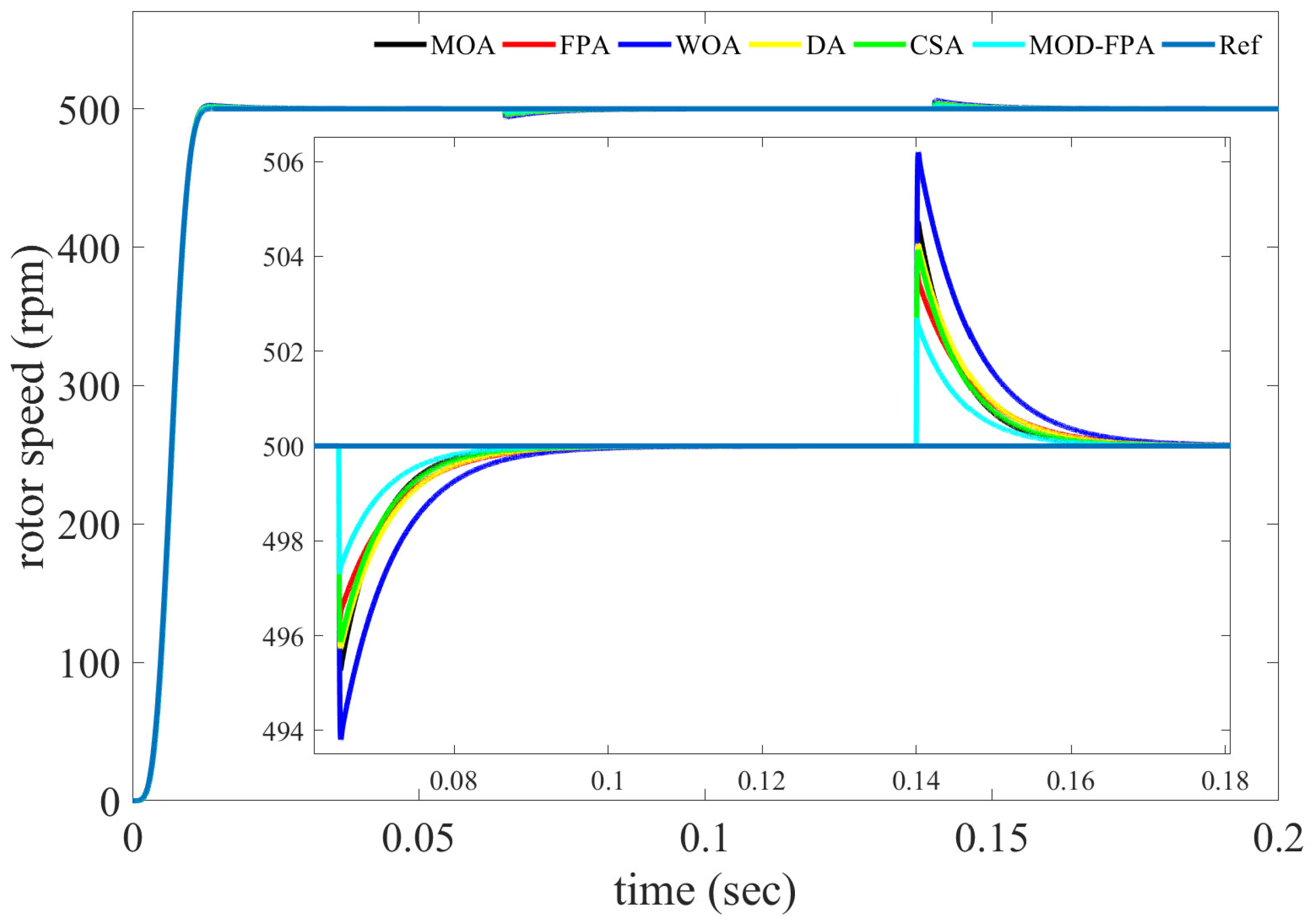
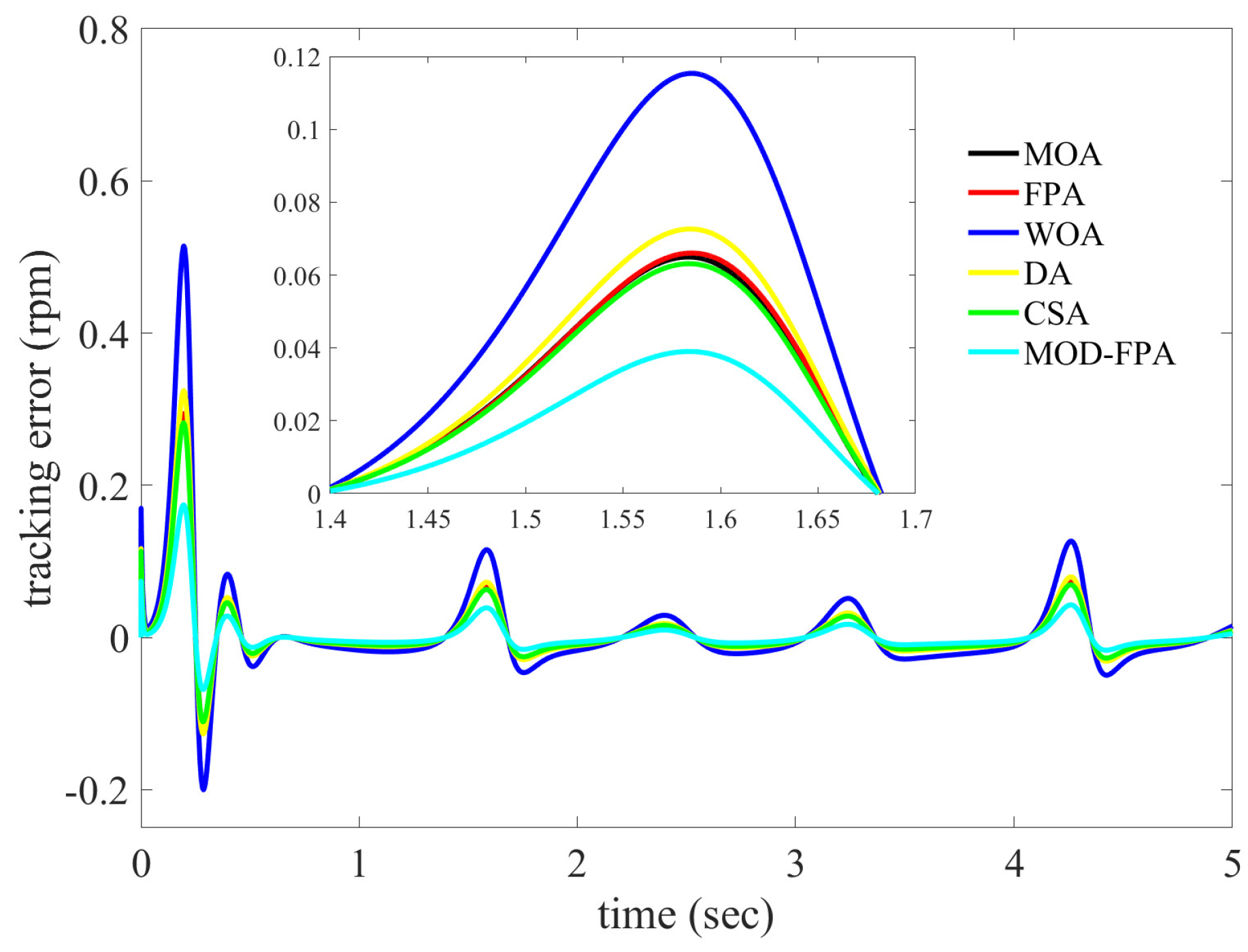
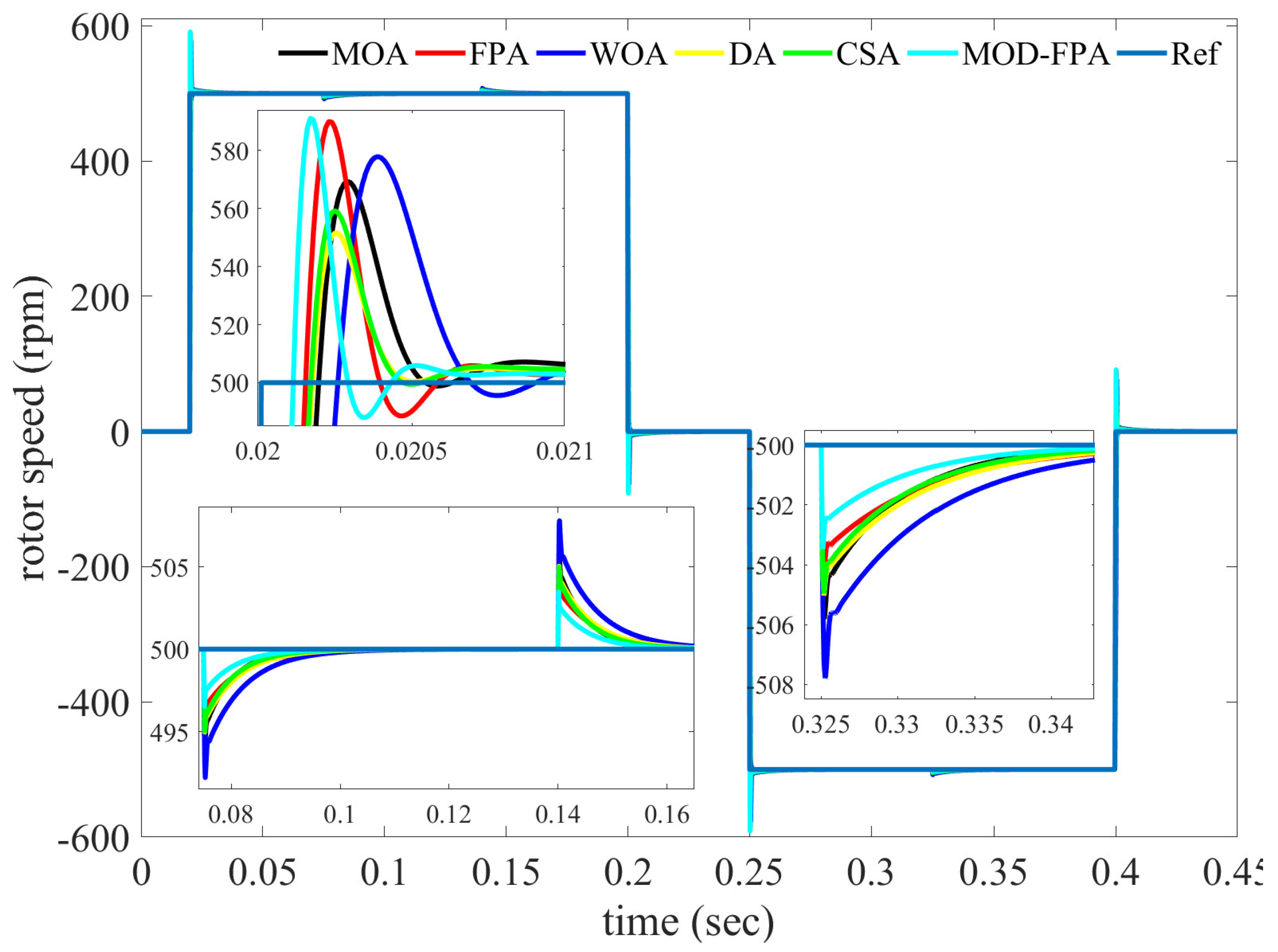
5.1.1. Simulation Result for Speed Tracking Task without Load and Nominal Parameters Condition

The velocity reference trajectory planned for the PMSM operation was specified to efficiently track the smooth motion profile defined as [45].

$${\omega }^{\ast }\left(t\right)=\left\{\begin{array}{cc}0& \mathrm{for}0\le t\le T_i\hfill \\ \tilde{\omega }\left(t,T_1,T_2\right)\overline{{\omega }_1}& \mathrm{for}{T}_i\le t\le T_f\hfill \\ \overline{{\omega }_3}& \mathrm{for}t>T_f\hfill \end{array}\right.$$

(31)

where $\overline{{\omega }_1}=500$ rpm, $T_i=0$ s, $T_f=0.02$ s, $\tilde{\omega }\left(t,T_i,T_f\right)$ is a Bézier interpolation polynomial, with $\tilde{\omega }\left(T_i,T_i,T_{i+1}\right)=0$ and $\tilde{\omega }\left(T_{i+1},T_i,T_{i+1}\right)=1$, given by

$$\begin{array}{ccc}\hfill \tilde{\omega }(t,T_i,T_{i+1})& =& {\left(\frac{t-T_i}{T_{i+1}-T_i}\right)}^5\left[d_1-d_2\left(\frac{t-T_i}{T_{i+1}-T_i}\right)\right.\hfill \\ & & \left.+d_3{\left(\frac{t-T_i}{T_{i+1}-T_i}\right)}^2-\dots -d_6{\left(\frac{t-T_i}{T_{i+1}-T_i}\right)}^5\right]\hfill \end{array}$$

with $d_1=252,$ $d_2=1050$, $d_3=1800,$ $d_4=1575,$ $d_5=700$, $d_6=126$.

Figure 3 shows the closed-loop tracking response of the velocity reference trajectory without load condition with set speed of 500 rpm of six algorithms. The performance parameter of the speed tracking task response is shown in

Table 5. Performance analysis for speed tracking task without load and nominal parameters condition.

Algorithm	MSE	JISE	JIAE	JITSE	JITAE	Rise Time	Overshoot	Settling Time	${\mathit{e}}_{\mathit{ss}}$	Overall Error Rate
MOA	0.59069	0.11814	0.04121	0.00089	0.00042	0.00561	0.39198	0.01111	0.00005	1.1601
FPA	0.38809	0.07762	0.03409	0.00058	0.00037	0.00564	0.26066	0.01117	0.00001	0.77823
WOA	1.18869	0.23775	0.05967	0.00178	0.00065	0.00561	0.46571	0.01113	0.00003	1.97103
DF	0.55037	0.11008	0.0404	0.00083	0.00043	0.00562	0.33686	0.01115	0.00004	1.05577
CSA	0.48287	0.09658	0.03757	0.00073	0.00039	0.00562	0.33492	0.01114	0.00003	0.96986
MOD-FPA	0.18572	0.03715	0.02329	0.00028	0.00024	0.00564	0.20369	0.01117	0.00001	0.4672

The best results of each study and comparative analysis are highlighted in bold in the corresponding table.

. The performance of the optimized PI controller is evaluated for trajectory tracking control in terms of time domain specifications in speed response and performance indices (MSE, JISE, JIAE, JITSE, JITAE, $t_s$, $t_r$, $M_p$ and $e_{ss}$). The main parameters, such as the overall error rate (0.46720) and overshoot (0.20369) are in favor of the MOD-FPA controller. The MOD-FPA controller has a better MSE, JISE, JIAE, JITSE, JITAE, and steady state error than other considered controllers, as shown in Table 5.

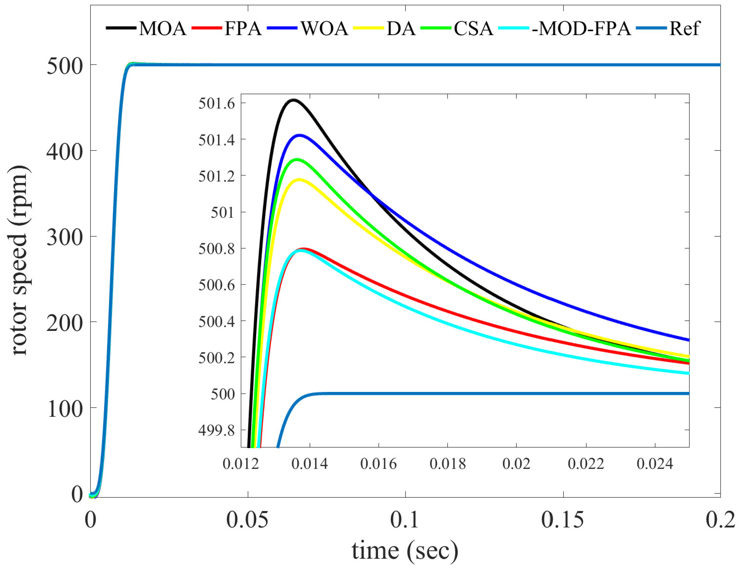
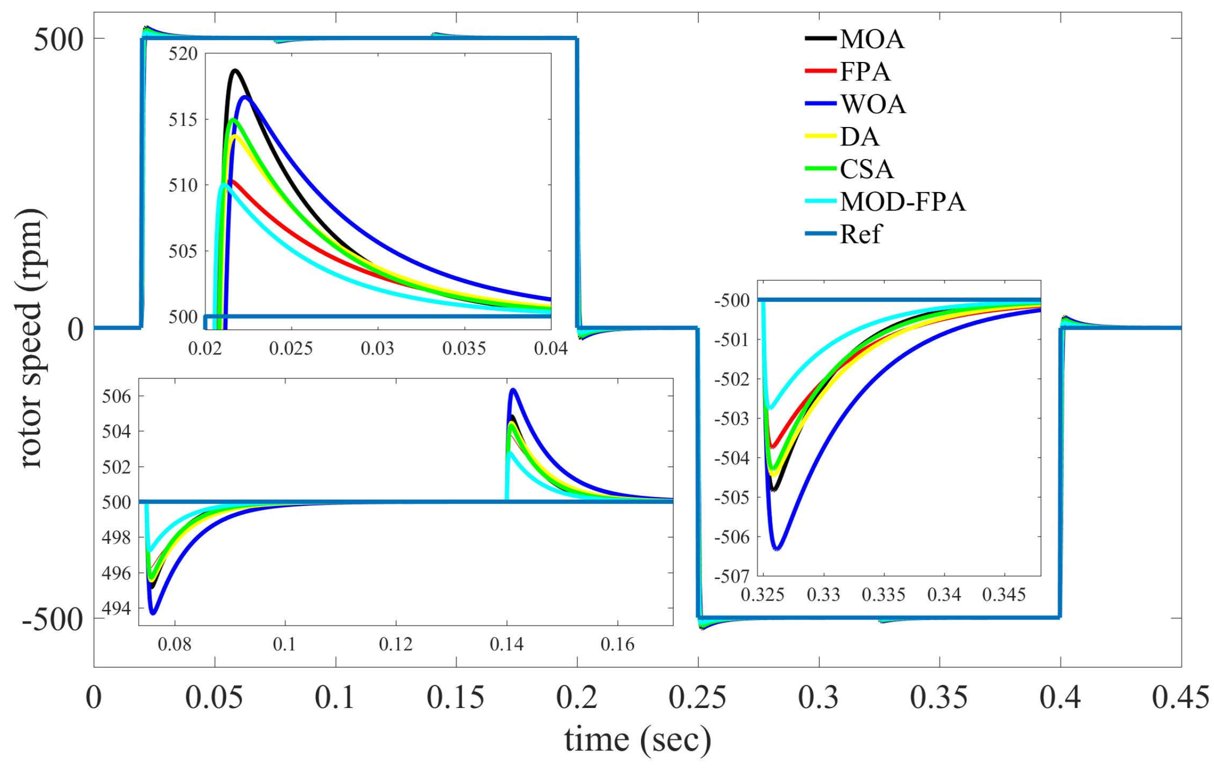
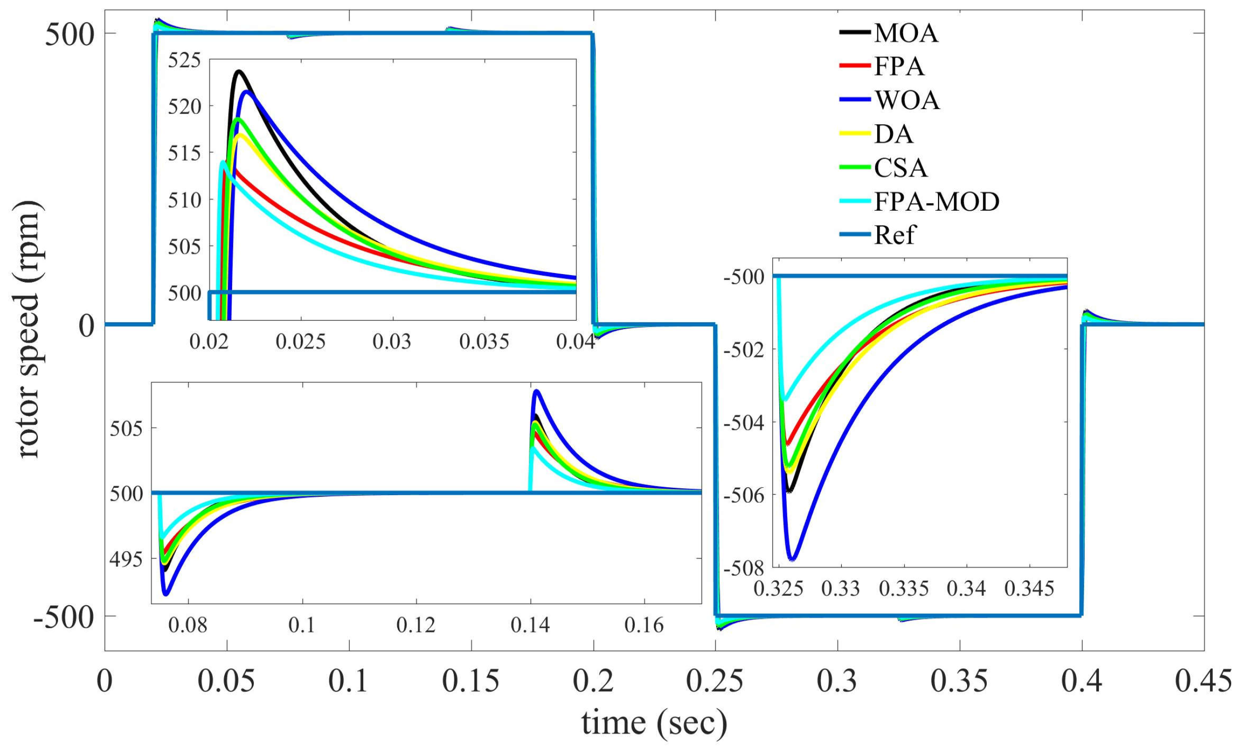
5.1.2. Simulation Result for Speed Tracking Task with Constant Load and Nominal Parameters Condition

The Figure 4 shows the closed-loop tracking response for full load (2 N.m) condition with set speed of 500 rpm. The performance parameter of the speed response is shown in

Table 6. Performance analysis for speed tracking task with constant load and nominal parameters condition.

Algorithm	MSE	JISE	JIAE	JITSE	JITAE	Rise Time	Overshoot	Settling Time	${\mathit{e}}_{\mathit{ss}}$	Overall Error Rate
MFA	1.23729	0.24747	0.05894	0.00134	0.00044	0.00558	0.32295	0.01114	0.0002	2.66301
FPA	0.8914	0.17829	0.04805	0.00096	0.00035	0.00561	0.15897	0.01122	0.00005	1.91997
WOA	2.72607	0.54524	0.08411	0.00297	0.00062	0.00557	0.28417	0.0112	0.00015	5.29016
DF	1.22334	0.24468	0.05736	0.00133	0.00043	0.00564	0.23535	0.01119	0.00019	2.56649
CSA	1.0413	0.20827	0.05359	0.00113	0.0004	0.00559	0.25751	0.01117	0.00015	2.2548
MOD-FPA	0.40039	0.08008	0.03323	0.00043	0.00025	0.00562	0.15739	0.01119	0.00008	1.0014

The best results of each study and comparative analysis are highlighted in bold in the corresponding table.

. From these results, it is clear that MOD-FPA controller has better time domain specifications in speed response and performance indices. Parameters such as overshoot, MSE, JISE, JITAE and steady state error are favoring only for MOD-FPA controller.

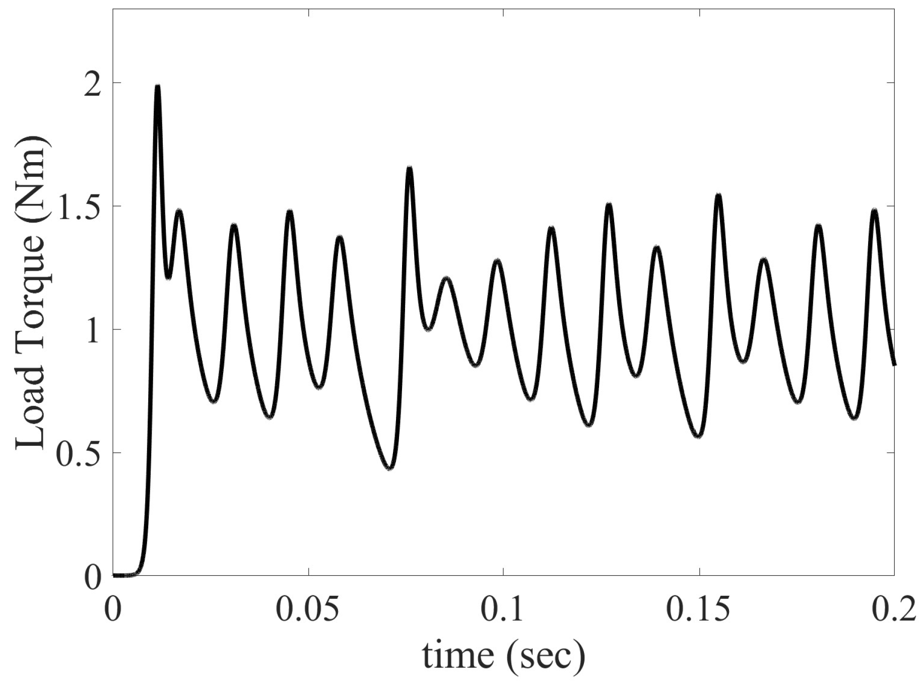
5.1.3. Simulation Result for Varying Load at Constant Speed and Nominal Parameters Condition

To validate the effectiveness of controllers, PMSM is subjected to sudden load changes also, and the response is analyzed. The speed response characteristics for varying load conditions are observed for this case. The speed is set at 500 rpm, load torque is varied from no load to full load at 0.065 s, and 0.051 s, later load torque is varied from full load to zero load. Figure 5 shows the speed response for sudden load changes condition and performance parameters are shown in

Table 7. Performance analysis for speed tracking task with constant load and nominal parameters condition.

Algorithm	MSE	JISE	JIAE	JITSE	JITAE	Rise Time	Overshoot	Settling Time	${\mathit{e}}_{\mathit{ss}}$	Overall Error Rate
MFA	1.18804	0.23762	0.09067	0.01345	0.00574	0.00561	0.94610	0.01111	0.00009	3.40021
FPA	0.83917	0.16784	0.08446	0.01015	0.00589	0.00564	0.73195	0.01117	0.00071	2.55113
WOA	2.56335	0.5127	0.1477	0.03095	0.01029	0.00561	1.23909	0.01113	0.00123	5.70655
DF	1.15618	0.23125	0.09577	0.01364	0.00645	0.00562	0.85329	0.01115	0.00035	3.1855
CSA	0.99115	0.19824	0.08565	0.01144	0.00559	0.00562	0.82687	0.01114	0.00013	2.92222
MOD-FPA	0.38175	0.07635	0.05300	0.00441	0.00345	0.00564	0.54046	0.01117	0.00008	1.58563

The best results of each study and comparative analysis are highlighted in bold in the corresponding table.

. The total performance indices are less for MOD-FPA controller than other considered controllers. Moreover, performance indices such as recovery time, overshoot, and steady state error are also in support of MOD-FPA controller.

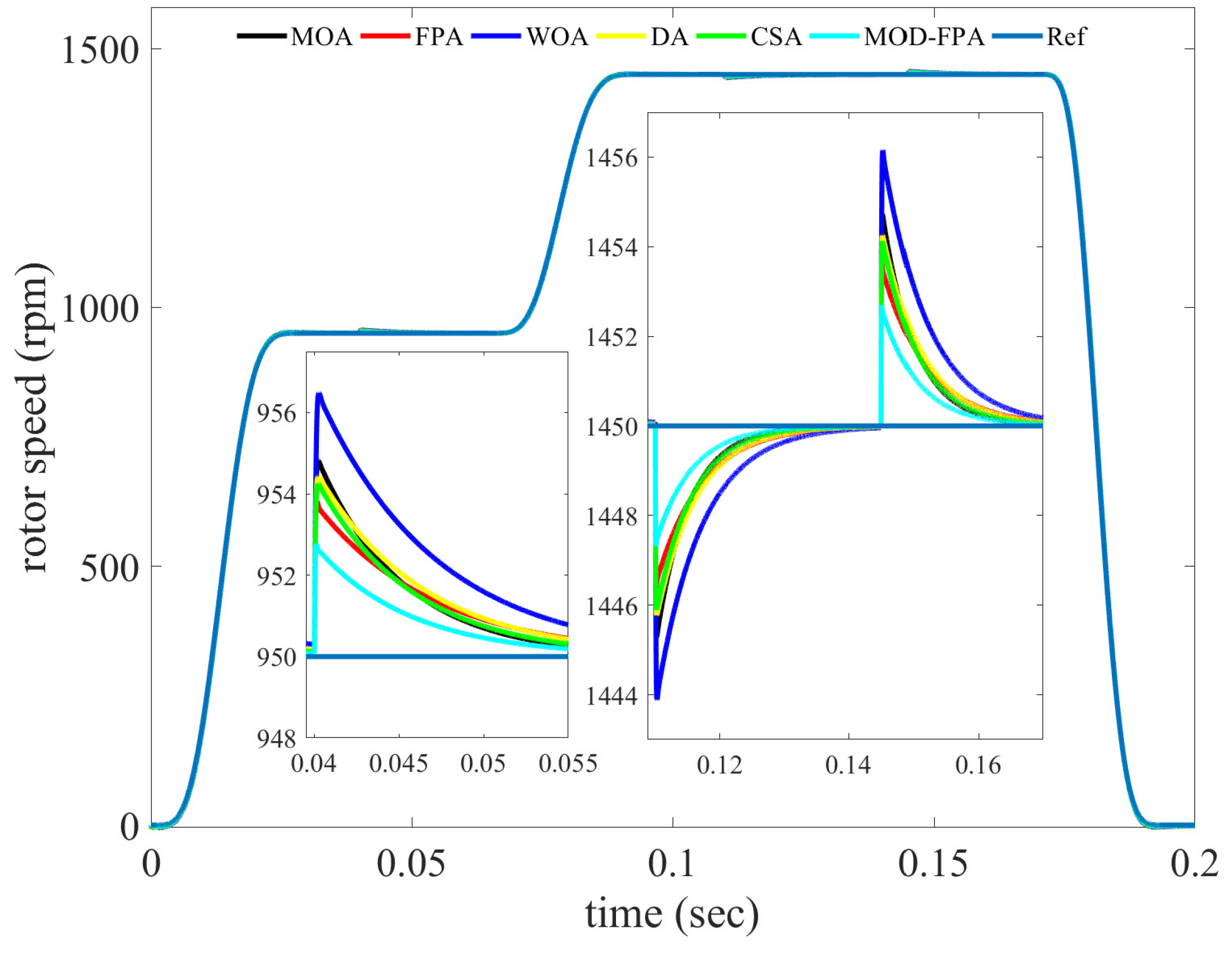
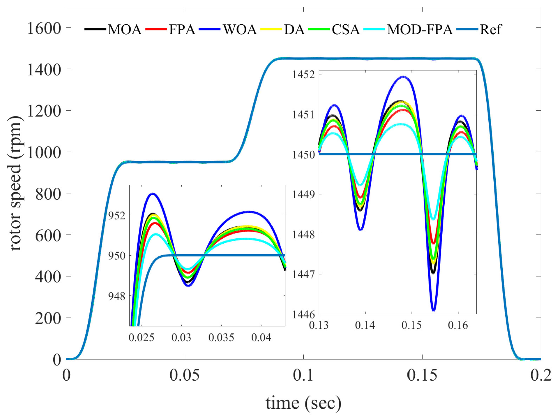
5.1.4. Simulation Result for Varying Set Rotor Speed and Load Torque, at Nominal Parameters Condition

To make the comparative analysis of the dynamic performance of the algorithms under different operating conditions, the PMSM is subjected to varying set of conditions with parameters at their nominal values. In this case, the load torque is varied suddenly three times during the simulation: (a) from 2.0 Nm to 0 Nm at 0.04 s, (b) from 0 Nm to 2.0 Nm at 0.11 s and (c) from 2.0 Nm to 0 Nm at 0.145 s The velocity reference trajectory planned for the motor operation was specified to efficiently track the smooth motion profile given by (17). The reference trajectory is taken from 950 rpm at t = 0.065 s. to 1450 rpm in a period of 0.3 s, following a Bézier polynomial trajectory. Finally, the reference trajectory is taken from 1450 rpm at t = 0.17 s to 0 rpm in 0.025 s, following a Bézier trajectory, too. The simulation results of the optimized PI controllers for speed tracking under different operating conditions are shown in Figure 6. The corresponding performance parameters are shown in

Table 8. Performance analysis for varying set rotor speed and load torque, at nominal parameters condition.

Algorithm	MSE	JISE	JIAE	JITSE	JITAE	${\mathit{e}}_{\mathit{ss}}$	Overall Error Rate
MFA	4.27836	0.85571	0.26784	0.09793	0.0272	0.66563	6.19267
FPA	3.22526	0.64509	0.24272	0.07169	0.0244	0.79300	5.00217
WOA	9.85985	1.97207	0.42451	0.21935	0.04269	1.39249	13.91096
DF	4.36026	0.8721	0.27866	0.09798	0.02811	0.85499	6.49211
CSA	3.65564	0.73117	0.25146	0.08294	0.02545	0.70312	5.44978
MOD-FPA	1.40489	0.28099	0.15569	0.03186	0.01576	0.43126	2.32046

The best results of each study and comparative analysis are highlighted in bold in the corresponding table.

. In this case, all considered parameters such as steady state error, overall error rate, MSE, JISE, JIAE, JITAE are favoring to MOD-FPA algorithm. Figure 6 exhibits that the overshoot due to external variations (load torque) is between ±3 rpm for the MOD-FPA algorithm and between ±6.4 rpm for WOA algorithm.

5.1.5. Simulation Result for Random Load Torque, Varying Set Rotor Speed and Nominal Parameters Condition

To investigate the robustness of the PI controllers, the PMSM is subjected to a random load torque, it is simulated by a the Lorenz system, described by the next first-order differential equations system [46].

$$\begin{array}{cc}\hfill & \frac{dx}{dt}=a(y-x)\hfill \\ \hfill & \frac{dy}{dt}=x(b-z)-y\hfill \\ \hfill & \frac{dy}{dt}=xy-cz\hfill \end{array}$$

(32)

where $T_l$ = 0.04z, where a = 5, b = 12 y c = 25; with initial conditions: x(0) = 0.1, y(0) = 0.1 and z(0) = 0.5. Figure 7 depicts the random perturbation load torque applied to the PMSM. The velocity reference trajectory planned for the motor operation is the same as the previous cases. The simulation results of the optimized PI controllers for speed tracking under nominal parameters and at chaotic load torque pattern are shown in Figure 8. The tracking error and the performance indices for PI controller tuned with six heuristic algorithms are shown in Figure 9 and

Table 9. Performance analysis for speed tracking task for random load torque, varying set rotor speed and nominal parameters condition.

Algorithm	MSE	JISE	JIAE	JITSE	JITAE	${\mathit{e}}_{\mathit{ss}}$	Overall Error Rate
MFA	5.51743	1.10354	0.32558	0.09823	0.03218	0.31769	7.39465
WOA	3.91025	0.78209	0.2685	0.06973	0.0265	0.11209	5.16916
FPA	11.97204	2.39453	0.46988	0.21359	0.04639	0.20831	15.30475
DF	5.40697	1.08145	0.31817	0.09649	0.03142	0.00153	6.93602
CSA	4.62539	0.92512	0.29627	0.08248	0.02927	0.14116	6.09969
MOD-FPA	1.77692	0.3554	0.18368	0.03167	0.01814	0.09578	2.46159

The best results of each study and comparative analysis are highlighted in bold in the corresponding table.

respectively. The JISE (0.00283), JIAE (0.05939), and the steady state error (0.00519) of MOD-FPA are lower than MOA, WOA, FPA, DA, and CSA algorithms as shown in Table 9. Table 9 shows clearly that the performance of the MOD-FPA is least affected by the random load torque variations as compared to MOA, WOA, FPA, DA, and CSA algorithms.

It can be inferred that the PI controllers optimized by MFA, WOA, FPA, DF, CSA, and MOD-FPA exhibit sufficient robustness despite different operating conditions.

5.2. Sensitivity Study

The sensitivity analysis is performed to determine, quantify, and analyze the transient response and performance of the PMSM when the machine is subjected under parameter uncertainty and external load disturbances. Some internal parameters (electrical and mechanical) of PMSM are changed in the range of +300% and −50% from the nominal parameters. The external load torque increases its initial value from 0 to 2 Nm, which represents its full load at t = 0.075 s; this value is maintained until t = 0.14 s, where it reaches a value of 0 Nm; finally, it increases its value from 0 to 2 Nm at t = 0.325 s; this value is maintained until t = 0.45 s. To investigate the sensitivity analysis of the implemented PI controllers, the following four cases are considered.

5.2.1. Case 1, Load Torque Is Varied from 0 to 2 Nm and Nominal Parameters

To have a point of comparison between the transient response and performance of the PMSM with nominal parameters and under parameter uncertainty, the speed response characteristics six different reactive, nature-inspired algorithms are investigated. The performance parameter of the speed response with nominal parameters and external load disturbances is shown in

Table 10. Performance analysis, Case 1.

Algorithm	MSE	JISE	JIAE	JITSE	JITAE	Rise Time	Overshoot	Settling Time	${\mathit{e}}_{\mathit{ss}}$	Overall Error Rate
MFA	12.50636	5.62799	0.38234	1.25215	0.08207	0.00013	1.72334	0.0202	0.00054	23.25371
FPA	9.93659	4.47156	0.30742	1.00099	0.06584	0.00009	3.01638	0.02026	0.00291	21.73004
WOA	16.66305	7.49854	0.52442	1.65803	0.11185	0.00017	2.19356	0.02042	0.00511	30.78568
DF	10.90907	4.90919	0.3557	1.09617	0.07615	0.00012	0.96234	0.0202	0.00192	19.25247
CSA	10.72061	4.82438	0.33895	10.77787	0.07271	0.00012	1.1434	0.02019	0.00091	28.99652
MOD-FPA	7.32725	3.29734	0.21939	0.74688	0.04731	0.00007	3.08115	0.02019	0.00053	17.71227

The best results of each study and comparative analysis are highlighted in bold in the corresponding table.

. Table 10 shows that all performance indices (MSE, JISE, JIAE, JITSE, and JITAE) and the overall error rate are lower for the MOD-FPA (17.71227). In this case, the MOD-FPA has the overshoot (3.08115) higher than the other controllers, but steady state error lower, as shown in Table 10. The time domain specification of the transient response is calculated at 0.05 s.

5.2.2. Case 2, Load Torque Is Varied from 0 to 2 Nm, $L_d=2.5L_d$, $R_s=2R_s$ and Nominal J, B, $\lambda$

The simulation results of the optimized PI controllers for closed-loop tracking response of the velocity under variations parameters ($L_d=2.5L_d$, $R_s=2R_s$) and load torque of 0 to 2.0 Nm are shown in Figure 10. The performance parameter of the speed response is shown in

Table 11. Performance analysis, Case 2.

Algorithm	MSE	JISE	JIAE	JITSE	JITAE	Rise Time	Overshoot	Settling Time	${\mathit{e}}_{\mathit{ss}}$	Overall Error Rate
MFA	17.27716	7.7749	0.4593	1.90973	0.0988	0.00013	13.86177	0.02048	0.00069	54.8034
FPA	14.42528	6.49152	0.39242	1.59971	0.0843	0.0001	17.99874	0.0205	0.00296	58.41653
WOA	23.51284	10.58101	0.64259	2.5873	0.13753	0.00017	15.58144	0.02063	0.00526	68.12983
DF	14.53939	6.54287	0.40931	1.61197	0.08779	0.00012	10.31931	0.0204	0.00208	43.50611
CSA	14.51638	6.53252	0.39766	1.60957	0.08546	0.00011	11.85184	0.0204	0.00103	46.47098
MOD-FPA	10.66016	4.79718	0.28254	1.19076	0.06102	0.00008	18.23277	0.02037	0.00059	52.87439

The best results of each study and comparative analysis are highlighted in bold in the corresponding table.

. MOD-FPA controller has lower performance indices than the other considered controllers, as shown in Table 11. Nevertheless, the percentage increase in MSE for MOD-FPA is 45.487%, and for DF algorithm the increase is 33.27%. The percentage increase in JIAE for MOD-FPA is 28.78%, and for MOA the increase is 20.12%.

5.2.3. Case 3, Load Torque Is Varied from 0 to 2 Nm, $L_d=0.8L_d$, $R_s=3R_s$, $J=3J$, $B=3B$ and $\lambda =0.9\lambda$

The simulation results of the optimized PI controllers for closed-loop tracking response of the velocity under the said parameter variations are shown in Figure 11 and

Table 12. Performance analysis, Case 3.

Algorithm	MSE	JISE	JIAE	JITSE	JITAE	Rise Time	Overshoot	Settling Time	${\mathit{e}}_{\mathit{ss}}$	Overall Error Rate
MFA	28.49916	12.82491	1.03495	4.22236	0.22567	0.00052	3.73184	0.02506	0.00153	16.95471
FPA	21.58834	9.71497	0.79872	3.20608	0.17419	0.00039	2.05505	0.02182	0.00929	11.35382
WOA	37.43438	16.84584	1.3628	5.53542	0.29695	0.00068	3.32796	0.0261	0.01558	19.17052
DF	25.47986	11.46619	0.95456	3.77837	0.20813	0.00049	2.7343	0.02389	0.00584	14.01472
CSA	24.74792	11.13681	0.91795	3.67089	0.20018	0.00046	2.98296	0.02406	0.00268	14.24489
MOD-FPA	15.85082	7.13303	0.58644	2.36369	0.12806	0.00029	1.99922	0.02047	0.00165	9.30956

The best results of each study and comparative analysis are highlighted in bold in the corresponding table.

. The percentage increase in the MSE for MOD-FPA is 159.592%, and for DF algorithm, the growth was 180.279%. The percentage increase in the JIAE for MOD-FPA is 167.304% and for MFA, the increase is 170.688%; in both cases, the time settling is less than 0.02507 s. These comparative results indicate that MOD-FPA exhibits better time response characteristics as compared to others.

5.2.4. Case 4, Load Torque Is Varied from 0 to 2 Nm, $L_d=3L_d$, $R_s=3R_s$, $J=3J$, $B=3B$ and $\lambda =0.75\lambda$

The simulation results of the optimized PI controllers for closed-loop tracking response of the velocity under variations external (Load torque is varied from 0 to 2 Nm) and internal disturbances (3$L_d$, 3$R_s$, 3J, 3B and 0.75$\lambda$) are shown in Figure 12 and

Table 13. Performance analysis, Case 4.

Algorithm	MSE	JISE	JIAE	JITSE	JITAE	Rise Time	Overshoot	Settling Time	${\mathit{e}}_{\mathit{ss}}$	Overall Error Rate
MFA	34.01983	15.30926	1.26848	4.69363	0.27648	0.00052	4.72747	0.02600	0.00174	64.88439
FPA	26.57352	11.95835	0.98649	3.67106	0.21501	0.00039	2.82158	0.02316	0.01085	48.97353
WOA	45.17517	20.32928	1.67679	6.22424	0.36527	0.00068	4.29291	0.02740	0.01782	82.23961
DF	29.75036	13.38796	1.15716	4.10735	0.2522	0.0005	3.36452	0.02507	0.00674	55.29176
CSA	29.17462	13.12887	1.11698	4.02846	0.24348	0.00047	3.70605	0.02512	0.00307	54.99965
MOD-FPA	19.56057	8.80245	0.72501	2.70932	0.15818	0.00028	2.78621	0.02228	0.00192	37.45108

The best results of each study and comparative analysis are highlighted in bold in the corresponding table.

. The percentage increase in the MSE and JITSE for MOD-FPA algorithm is 273.739%, and 262.753% is lower as compared to DF algorithm 281.797% and 274.698%, respectively. Almost all considered parameters, such as MSE, JISE, JIAE, and JITAE, favor the MOD-FPA algorithm. Compared to MFA, FPA, WOA, DF and CSA in terms of maximum overshoot, rise time and settling time, the MOD-FPA algorithm is quick and has better in disturbance rejection as observed in Figure 12 and Table 13.

As a result, the PI controller tuned by MOD-FPA using the proposed objective function outperforms PI controllers tuned with WOA, CSA, MOA, DA, and FPA optimization techniques in angular velocity tracking of the PMSM under parameter uncertainty and external load disturbances.

6. Statistical Analysis

To statistically evaluate the results obtained by the algorithms used (MOD-FPA, WOA, CSA, MOA, DA, and FPA) for the estimation of the parameters of the PI controllers. When comparing pairs, through statistical tests, we seek to establish the performance of two algorithms when applied to a common set of problems [47].

Table 14. Sing test for pairwise comparisons with a level of significance ∝ = 0.05.

MOD-FPA	WOA	CSA	MOA	DA	FPA
Wins (+)	25	17	24	10	25
Loses (−)	0	8	1	15	0

presents the critical number of wins with a ∝ = 0.05 level of significance. We established that MOD-FPA as the comparison algorithm and the table shows that this algorithm is significantly better compared to the others.

In this work, we used a non-parametric analysis called Wilcoxon test to compare two sets of ordinal data subject to different conditions [47]. For this statistical analysis, MOD-FPA algorithm is compared separately with other strategies proposed in order to test whether there is a significant difference between the proposed algorithm and the others with which it is compared. For this test, we have two hypotheses.:

• Null hypothesis ($H_0$), there is no difference between the results of the compared strategies,
• Alternative hypothesis ($H_1$), there is a difference between the results of the differentiated strategies, in other word when the null hypothesis is false.

Table 15. Wilcoxon signed rank test results with a level of significance ∝ = 0.05.

Comparison	R+	R−	p-Value	Conclusions
MOD-FPA VS WOA	0	325	$1.2290\times {10}^{-5}$	Reject the null hypothesis $H_0$
MOD-FPA VS CSA	106	219	$1.2900\times {10}^{-1}$	Retain de null hypothesis $H_0$
MOD-FPA VS MOA	2	323	$1.5705\times {10}^{-5}$	Reject the null hypothesis $H_0$
MOD-FPA VS DA	240	85	$3.7000\times {10}^{-2}$	Reject the null hypothesis $H_0$
MOD-FPA VS FPA	0	325	$1.2300\times {10}^{-5}$	Reject the null hypothesis $H_0$

shows the R+, R−, and the p-values computed for all pairwise comparisons concerning MOD-FPA. As the table states, MOD-FPA exhibits a significant improvement over WOA, CSA, MOA and FPA on the other hand; DA algorithm shows a better performance than MOD-FPA on average with a level of significance ∝ = 0.05. Another non-parametric statistical test called Friendman’s test was also performed [48]. In this test, a two-way analysis of the variations by ranges is performed. The statistical test is performed in the second step using the calculated ranges. In this test, a low range implies a better algorithm [34].

Table 16. Friedman Ranks.

P = 0.000
Treatment	Median	Sum of Ranks
WOA	24.083	150
CSA	13.226	63
DA	12.37	39
FPA	17.073	124
MOA	15.531	100
MOD-FPA	12.734	49

The best results of each study and comparative analysis are highlighted in bold in the corresponding table.

shows the Friedman Ranks.

The p-value is less than the level of significance 0.05, the null hypothesis is rejected, and it is concluded that at least 1 of the 6 algorithms has a different effect. The mean for DA and MOD-FPA are lowers and indicates that it could be more effective than other algorithms.

Finally, a post-hoc test was performed called Nemenyi test [49]. The results obtained show that there is a significant difference between the tests as shown in

Table 17. Multiple comparisons through Nemenyi Test.

Comparison	Difference in Rank Sum (DRS)	Standard Error (SE)	DRS/SE	Critical Q Value at 0.05 Level	Conclusions
WOA VS CSA	2171	217.22684	9.99416094	3.658	Reject the null hypothesis $H_0$
WOA VS MOA	1206	217.22684	5.55180014	3.658	Reject the null hypothesis $H_0$
WOA VS DA	2810	217.22684	12.9357864	3.658	Reject the null hypothesis $H_0$
WOA VS FPA	702	217.22684	3.23164486	3.658	Retain de null hypothesis $H_0$
WOA VS MOD-FPA	2486	217.22684	11.444258	3.658	Reject the null hypothesis $H_0$
CSA VS MOD-FPA	−965	217.22684	−4.4423608	3.658	Retain de null hypothesis $H_0$
CSA VS DA	639	217.22684	2.94162545	3.658	Retain de null hypothesis $H_0$
CSA VS FPA	−1469	217.22684	−6.7625161	3.658	Retain de null hypothesis $H_0$
CSA VS MOD-FPA	315	217.22684	1.45009705	3.658	Retain de null hypothesis $H_0$
MOA VS DA	1604	217.22684	7.38398625	3.658	Reject the null hypothesis $H_0$
MOA VS FPA	−504	217.22684	−2.3201553	3.658	Retain de null hypothesis $H_0$
MOA VS MOD-FPA	1280	217.22684	5.89245786	3.658	Reject the null hypothesis $H_0$
DA VS FPA	−2108	217.22684	−9.7041415	3.658	Retain de null hypothesis $H_0$
DA VS MOD-FPA	−324	217.22684	−1.4915284	3.658	Retain de null hypothesis $H_0$
FPA VS MOD-FPA	1784	217.22684	8.21261314	3.658	Reject the null hypothesis $H_0$

, except for DA and MOD-FPA, whose performance is similar. If we consider the sum of ranges, we conclude that the DA test is slightly better than the other algorithms.

After performing the nonparametric statistical analysis, we find than the DA and MOD-FPA algorithms have a statistically best performance result than other algorithms.

7. Conclusions

In this paper, the implementation of six nature-inspired heuristic techniques was used to tune the six gains of three PI controllers that regulate the speed of a PMSM. To find the optimal six gains, six particle swarm intelligence algorithms were taken into account: MOD-FPA, CSA, WOA, MOA, DA, and FPA. To verify the performance, 25 independent runs of each algorithm were done so that a statistical analysis could be performed on data. The performance of the optimized PI controller was evaluated for trajectory tracking control in terms of integral squared error (JISE), integral absolute error (JIAE), integral time absolute error (JITAE), and integral time squared error (JITSE). The effectiveness and performance of these algorithms were tested under nominal parameters with constant load torque and external load disturbances. The results of these algorithms were statistically analyzed in order to get the best algorithm. The analysis of the statistical results shows that MOD-FPA is better than CSA, WOA, MOA, FPA, DA in terms of the fitness value, JISE, JIAE, JITAE, and JITSE metrics. It should be mentioned that the six algorithms present with excellent performance, so there would be no preference or problem of using each of them indistinctly in the process of tuning the PI controllers.

References

1. Wang, G.; Zhan, H.; Zhang, G.; Gui, X.; Xu, D. Adaptive Compensation Method of Position Estimation Harmonic Error for EMF-Based Observer in Sensorless IPMSM Drives. IEEE Trans. Power Electron. 2014, 29, 3055–3064. [Google Scholar] [CrossRef]
2. Wu, Y.J.; Li, G.F. Adaptive disturbance compensation finite control set optimal control for PMSM systems based on sliding mode extended state observer. Mech. Syst. Signal Process. 2018, 98, 402–414. [Google Scholar] [CrossRef]
3. Bolognani, S.; Calligaro, S.; Petrella, R. Adaptive flux-weakening controller for IPMSM drives. In Proceedings of the 2011 IEEE Energy Conversion Congress and Exposition, Phoenix, AZ, USA, 17–22 September 2011; pp. 2437–2444. [Google Scholar]
4. Kim, J.; Jeong, I.; Lee, K.; Nam, K. Fluctuating Current Control Method for a PMSM Along Constant Torque Contours. IEEE Trans. Power Electron. 2014, 29, 6064–6073. [Google Scholar] [CrossRef]
5. Mendoza-Mondragón, F.; Hernández-Guzmán, V.M.; Rodríguez-Reséndiz, J. Robust Speed Control of Permanent Magnet Synchronous Motors Using Two-Degrees-of-Freedom Control. IEEE Trans. Ind. Electron. 2018, 65, 6099–6108. [Google Scholar] [CrossRef]
6. Ye, S. A novel fuzzy flux sliding-mode observer for the sensorless speed and position tracking of PMSMs. Optik 2018, 171, 319–325. [Google Scholar] [CrossRef]
7. Quang, N.P.; Dittrich, J.A. Vector Control of Three-Phase AC Machines System Development in the Practice, 2nd ed.; Springer International Publishing: Berlin/Heidelberg, Germany, 2015; Chapter 5; pp. 1–364. [Google Scholar]
8. Krishnan, R. Permanent Magnet Synchronous and Brushless DC Motor Drives, 2nd ed.; CRC Press: Boca Raton, FL, USA, 2010; Chapter 3; pp. 1–611. [Google Scholar]
9. Ortega, R.; Monshizadeh, N.; Monshizadeh, P.; Bazylev, D.; Pyrkin, A. Permanent magnet synchronous motors are globally asymptotically stabilizable with PI current control. Automatica 2018, 98, 296–301. [Google Scholar] [CrossRef] [Green Version]
10. Mohanty, B. Performance analysis of moth flame optimization algorithm for AGC system. Int. J. Model. Simul. 2019, 39, 73–87. [Google Scholar] [CrossRef]
11. Sabir, M.M.; Ali, T. Optimal PID controller design through swarm intelligence algorithms for sun tracking system. Appl. Math. Comput. 2016, 274, 690–699. [Google Scholar] [CrossRef]
12. Dash, P.; Saikia, L.C.; Sinha, N. Flower Pollination Algorithm Optimized PI-PD Cascade Controller in Automatic Generation Control of a Multi-area Power System. Int. J. Electr. Power Energy Syst. 2016, 82, 19–28. [Google Scholar] [CrossRef]
13. Guha, D.; Roy, P.K.; Banerjee, S. Optimal tuning of 3 degree-of-freedom PID controller for hybrid distributed power system using dragonfly algorithm. Comput. Electr. Eng. 2018, 72, 137–153. [Google Scholar] [CrossRef]
14. Bingul, Z.; Karahan, O. A novel performance criterion approach to optimum design of PID controller using cuckoo search algorithm for AVR system. J. Frankl. Inst. 2018, 355, 5534–5559. [Google Scholar] [CrossRef]
15. Wang, J.J. Parameter optimization and speed control of switched reluctance motor based on evolutionary computation methods. Swarm Evol. Comput. 2018, 39, 86–98. [Google Scholar] [CrossRef]
16. Hassanzadeh, M.E.; Hasanvand, S.; Nayeripour, M. Improved optimal harmonic reduction method in PWM AC–AC converter using modified Biogeography-Based Optimization Algorithm. Appl. Soft Comput. 2018, 73, 460–470. [Google Scholar] [CrossRef]
17. Chaurasia, G.S.; Singh, A.K.; Agrawal, S.; Sharma, N. A meta-heuristic firefly algorithm based smart control strategy and analysis of a grid connected hybrid photovoltaic/wind distributed generation system. Sol. Energy 2017, 150, 265–274. [Google Scholar] [CrossRef]
18. Sahu, R.K.; Panda, S.; Padhan, S. A hybrid firefly algorithm and pattern search technique for automatic generation control of multi area power systems. Int. J. Electr. Power Energy Syst. 2015, 64, 9–23. [Google Scholar] [CrossRef]
19. Yaghoobi, S.; Mojallali, H. Tuning of a PID controller using improved chaotic Krill Herd algorithm. Optik 2016, 127, 4803–4807. [Google Scholar] [CrossRef]
20. Dubey, H.M.; Pandit, M.; Panigrahi, B. Hybrid flower pollination algorithm with time-varying fuzzy selection mechanism for wind integrated multi-objective dynamic economic dispatch. Renew. Energy 2015, 83, 188–202. [Google Scholar] [CrossRef]
21. Mohanty, S.; Subudhi, B.; Ray, P.K. A New MPPT Design Using Grey Wolf Optimization Technique for Photovoltaic System Under Partial Shading Conditions. IEEE Trans. Sustain. Energy 2016, 7, 181–188. [Google Scholar] [CrossRef]
22. Hossain, M.A.; Ferdous, I. Autonomous robot path planning in dynamic environment using a new optimization technique inspired by bacterial foraging technique. Robot. Auton. Syst. 2015, 64, 137–141. [Google Scholar] [CrossRef]
23. Zhao, J.; Lin, M.; Xu, D.; Hao, L.; Zhang, W. Vector Control of a Hybrid Axial Field Flux-Switching Permanent Magnet Machine Based on Particle Swarm Optimization. IEEE Trans. Magn. 2015, 51, 1–4. [Google Scholar] [CrossRef]
24. Costa, B.L.G.; Bacon, V.D.; da Silva, S.A.O.; Angélico, B.A. Tuning of a PI-MR Controller Based on Differential Evolution Metaheuristic Applied to the Current Control Loop of a Shunt-APF. IEEE Trans. Ind. Electron. 2017, 64, 4751–4761. [Google Scholar] [CrossRef]
25. Zhang, D.L.; Tang, Y.G.; Guan, X.P. Optimum Design of Fractional Order PID Controller for an AVR System Using an Improved Artificial Bee Colony Algorithm. Acta Autom. Sin. 2014, 40, 973–979. [Google Scholar] [CrossRef]
26. Mirjalili, S.; Lewis, A. The Whale Optimization Algorithm. Adv. Eng. Softw. 2016, 95, 51–67. [Google Scholar] [CrossRef]
27. Dhyani, A.; Panda, M.K.; Jha, B. Moth-Flame Optimization-Based Fuzzy-PID Controller for Optimal Control of Active Magnetic Bearing System. Iran. J. Sci. Technol. Trans. Electr. Eng. 2018, 42, 451–463. [Google Scholar] [CrossRef]
28. Hasanien, H.M. Whale optimisation algorithm for automatic generation control of interconnected modern power systems including renewable energy sources. IET Gener. Transm. Distrib. 2018, 12, 607–614. [Google Scholar] [CrossRef]
29. Yousri, D.; Allam, D.; Eteiba, M. Chaotic whale optimizer variants for parameters estimation of the chaotic behavior in Permanent Magnet Synchronous Motor. Appl. Soft Comput. 2019, 74, 479–503. [Google Scholar] [CrossRef]
30. Ciabattoni, L.; Ferracuti, F.; Foresi, G.; Alessandro, F.; Monteriu, A.; Proietti, D.P. A robust and self-tuning speed control for permanent magnet synchronous motors via meta-heuristic optimization. Int. J. Adv. Manuf. Technol. 2018, 96, 1283–1292. [Google Scholar] [CrossRef]
31. Fouad, A.; Gao, X.Z. A novel modified flower pollination algorithm for global optimization. Neural Comput. Appl. 2019, 31, 3875–3908. [Google Scholar] [CrossRef]
32. Barr, R.S.; Golden, B.L.; Kelly, J.P.; Resende, M.G.C.; Stewart, W.R., Jr. Designing and reporting on computational experiments with heuristic methods. J. Heuristics 1995, 1, 9–32. [Google Scholar] [CrossRef] [Green Version]
33. Eiben, A.E.; Jelasity, M. A critical note on experimental research methodology in EC. In Proceedings of the 2002 Congress on Evolutionary Computation, Honolulu, HI, USA, 12–17 May 2002; Volume 1, pp. 582–587. [Google Scholar]
34. Derrac, J.; García, S.; Molina, D.; Herrera, F. A practical tutorial on the use of nonparametric statistical tests as a methodology for comparing evolutionary and swarm intelligence algorithms. Swarm Evol. Comput. 2011, 1, 3–18. [Google Scholar] [CrossRef]
35. Higgins, J. An Introduction to Modern Nonparametric Statistics; Duxbury Advanced Series; Brooks/Cole: London, UK, 2004. [Google Scholar]
36. Glumineau, A.; Morales, J.D.L. Sensorless AC electric motor control, robust advanced design techniques and applications. In Advances in Industrial Control, 4th ed.; Springer International Publishing: Berlin/Heidelberg, Germany, 2015; Chapter 1.4; pp. 1–244. [Google Scholar]
37. Wang, L.; Chai, S.; Yoo, D.; Gan, L.; Ng, K. PID and predictive control of electrical drives and power converters using MATLAB/simulink. In PID and Predictive Control of Electrical Drives and Power Converters Using MATLAB/Simulink; John Wiley and Sons: Hoboken, NJ, USA, 2015; Chapter 3.2; pp. 1–360. [Google Scholar]
38. Diab, A.A.Z.; Rezk, H. Global MPPT based on flower pollination and differential evolution algorithms to mitigate partial shading in building integrated PV system. Sol. Energy 2017, 157, 171–186. [Google Scholar] [CrossRef]
39. Kumar, V.; Gaur, P.; Mittal, A. ANN based self tuned PID like adaptive controller design for high performance PMSM position control. Expert Syst. Appl. 2014, 41, 7995–8002. [Google Scholar] [CrossRef]
40. Premkumar, K.; Manikandan, B. Speed control of Brushless DC motor using bat algorithm optimized Adaptive Neuro-Fuzzy Inference System. Appl. Soft Comput. 2015, 32, 403–419. [Google Scholar] [CrossRef]
41. Rajabioun, R. Cuckoo Optimization Algorithm. Appl. Soft Comput. 2011, 11, 5508–5518. [Google Scholar] [CrossRef]
42. Mirjalili, S. Dragonfly algorithm: A new meta-heuristic optimization technique for solving single-objective, discrete, and multi-objective problems. Neural Comput. Appl. 2016, 27, 1053–1073. [Google Scholar] [CrossRef]
43. Xin-She, Y. Flower Pollination Algorithm for Global Optimization. In International Conference on Unconventional Computing and Natural Computation; Springer: Berlin/Heidelberg, Germany, 2012; Volume 7445, pp. 240–249. [Google Scholar] [CrossRef] [Green Version]
44. Mirjalili, S. Moth-flame optimization algorithm: A novel nature-inspired heuristic paradigm. Knowl. Based Syst. 2015, 89, 228–249. [Google Scholar] [CrossRef]
45. Beltran-Carbajal, F.; Tapia-Olvera, R.; Lopez-Garcia, I.; Guillen, D. Adaptive dynamical tracking control under uncertainty of shunt DC motors. Electr. Power Syst. Res. 2018, 164, 70–78. [Google Scholar] [CrossRef]
46. Beltran-Carbajal, F.; Valderrabano-Gonzalez, A.; Rosas-Caro, J.; Favela-Contreras, A. An asymptotic differentiation approach of signals in velocity tracking control of DC motors. Electr. Power Syst. Res. 2015, 122, 218–223. [Google Scholar] [CrossRef]
47. Sheskin, D.J. Handbook of parametric and nonparametric statistical procedures. In Handbook of Parametric and Nonparametric Statistical Procedures, 5th ed.; CRC Press: Boca Raton, FL, USA, 2011; Chapter 6; pp. 1–1926. [Google Scholar]
48. Friedman, M. A Comparison of Alternative Tests of Significance for the Problem of m Rankings. Ann. Math. Stat. 1940, 11, 86–92. [Google Scholar] [CrossRef]
49. Zar, J.H. Biostatistical Analysis, 5th ed.; Prentice Hall: Upper Saddle River, NJ, USA, 2010; Chapter 5; pp. 1–960. [Google Scholar]
Figure 1. Schematic diagram of the permanent magnet synchronous motor (PMSM) control system.
Applsci 10 06592 g001
Figure 2. Flowchart of MOD-FPA.
Applsci 10 06592 g002
Figure 3. Speed tracking task without load and nominal parameters condition.
Applsci 10 06592 g003
Figure 4. Simulation result for speed tracking task with constant load and nominal parameters condition.
Applsci 10 06592 g004
Figure 5. Simulation result for varying load and nominal parameters conditionn.
Applsci 10 06592 g005
Figure 6. Speed Tracking Task for Varying Set Rotor Speed and Load Torque, at Nominal Parameters Condition.
Applsci 10 06592 g006
Figure 7. Random perturbation load torque applied to the PMSM.
Applsci 10 06592 g007
Figure 8. Simulation result for random load torque, varying set rotor speed and nominal parameters condition.
Applsci 10 06592 g008
Figure 9. Tracking error for random load torque, varying set rotor speed and nominal parameters condition.
Applsci 10 06592 g009
Figure 10. Simulation result for speed tracking task, Case 2.
Applsci 10 06592 g010
Figure 11. Simulation result for speed tracking task, Case 3.
Applsci 10 06592 g011
Figure 12. Simulation result for speed tracking task, Case 4.
Applsci 10 06592 g012