Abstract
Giant reeds represent a natural fiber widely available in some areas of the world. Its use can be particularly useful as the uncontrolled growth of giant reeds can be a problem because large areas are invaded by them and the crops are damaged. In this study, two models of numerical simulation of the acoustic behavior of giant reeds were put in comparison: the Hamet model and a model based on artificial neural networks. First, the characteristics of the reeds were examined and the procedures for the preparation of the samples to be analyzed were described. Then air flow resistance, porosity and sound absorption coefficient were measured and analyzed in detail. Finally, the results of the numerical modeling of the acoustic coefficient were compared. The neural network-based model showed high Pearson correlation coefficient value, indicating a large number of correct predictions.
1. Introduction
Experimental characterization and theoretical modeling of materials assumes a growing importance not only for the verification of their performance but also for the ever-greater diffusion of simulation systems and analytical forecasting methods for the design of complex systems that include these materials. The behavior of a material can be modeled using different physical, mechanical, and acoustic parameters that summarize its properties to improve the vibro-acoustic performance of the systems analyzed [1,2,3].
Sound absorbing materials have a dual function. They are used in acoustic insulation, that is, to attenuate the sound pressure level in noisy environments. They are also used for acoustic correction, that is, to control the reflections and the reverberation of the rooms. There has always been considerable interest in the materials and combined solutions used in sound absorption. Today, many efforts are made to design and produce new materials obtained from different industrial recycling methods, or from vegetable or natural fibers [4,5,6].
The solutions are designed based on the sound absorption coefficient. This is the fundamental characteristic that defines the sound-absorbing quality, which is defined as the relationship between the sound energy absorbed by the surface and the incident energy. Designing new materials therefore means testing the product by measuring the absorption coefficient and modeling its behavior to reproduce its performance in different operating conditions [7,8].
In the present work, the results obtained from the phenomenological and numerical modeling of the acoustic behavior of giant reeds shredded fibers are compared. To start, the characteristics of the models widely used for the modeling of sound-absorbing materials are reported. Then, acoustic properties’ measurements results are described. Lastly, phenomenological and numerical modeling of the acoustic coefficient are compared using the data obtained from the measurements made. The aim of this study was to produce an algorithm based on neural networks to predict the values of the acoustic absorption coefficient, known to be some characteristics of the material under examination. Algorithms based on artificial neural networks are widely used in various fields for the prediction of the behavior of nonlinear systems for which there is no rigorous mathematical model. In this research, these algorithms are used to simulate the acoustic behavior of a fibrous material obtained from giant shredded reeds for which there is no rigorous mathematical model, but only numerical models that must be adapted to this type of material.
2. Phenomenological and Numerical Models’ Descriptions
In the literature there are several models for predicting the acoustic behavior of materials. These models allow, based on the physical properties of the material, prediction of some intrinsic acoustic properties of the material, such as the complex propagation constant or the complex characteristic impedance. Three approaches were essentially adopted in the modeling of the acoustic behavior of materials: empirical, phenomenological, and numerical. In the following sections we will see some models already widely studied and a new methodological approach.
2.1. Phenomenological Model
In phenomenological models, the material is considered as an equivalent dissipative compressible fluid and no longer as a two-phase element consisting of a structure with air-filled pores inside which dissipation and heat exchange mechanisms occur. Unlike the empirical approach, the phenomenological model does not derive from a simple optimization of the experimental data but from a theoretical treatment that allows describing the phenomena of viscous friction and heat exchange. In many cases, the phenomenological approach appears to be a balanced compromise between the number of parameters necessary for modeling, modeling complexity, and forecasting ability [9]. Hamet et al. [10] proposed an extended phenomenological model based on viscosity and heat dissipation. This model requires three parameters to characterize the material: resistivity, porosity, and structure factor. The Hamet model is particularly suitable for materials with moderate porosity. According to this theory, the acoustic behavior of a rigid frame porous material is completely characterized by the specification of the characteristic impedance Zm and of the complex wave number km, as indicated in the following equations:
Here,
- is the density of air (kg/m3)
- c is the sound speed (m/s)
- is the porosity
- s is the structure factor
- = cp/cv is the ratio of the specific heat at a constant pressure and volume of the air
- f is the frequency (Hz)
In the previous formulas there is the structure factor s; for its calculation it is necessary to adopt an indirect procedure that uses the first value of the maximum of the measured absorption coefficient. The use of this procedure is necessary because of the difficulties in directly measuring this parameter [11]. Once the trend of the absorption coefficient measured as a function of the frequency is known, we can obtain the structure factor s as follows:
Here,
- c is the sound speed (m/s)
- n is an integer, n = 0 corresponds to the first value of the maximum
- d is the thickness of the sample (m)
- f2n+1 is the corresponding frequency of the first value of the maximum of the measured absorption coefficient (Hz)
In the previous formulas, and are defined as follows:
Here,
- is the resistivity (Ns/m4)
- is the porosity
- is the density of air (kg/m3)
- s is the structure factor
- is the Prandtl number
Once the characteristic impedance Zm and the complex wave number km have been calculated, we can define the acoustic impedance Z for a porous material, with a thickness of d, as follows:
Now we can define the acoustic impedance for unit area as follows:
Finally, we can define the value of the absorption coefficient for a normal incidence as follows:
As we have said, this procedure requires prior knowledge of three parameters: resistivity, porosity, and structure factor. It will therefore be necessary to experimentally measure the values of these three parameters to estimate the absorption coefficient of the material.
2.2. Numerical Model
The term numerical model means the set of the mathematical model and the related numerical solution methods, implemented in a calculation code written in a programming language and made available in the form of software. Mathematical models can have somewhat different levels of complexity. In the previous paragraphs we have seen that for some physical processes it is extremely difficult to develop a mathematical model that can simulate the acoustic behavior of some materials.
Machine learning is a branch of artificial intelligence that gathers different mechanisms that allow an intelligent machine to improve its skills and performance over time. The machine, therefore, will be able to learn to perform certain tasks by improving, through experience, its skills, responses, and functions. At the basis of machine learning there are a series of different algorithms that, starting from primitive notions, will be able to make a specific decision rather than another or perform actions learned over time. In this way it is possible to overcome the need to develop a model of the physical processes underlying the problem.
In recent years, machine learning-based algorithms have been used to deal with problems of a different nature [12,13,14,15,16,17,18,19,20,21,22]. Specifically, neural networks are a very powerful set of algorithms that allow to tackle problems in the field of classification, and of regression. These algorithms have a high processing speed and can learn the solution by analyzing a certain set of examples.
Neural networks are machine learning models that try to imitate the structure and functioning of the biological brain, consisting of large clusters of neurons connected together by axons, through the use of sets of neural units, called artificial neurons, interconnected with each other to form a network. Each neural unit relates to many others, and the connection can be reinforcing or inhibitory in relation to the activation of the units to which it is connected. Each neuron contains a function used to combine the values of all its inputs and a function, called the activation function, which returns the output of the neuron [23,24].
These networks can be seen as nonlinear mathematical functions that transform a set of independent variables x = (x1, …, xn), called network inputs, into a set of dependent variables y = (y1, …, yk), called network outputs. The precise form of these functions depends on the internal structure of the network and on a set of values w = (w1, …, wn), called weights. We can therefore write the function of the network in the following form:
Here:
- xj is the jth input
- wj is the jth weight
- b is the bias
- y is the output
The set of weights and bias represents the information that the neuron learns during the training phase and that it retains later. The function f represents the activation function, which normally consists of a threshold or limitation function which ensures that only signals with values compatible with the threshold or limit imposed can propagate to the next neuron or neurons. Typically, the activation function is a nonlinear function, and usually it is a step, a sigmoid, or a logistics function [25].
The weights are determined during the training phase based on the experience gained by the network. Training can be a very intense computational action and requires a series of examples, called training sets, whose elements are input-target pairs. The training is carried out with the search for appropriate weight values that minimize a specific error function [26,27].
Neural networks are typically structured into three parts, containing distinct amounts of neurons:
- An input layer
- A set of hidden layers
- An output layer
The input data pass through the network from the input level to the output level, going through the connections between layers, as illustrated in Figure 1.
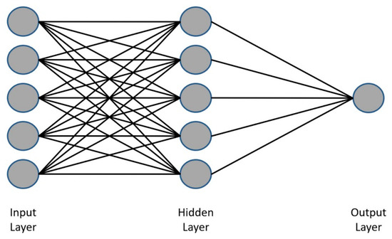
Figure 1.
Three layers Artificial Neural Network (ANN) architecture with nodes and weighted connections.
The network receives external signals on a layer of input nodes, each of which is connected to numerous internal nodes, organized in one hidden layer. Each node processes the received signals and transmits the result to subsequent nodes.
3. Materials and Methods
3.1. Giant Reeds Characterization
The giant reed (Arundo donax L.) is a perennial rhizomatous geophyte native to the Middle East, naturalized and cultivated throughout the Mediterranean basin to now be considered a typical plant of the area. This arboreal species mainly develops in environments rich in fresh or moderately brackish waters, such as along the banks of rivers and on the borders of cultivated fields. It constitutes a fundamental presence for the balance of the ecosystem of its habitat, contributing to biodiversity. The giant reed has an underground part composed of a rich system of fleshy rhizomes (5–50 cm in length) from which fibrous roots that develop over the entire surface are capable of growing in the soil up to 5 m deep, and an epigean part characterized by tall and lignified stems. The root system can grow annually from 30 to 70 cm, depending on the texture of the soil and orientation [28,29,30]. Figure 2 shows giants reeds near a river.

Figure 2.
Giants reeds near a river.
To study the acoustic characteristics, the green giant reeds were cut and shredded with a small mill. In this way, the giant reeds flake off in flakes. The shredded material has a wooden part and a part of bark. The latter comes from the outer coating of the barrel tuber which is not eliminated due to the shredding speed. At the end of the shredding operations, the material produced can come in different configurations depending on the type of mesh of the sieves installed. In this study, the shredded material was grouped into three types:
- only wooden parts with an average size of 40 mm long, 10 mm wide, and 3.0 mm thick;
- mixed composed of wooden and bark parts of various sizes;
- only parts of bark.
The shredded material is in the form of a loose granulate and is characterized by good sound absorption performance. This is because the way in which the material is arranged determines the formation of air cavities within which the sound waves can propagate and attenuate. The attenuation of the incident sound depends on the thickness, porosity, and resistance to air flow of the sample considered. Figure 3 shows the shredding operations and the average size of the crushed material.
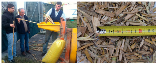
Figure 3.
Detail of the shredding operations (to the left), and the average size of the crushed material (to the right).
The flakes obtained were placed in a jute sack cone and were subsequently tested by the measuring system.
3.2. Acoustic Feature Measurements
As a first activity, measurements were made of the following acoustic properties of the material under analysis: sound absorption coefficient, resistance to air flow, and porosity. As we said, the shredded material was grouped into three types: mixed, only wooden part, and only bark. For each type, the bulk material was inserted into the sample holder with a thickness of 40 and 80 mm, respectively. Finally, six measurement sessions were performed.
For the measurement of the absorption coefficient at normal incidence, the method of the standing wave tube method (Kundt tube) was adopted. The method is described and standardized by ISO-10534-2: 1998 [31,32] and consists of generating a plane wave and measuring the sound pressure at the points where they are placed the microphones. The standard describes in detail the procedure to follow to carry out the measurement of the acoustic properties using samples of small dimensions to be assembled. The measurements were performed using a Kundt tube with a length of 56 cm and an internal diameter of 10 cm. The diameter allows measurements up to 2000 Hz while the length of the Kundt tube and the position of the two ¼ inch microphones placed at 5 cm allows measurements starting from 200 Hz. (Figure 4).
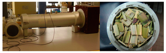
Figure 4.
Kundt’s tube for the absorbent acoustic coefficient measurement at normal incidence (to the left), and giant reeds loose material in the sample holder (to the right).
The direct wave and the reflected wave, which travel in the opposite direction inside the tube, add up vectorially by being in phase in some points and in phase opposition in others, thus generating a stationary wave. The presence of the sample inside the tube will determine the absorption of part of the incident energy. The impedance of the sample alters the way the sound is reflected and, by measuring the resulting standing wave, it will be possible to calculate the absorption coefficient at normal incidence.
Subsequently, the resistance to air flow was measured. When air passes through a material it encounters resistance; this parameter is precisely called resistance to air flow. For this measure, the procedure contained in the international standard ISO 9053: 1991 [33] was adopted. The standard offers two different methodologies for measuring this parameter. One method uses a one-way direct air flow through the material. Appropriate sensors measuring the pressure difference between the two sides of the sample return the resistance to the air flow. The other method involves an alternating air flow, with a frequency of 2 Hz. The pressure difference on the two sides of the sample positioned inside a measuring chamber is measured. The alternating air flow method was used in this study.
Figure 5 shows the instrument used to measure the resistivity of the air flow. The device consists of a closed cylindrical tube with a housing placed at the end capable of containing the sample of the material. The alternating air flow inside the tube is created by a piston system moved by a rotating cam. The difference in pressure induced is measured by a microphone placed inside the tube.
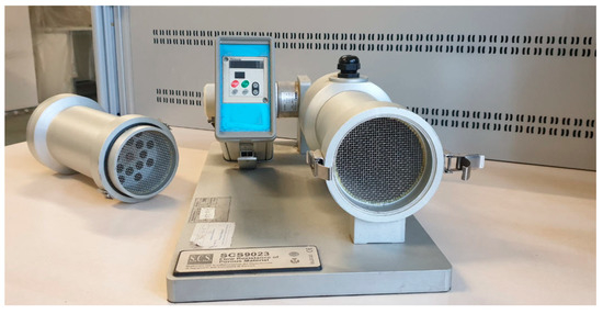
Figure 5.
Air flow resistance measurements equipment with the alternating air flow method.
Finally, porosity measurements were performed for the different sample configurations. The ratio between the volume of the fluid contained in the pores and the total volume occupied by the sample represents a definition of porosity. From this measure it is therefore possible to refer to the fraction of the volume of air inside the material. Porosity can be measured through different approaches, depending on the material used for the saturation of the pores which can be air or water, and for the procedure adopted for calculating the volume of air contained in the sample.
In this work, the porosity was calculated using the Equation (10):
Here,
- (kg/m3) is the apparent density of the material
- (kg/m3) is the density of the material
Density is defined as the ratio of mass to volume of the sample. One way to measure it is to use the apparent density obtained from the ratio between the mass of sample and the total volume of the sample. The latter is calculated by immersing the sample in a graduated glass tube containing water. From the reading of the water level, we recover the total volume of the sample. The density of the solid is calculated by a method like that used for the measurement of the apparent density. After weighing the sample, it is ground and subsequently immersed in water.
3.3. Models Comparison
After having measured the acoustic characteristics of the analyzed material, a comparison was made between the phenomenological and numerical models. For each model, the sound absorption coefficient was estimated for each configuration of the material: mixed, only wooden part, and only bark. For each type, sample holder with a thickness of 4 and 8 cm was used.
4. Results and Discussion
4.1. Measurement Results
To perform the measurements of the sound absorption coefficient, the pieces of giant reed were assembled for each of the three types (mixed, only wooden part, and only bark), obtaining six samples with thicknesses of 4 and 8 cm, respectively. The sound absorption coefficient was measured by housing the pieces of giant reed inside the Kundt tube, after which the sample was fixed to the device using an acoustically transparent grid with large meshes. Sound absorption measurement results are shown in Figure 6. Different assembled giant reed samples were measured as indicated in the Materials and Methods section.
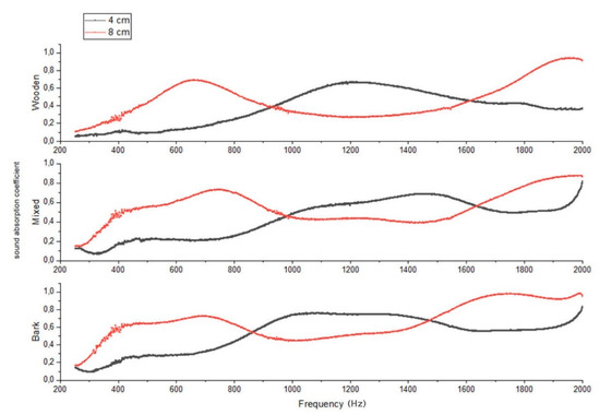
Figure 6.
Sound absorption coefficient values of 4 cm and 8 cm thick samples and for mixed, only wooden part, and only bark.
Analyzing the results of the measurement of the sound absorption coefficient shown in Figure 6, it is possible to note that the 4 cm thick samples have, under the frequency of 800 Hz, a low sound absorption coefficient value; this result is confirmed in all three types of material. On the contrary, the 8 cm thick samples show significantly higher values of the sound absorption coefficient in the same frequency range (200–800 Hz); also, in this case, this result is confirmed in all three types of material. In the frequency range 800–1500 Hz this trend reverses, in fact it is possible to notice that the sound absorption coefficient is lowered for the samples 8 cm thick and rises for the samples 4 cm thick which have higher values. Finally, at high frequencies of 1500–2000 Hz, there is a further turnaround. This time it is the values of the sound absorption coefficient of the 8 cm thick samples that have higher values.
Now let us analyze the results obtained individually for the three types of materials. Samples consisting of fragments with only one part in wood generally have values lower than 0.7 of the sound absorption coefficients. Only the sample with a thickness of 8 cm shows values higher than 0.7, and this happens starting from the frequency of 1800 Hz onwards, with a maximum value around the frequency of 1900 Hz. The samples with a thickness of 4 cm have an increasing trend at low frequencies with a maximum at the frequency of about 1200 Hz and then showing a decreasing trend at high frequencies. Samples with a thickness of 8 cm have two maximum values. High values of the sound absorption coefficient at low frequencies have a maximum near the frequency of about 650 Hz and then present a decreasing trend at medium frequencies. Starting from about 1300 Hz, this trend reverses and the sound absorption coefficient returns to increasing, with a maximum at 1950 Hz.
The samples made up of a mixture of fragments with part wood and part bark show a similar trend to the previous one. In this case, the samples with a thickness of 8 cm have two maximum values. High values of the sound absorption coefficient at low frequencies have a maximum near the frequency of about 750 Hz and then present a decreasing trend at medium frequencies. Starting from about 1500 Hz, this trend reverses and the sound absorption coefficient returns to grow with a maximum at 2000 Hz. The samples with a thickness of 4 cm show an increasing trend, with a maximum at the frequency of 1500 Hz, approximately, to then show a decreasing trend at high frequencies. Near the extreme frequency, the sound absorption coefficient starts to grow again.
Finally, the samples composed only of bark have values comparable with the previous one, even if the sample with a thickness of 8 cm shows values higher than 0.7 starting from the frequency slightly higher than 1500 Hz onwards, with a maximum value around at the frequency of 1700 Hz.
After performing the measurements on the sound absorption coefficient, we performed the resistivity and porosity measurements as indicated in the acoustic feature’s measurements section. Table 1 shows the results of the measurements.

Table 1.
Resistivity and porosity values for each type of loosed granular material (mixed, only wooden part, and only bark).
Repeated measurements were performed on four different samples. The samples were assembled by placing the bulk material in the support with a thickness of 4 and 8 cm, respectively. An average was performed from the values obtained from the measurements. Table 1 shows low flow resistance values: this is because the materials were not compressed in the sample assembly.
4.2. Phenomenological Model Simulation
After analyzing the measurement results, we proceeded to numerical simulation using the models described in detail above. As a first model, we adopted the model based on Hamet’s [10] studies. As already anticipated, this model requires knowledge of three parameters: resistivity, porosity, and structure factor. The sound absorption coefficients were calculated for each of the available frequencies in the measured values. Figure 7 shows the measured sound absorption coefficient values and those simulated with the Hamet model.
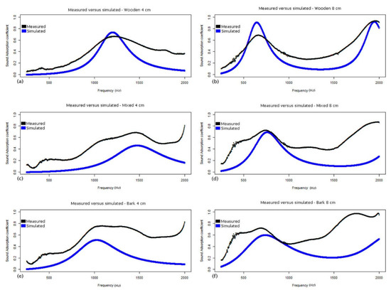
Figure 7.
Sound absorption coefficient values comparison between measured and simulated. The figure shows a 4 cm thick sample (a,c,e) and 8 cm thick sample (b,d,f) for only the wooden part (a,b), mixed (c,d), and only bark (e,f).
Analyzing Figure 7, it is possible to notice that the Hamet model can simulate the acoustic behavior of the material with different performances. The structure factor containing the information on the first maximum of the trend obtained from the measured data makes the Hamet curve consistent with the measured data. The greatest analogy between measured and simulated data occurs for the type of fragments containing only the wooden part. The 4 cm thick sample has a bell-shaped pattern, with the simulated data approaching those measured at low frequencies. The 8 cm thick sample shows a trend with a double maximum as reported by the measured data. The first maximum of the Hamet curve is positioned at the same frequency as the measured data as specified in the structure factor, but the values of the acoustic coefficient are greater. In this case, the simulated data are closer to those measured at low frequencies.
Let us now analyze the data obtained with the mixed fragments; also, in this case, the Hamet curve has a shape like that assumed by the measured data. The structure factor once again allows us to adequately position the maximum of the Hamet curve. The 4 cm thick sample has a bell shape with the simulated data which are maintained at approximately the same distance from those measured throughout the frequency interval. This behavior can be justified by a difference in the resistivity value; in fact, the Hamet model seems to refer to a lower resistivity value. The 8 cm thick sample has a bell-shaped pattern with a tail with an increasing pattern at high frequencies. Again, the simulated data is maintained at approximately the same distance from the measured data throughout the frequency range. An approach is noticeable only near the maximum.
Finally, we analyzed the data obtained with the fragments containing only bark; in this case, the Hamet curve has a shape like that assumed by the measured data. The 4 cm thick sample has a bell shape with the simulated data approaching those measured only at low frequencies. The 8 cm thick sample has a bell-shaped pattern with a tail with an increasing pattern at high frequencies. In this case, the simulated data is maintained at approximately the same distance from the measured data throughout the frequency range. An approach is noticeable only immediately after the peak of the Hamet curve.
To compare the results of the numerical modeling, we calculate the performance metrics of the model. Table 2 shows the Root Mean Square Error (RMSE), Mean Absolute Error (MAE) and the Person’s correlation coefficient for the Hamet model.
Table 2.
RMSE, MAE and the Person’s correlation coefficient for the Hamet model.
4.3. Artificial Neural Network Model
Successful prediction of data using machine learning-based algorithms essentially depends on the quality of the input data. In fact, the input data may present anomalies that in the processing phase can introduce false trends that jeopardize the prediction capacity of the model. For this reason, these anomalies must be identified and corrected in the preprocessing phase. In fact, it is necessary to identify possible anomalies such as the possible presence of any missing attributes or records, or the presence of records without values. Furthermore, since the input data contains very different variables (thickness, resistivity, porosity, frequency, sound absorption coefficient), the resizing of the data is required. This is because the input variables are characterized by different units of measurement and therefore have very different ranges of values.
The standardization of variables is crucial in statistics and data analysis. It allows us to compare variables that show different distributions, or variables with different units of measurement. In standardization, a double normalization is performed: first, the average of the distribution is subtracted from each data, therefore this difference is divided by the standard deviation of the distribution. Thus, the uniqueness of the points and the relative distances from any other point are preserved. This procedure transforms the original data into deviations from the average, and since the algebraic sum of the deviations from the average is equal to zero, it is deduced that all the standardized variables have an average of zero value. On the other hand, each gap from the mean is divided by the standard deviation of the initial variable, which means that the standard deviation of any standardized variable is equal to 1. In this work, the z score standardization has been adopted. In this way, the mean of the column was subtracted from each value in it and the result was divided by the standard deviation of the column. The Equation (11) has been applied:
In the Equation (2),
- mean (x) represent the mean of the variable x
- sd (x) is the standard deviation of the variable x
As mentioned above, standardization involves a scaling which determines the following properties:
- mean = 0
- standard deviation = 1
Standardization means that above average values will become positive scores, while below average values will become negative scores. Furthermore, the score obtained is dimensionless, simply by subtracting the mean of the distribution and dividing the result by the standard deviation of the same [25].
The purpose of this study is to produce a neural networks-based algorithm to forecast the values of the sound absorption coefficient, known to be some characteristics of the material under examination. To measure algorithm performance, model validation must be performed. It consists in verifying the model’s predictive ability using previously unused input data. The validation of the model is necessary to avoid the excess adaptation of the model; this happens when the model adapts to the observed data that has excessive parameters with respect to the observations. To get around this, we can divide the data into two subsets. The first data set, called the training set, will be used in the training phase; the second data set, called the test set, will be used in the model validation phase. The precision that we will obtain using the test data set will provide us with a measure of the model’s performance. For our needs, the input data was divided into two sets as follows: 70% of the data for training (3923 observations), and the remaining 30% of the data for validation (1681 observations). The procedure for dividing the observations was carried out completely randomly.
The simulation model was developed using an algorithm based on an artificial multilevel neural network of the feed-forward type, with one hidden layer (with 10 neurons) and an output that represents the sound absorption coefficient of the material.
During training, at each step the simulation results are compared with those obtained from the measurements. This allows you to calculate the forecast error. This error is then used to adjust the weights of the connections, trying to minimize an error function.
The adjustment of the weights is carried out as follows: first the error function derivatives are calculated with respect to the weights. Derivatives are subsequently used to calculate the new net weights. For weight regulation, the Backpropagation algorithm is the most used technique. This method uses gradient descent to search for the minimum of the error function with respect to the weights [34]. The gradient descent method identifies the direction of the maximum increase/decrease of the error function.
In this work for the regulation of weights, a variant of the conjugate gradient methods, the scaled conjugated gradient (SCG) backpropagation algorithm [35], was used. SCG returns linear convergence in most problems, returning high performance with at least one order of magnitude faster than the generic Backpropagation algorithm. This result is obtained by exploiting a step-size scaling mechanism. In this way, SCG avoids a long search per line to learn the iteration—this makes it the fastest algorithm among those most widely used. Figure 8 shows the model architecture based on neural networks.
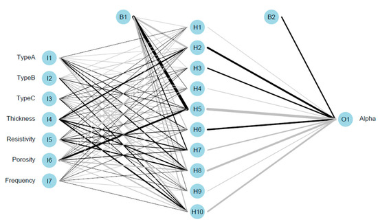
Figure 8.
Architecture of artificial neural network-based model.
Figure 8 shows the structure of each layer of the neural network. The input layer consists of seven data inputs as follows: three types of fragments (TypeA = only wooden, TypeB = mixed, TypeC = only bark), thickness of the samples, resistivity, porosity, and frequency. The hidden layer is made up of ten neurons. Finally, an output level with only one output is returned (sound adsorption coefficient). In Figure 8, the shape of the connections visually represents the strength of the weight: the greater the thickness of the line, the greater the weight. Indeed, the colors of the lines suggest the sign of the connection: black-positive; gray-negative [36,37].
Table 3 shows the RMSE, MAE and the Person’s correlation coefficient calculated for the prediction model.
Table 3.
RMSE, MAE and the Person’s correlation coefficient for the prediction model.
From the analysis of Table 3, we can see that the artificial neural network model has a decidedly low error and a high correlation between simulated data and measured data. Compared to the results obtained with the Hamet model (Table 2), we have obtained much better values.
To understand how much the simulation model manages to predict the trend of the sound absorption coefficient with the frequency, we can display the measured and simulated values to compare the results (Figure 9).
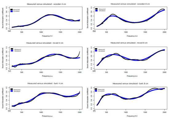
Figure 9.
Simulated versus measured sound absorption coefficients. The figure shows a 4 cm thick sample (a,c,e) and 8 cm thick sample (b,d,f) for only the wooden part (a,b), mixed (c,d), and only bark (e,f).
Let us analyze in detail the results obtained with the numerical simulation by comparing them with those obtained from the measurements with the Kundt tube. The specimens obtained by assembling only the wooden parts show excellent results for the specimen with a thickness of 4 cm. The simulated data curve fits almost perfectly on that of the measured data. Slight discrepancies occur at the high frequencies. In addition, for the 8 cm thick specimen, there is a slight underestimation of the simulated sound absorption coefficient at the peak of the bell curve.
For the specimens obtained by assembling both the wooden parts and the bark of the reeds, the simulation results return values very close to those obtained with the measurements. Once again, the 4 cm thick specimen shows better results. The deviations between the values of the simulated and measured sound absorption coefficient are greater in the case of the sample with a thickness of 8 cm. It should be noted that in this case the data obtained from the measurements show a fluctuating trend that obviously the numerical simulation model tends to optimize.
Finally, even the specimens obtained by assembling only the bark parts show satisfactory results, once again better for the 4 cm thick specimen. In the case of the sample with a thickness of 8 cm, deviations are recorded in correspondence with the peak of the bell curve at low frequency and in the vicinity of the high frequencies.
In general, the curves of the simulated data lie almost perfectly on those of the measured values. In some cases, they adapt better, for example in correspondence of anomalies due to uncertainties of the measures.
5. Conclusions
In this study, a numerical model of the acoustic properties of shredded giant reeds was developed. To begin, the models available in the literature and a new methodology based on artificial neural networks were examined. Then the characteristics of the giant reeds were analyzed and the methodology to produce the samples was characterized. Following this, a detailed description of the procedure for measuring the acoustic properties of the material was reported, and the results were analyzed in detail. In conclusion, the results of the modeling according to Hamet were compared with the results obtained from a model based on artificial neural networks.
The Pearson correlation coefficient returned by the neural network model showed high values (0.986), meaning a high number of correct predictions. The usefulness of a model for predicting the sound absorption coefficient is evident. In fact, the use of the prediction model will allow us to evaluate the acoustic performance of a material for each possible configuration, allowing a considerable saving of resources and avoiding the need to perform acoustic measurements [38,39,40].
Author Contributions
All the authors contributed to the original idea and design of the study, to the analysis, to the drafting of the manuscript, reading and approving the final version. Conceptualization, G.C., G.I., V.P.-R. and A.T.; Data curation, G.C., G.I., V.P.-R. and A.T.; Formal analysis, G.C., G.I., V.P.-R. and A.T.; Investigation, G.C., G.I., V.P.-R. and A.T.; Methodology, G.C., G.I., V.P.-R. and A.T.; Resources G.C., G.I., V.P.-R. and A.T.; Software, G.C.; Supervision, G.C., G.I., V.P.-R. and A.T.; Validation, G.C., G.I., V.P.-R. and A.T.; Visualization, G.C., G.I., V.P.-R. and A.T.; Writing—original draft, G.C., G.I., V.P.-R. and A.T.; Writing—review & editing, G.C., G.I.,V.P.-R. and A.T. All authors have read and agreed to the published version of the manuscript.
Funding
This research received no external funding.
Conflicts of Interest
The authors declare no conflict of interest.
References
- Rindel, J.H. The use of computer modeling in room acoustics. J. Vibroengineering 2000. 3, 219–224.
- Savioja, L. Modeling techniques for virtual acoustics. Simulation 1999, 45, 10. [Google Scholar]
- Egan, M.D. Architectural Acoustics; McGraw-Hill: New York, NY, USA, 1988; p. 21. [Google Scholar]
- Allard, J.; Atalla, N. Propagation of Sound in Porous Media: Modelling Sound Absorbing Materials, 2nd ed.; John Wiley & Sons: Chichester, UK, 2009. [Google Scholar]
- Sagartzazu, X.; Hervella-Nieto, L.; Pagalday, J.M. Review in sound absorbing materials. Arch. Comput. Methods Eng. 2008, 15, 311–342. [Google Scholar] [CrossRef]
- Del Rey, R.; Alba, J.; Arenas, J.P.; Sanchis, V.J. An empirical modelling of porous sound absorbing materials made of recycled foam. Appl. Acoust. 2012, 73, 604–609. [Google Scholar]
- Garai, M. Measurement of the sound-absorption coefficient in situ: The reflection method using periodic pseudo-random sequences of maximum length. Appl. Acoust. 1993, 39, 119–139. [Google Scholar] [CrossRef]
- Suhanek, M.; Jambrosic, K.; Horvat, M. A comparison of two methods for measuring the sound absorption coefficient using impedance tubes. In Proceedings of the IEEE 50th International Symposium ELMAR, Zadar, Croatia, 10–13 September 2008; Volume 1, pp. 321–324. [Google Scholar]
- Champoux, Y.; Allard, J.F. Dynamic tortuosity and bulk modulus in air-saturated porous media. J. Appl. Phys. 1991, 70, 1975–1979. [Google Scholar] [CrossRef]
- Hamet, J.F.; Berengier, M. Acoustical Characteristics of Porous Pavements: A New Phenomenological Model. In Proceedings of the 1993 International Congress on Noise Control Engineering, Leuven, Belgium, 24–26 August 1993. [Google Scholar]
- Champoux, Y.; Stinson, M.R. Measurement of tortuosity of porous materials and implications for acoustical modeling. J. Acoust. Soc. Am. 1990, 87, S139. [Google Scholar] [CrossRef]
- Iannace, G.; Ciaburro, G.; Trematerra, A. Heating, Ventilation, and Air Conditioning (HVAC) Noise Detection in Open-Plan Offices Using Recursive Partitioning. Buildings 2018, 8, 169. [Google Scholar] [CrossRef]
- Blanchet, J.; Kang, Y.; Murthy, K. Robust Wasserstein profile inference and applications to machine learning. J. Appl. Probab. 2019, 56, 830–857. [Google Scholar] [CrossRef]
- Iannace, G.; Ciaburro, G.; Trematerra, A. Fault Diagnosis for UAV Blades Using Artificial Neural Network. Robotics 2019, 8, 59. [Google Scholar] [CrossRef]
- Nichols, J.A.; Chan, H.W.H.; Baker, M.A. Machine learning: Applications of artificial intelligence to imaging and diagnosis. Biophys. Rev. 2019, 11, 111–118. [Google Scholar] [CrossRef] [PubMed]
- Puyana Romero, V.; Maffei, L.; Brambilla, G.; Ciaburro, G. Acoustic, visual and spatial indicators for the description of the soundscape of waterfront areas with and without road traffic flow. Int. J. Environ. Res. Public Health 2016, 13, 934. [Google Scholar] [CrossRef] [PubMed]
- Cardoso, P.J.; Monteiro, J.; Pinto, N.; Cruz, D.; Rodrigues, J.M. Application of Machine Learning Algorithms to the IoE: A Survey. In Harnessing the Internet of Everything (IoE) for Accelerated Innovation Opportunities; IGI Global: Hershey, PA, USA, 2019; pp. 31–56. [Google Scholar]
- Iannace, G.; Ciaburro, G.; Trematerra, A. Modelling sound absorption properties of broom fibers using artificial neural networks. Appl. Acoust. 2020, 163, 107239. [Google Scholar] [CrossRef]
- Sun, Y.; Peng, M.; Zhou, Y.; Huang, Y.; Mao, S. Application of machine learning in wireless networks: Key techniques and open issues. IEEE Commun. Surv. Tutor. 2019, 21, 3072–3108. [Google Scholar] [CrossRef]
- Iannace, G.; Ciaburro, G.; Trematerra, A. Wind Turbine Noise Prediction Using Random Forest Regression. Machines 2019, 7, 69. [Google Scholar] [CrossRef]
- Tabak, M.A.; Norouzzadeh, M.S.; Wolfson, D.W.; Sweeney, S.J.; VerCauteren, K.C.; Snow, N.P.; Halseth, J.M.; Di Salvo, P.A.; Lewis, J.S.; White, M.D.; et al. Machine learning to classify animal species in camera trap images: Applications in ecology. Methods Ecol. Evol. 2019, 10, 585–590. [Google Scholar] [CrossRef]
- Iannace, G.; Bravo-Moncayo, L.; Ciaburro, G.; Puyana-Romero, V.; Trematerra, A. The use of green materials for the acoustic correction of rooms. In Proceedings of the INTER-NOISE and NOISE-CON Congress and Conference Proceedings, Madrid, Spain, 16–19 June 2019; Volume 259, pp. 2589–2597. [Google Scholar]
- Maren, A.J.; Harston, C.T.; Pap, R.M. Handbook of Neural Computing Applications, 1st ed.; Academic Press: Cambridge, MA, USA, 2014. [Google Scholar]
- Samarasinghe, S. Neural Networks for Applied Sciences and Engineering: From Fundamentals to Complex Pattern Recognition; CRC Press: Boca Raton, FL, USA, 2016. [Google Scholar]
- Ciaburro, G.; Venkateswaran, B. Neural Networks with R: Smart Models Using CNN, RNN, Deep Learning, and Artificial Intelligence Principles; Packt Publishing Ltd.: Birmingham, UK, 2017. [Google Scholar]
- Günther, F.; Fritsch, S. Neuralnet: Training of neural networks. R J. 2010, 2, 30–38. [Google Scholar] [CrossRef]
- Han, S.; Pool, J.; Tran, J.; Dally, W. Learning both weights and connections for efficient neural network. Adv. Neural Inf. Process. Syst. 2015, 28, 1135–1143. [Google Scholar]
- Frandsen, P.R. Team Arundo: Interagency Cooperation to Control Giant Reed Cane (Arundo donax). In Assessment and Management of Plant Invasions; Springer: New York, NY, USA, 1997; pp. 244–247. [Google Scholar]
- Pilu, R.; Badone, F.C.; Michela, L. Giant reed (Arundo donax L.): A weed plant or a promising energy crop? Afr. J. Biotechnol. 2012, 11, 9163–9174. [Google Scholar]
- Pilu, R.; Cassani, E.; Landoni, M.; Badone, F.C.; Passera, A.; Cantaluppi, E.; Corno, L.; Adani, F. Genetic characterization of an Italian Giant Reed (Arundo donax L.) clones collection: Exploiting clonal selection. Euphytica 2014, 196, 169–181. [Google Scholar] [CrossRef]
- International Organization for Standardization. ISO 10534-1: Acoustics e Determination of Sound Absorption Coefficient and Impedance in Impedance Tubes-Part 1: Method Using Standing Wave Ratio; ISO: Geneva, Switzerland, 1996. [Google Scholar]
- International Organization for Standardization. ISO 10534-2: Acoustics e Determination of Sound Absorption Coefficient and Impedance in Impedance Tubes-Part 2: Transfer-function Method; ISO: Geneva, Switzerland, 1998. [Google Scholar]
- International Organization for Standardization. ISO 9053: Acoustics-Materials for Acoustical Applications-Determination of Airflow Resistance; ISO: Geneva, Switzerland, 1991. [Google Scholar]
- Riedmiller, M.; Braun, H. A direct adaptive method for faster backpropagation learning: The RPROP algorithm. In Proceedings of the IEEE international conference on neural networks, San Francisco, CA, USA, 28 March–1 April 1993; Volume 1993, pp. 586–591. [Google Scholar]
- Moller, M.F. A scaled conjugate gradient algorithm for fast supervised learning. Neural Netw. 1993, 6, 525–533. [Google Scholar] [CrossRef]
- Ripley, B.D. Pattern Recognition and Neural Networks; Cambridge University Press: Cambridge, UK, 1996. [Google Scholar]
- Venables, W.N.; Ripley, B.D. Modern Applied Statistics with S, 4th ed.; Springer: New York, NY, USA, 2002. [Google Scholar]
- Ciaburro, G.; Iannace, G.; Passaro, J.; Bifulco, A.; Marano, D.; Guida, M.; Marulo, F.; Branda, F. Artificial neural network-based models for predicting the sound absorption coefficient of electrospun poly (vinyl pyrrolidone)/silica composite. Appl. Acoust. 2020, 169, 107472. [Google Scholar] [CrossRef]
- Ciaburro, G.; Iannace, G.; Ali, M.; Alabdulkarem, A.; Nuhait, A. An Artificial neural network approach to modelling absorbent asphalts acoustic properties. J. King Saud Univ. Eng. Sci. 2020. [Google Scholar] [CrossRef]
- Iannace, G.; Ciaburro, G. Modelling sound absorption properties for recycled polyethylene terephthalate-based material using Gaussian regression. Build. Acoust. 2020. [Google Scholar] [CrossRef]
© 2020 by the authors. Licensee MDPI, Basel, Switzerland. This article is an open access article distributed under the terms and conditions of the Creative Commons Attribution (CC BY) license (http://creativecommons.org/licenses/by/4.0/).