Application of Machine Learning Techniques to Delineate Homogeneous Climate Zones in River Basins of Pakistan for Hydro-Climatic Change Impact Studies

Abstract

Climatic data archives, including grid-based remote-sensing and general circulation model (GCM) data, are used to identify future climate change trends. The performances of climate models vary in regions with spatio-temporal climatic heterogeneities because of uncertainties in model equations, anthropogenic forcing or climate variability. Hence, GCMs should be selected from climatically homogeneous zones. This study presents a framework for selecting GCMs and detecting future climate change trends after regionalizing the Indus river sub-basins in three basic steps: (1) regionalization of large river basins, based on spatial climate homogeneities, for four seasons using different machine learning algorithms and daily gridded precipitation data for 1975–2004; (2) selection of GCMs in each homogeneous climate region based on performance to simulate past climate and its temporal distribution pattern; (3) detecting future precipitation change trends using projected data (2006–2099) from the selected model for two future scenarios. The comprehensive framework, subject to some limitations and assumptions, provides divisional boundaries for the climatic zones in the study area, suitable GCMs for climate change impact projections for adaptation studies and spatially mapped precipitation change trend projections for four seasons. Thus, the importance of machine learning techniques for different types of analyses and managing long-term data is highlighted.

1. Introduction

Climate change has emerged as a major driving force behind Pakistan’s flooding over the past several decades, mainly by affecting snow melting and interfering with summer monsoon patterns [1]. Previous studies have also shown a growing interest in an accurate and calculated evaluation of climate change that can provide a rational system to adapt to a rapidly changing environment. Climate change impact analyses use long records of climate data from numerous gauging sites to estimate the historical and projected climate change trends. There is a growing institutional and social need to predict the potential impacts of climate change and the damage due to floods and droughts owing to spatio-temporal variability in the climate, specifically the rainfall. Previous studies have established that spatio-temporal dynamics in atmospheric covariates are strongly linked to the precipitation characteristics on a regional scale. The atmospheric circulation covariates are important in defining the precipitation patterns across the region [2]. Different atmospheric oscillations are responsible for this variability, which has been characterized by various climate models/simulations, including several parameters related to atmospheric oscillation moisture and wind fluxes [3]. The driver of seasonal rainfall in southeast Asia is the Monsoon circulation [4] and increases in the probability and severity of extreme events (e.g., droughts, heatwaves and floods) have been documented in several studies [5,6]. The spatio-temporal variability of the hydrological cycle parameters affects the social and environmental sustainability [7]. Therefore, the patterns and projected trends of precipitation, which is the most important variable of the hydrological cycle varies spatially as well as temporally, must be studied.

Simulation results from general circulation models (GCMs) are used to study the implications of hydro-climatic change and are considered the most comprehensive and valid instruments, with the ability to reproduce climate variables in chronological order as well as yield future projections using scenarios [8,9,10,11] recommended by the intergovernmental panel on climate change (IPCC). Numerous outputs from GCMs are available to gain insight into climate processes and the impact of various scenarios on these processes [12,13]. The question arises as to how to use these climate simulations to obtain meteorological inputs for impact models to characterize all the uncertainties involved in the models. Previous studies have reported attempts to investigate the suitability of climate models when simulating different climate parameters, such as precipitation [14]. spatio-temporal distribution by the GCM is an important aspect that must be considered for the selection of the model [15]. Further discussion regarding the selection of appropriate GCMs is presented in Section 3.2.

Climate model simulations should have adequate precision to assimilate crucial information in the observational data, which forms the basis to forecast and more efficiently predict climatic conditions. The sources of uncertainty in climate simulations and predictions are (1) model equations parameterization and initial conditions associated with chaotic systems [16]; (2) the variability in the predicted scenario caused by anthropogenic forcing, which is unknown in the future; and (3) climate variability [17]. To account for these uncertainties, multiple GCM assessment studies analyze model efficiency at simulating the dynamic and thermodynamic variables and the environmental variables related to atmospheric chemistry [4,18,19]. The common trend among the climate research community, however, is the statistical performance evaluation of GCM using climate output variables from its simulations [7,19,20,21,22,23]. These climate variables are averaged temporally and spatially on various scales for the assessment of the GCM’s ability to either simulate historical data or to present the range of climate output variables to detect a plausible future [22,24].The majority of assessment studies of climate change used the following two approaches to evaluate the climate model skill to represent past observational climate data:

• comparing the spatio-temporal average of historical/baseline observational and GCM data of different climate variables [22,25,26], using several performance indicators [27,28,29]; however, changes in the spatio-temporal average variable values may not represent the change in extreme values [30].
• comparing the observational and GCM data at each grid point [21,31,32] and then selecting the GCM in the entire study area using different filtering approaches, such as clustering hierarchy [33,34], Bayesian weighting [35], weighted skill score [15,36] and spectral analysis [37]; however, such selection processes do not cater to the area-specific efficiencies of the climate models because this efficiency varies amongst models and regions [4,27]. Several studies [21,31,32] have shown that the evaluated GCMs only account for some grid points over the entire study region. However, these studies have overlooked the ability of GCM to reproduce spatial climatic patterns. The drivers of this spatial variability are atmospheric circulation patterns that depend on the geographical location of the area. The capacity of the GCMs to reproduce the patterns of climate parameters spatially, in the baseline/historical period is, therefore, imperative [7,21]. The GCM or ensemble of GCMs selected, via the aforementioned comparative analysis of spatio-temporal averages and filtering techniques, may be appropriate for simulating the spatial climatic patterns for some percentage of the entire study area but not all, thus enhancing the uncertainties in projecting the climate. To narrow this uncertainty in projecting the climate variables (precipitation) trends, we propose a different method of the selection of GCMs by first identifying the climatologically homogeneous zones and then selecting the GCM in each zone through past performance assessment. These homogeneous sub-regions are based on similar spatial and temporal climate patterns, as depicted by the highly resolved observation data. Following the philosophy of McSweeny et al. [4] for the regional suitability of the GCMs, we selected the GCMs in every homogeneous precipitation region and validated our selection through the comparative analysis with Simple Composite Method (SCM). The SCM is broadly used for generating the multi-model ensemble that is, to obtain the equally weighted mean of all the ensemble members data at each grid point [7].

With the support of machine learning techniques, long records of climate data, from numerous gauging sites and web sources, can be easily analyzed and used to determine historical and projected trends of climate change. In the present study, the modules using machine learning techniques were developed throughout the various steps of the framework. The framework comprises five important steps: (1) developing homogeneous precipitation zones using highly resolved observation data; (2) the selection of the best suitable GCM for each zone based on the estimated correlation coefficient using the GCM data and highly resolved observed data in every homogeneous climatic region; (3) comparison and validation of the selected GCM; (4) sampling the daily precipitation data for the projected period (2006–2099); based on the forcing scenarios and (5) performing future precipitation trend detections. The outcomes of this framework are the estimated divisional boundaries of the climate zones, suitable GCMs for the climate impact studies and seasonal rainfall trend projections. It is necessary to mention that the results obtained using the present framework are subject to specific assumptions: (1) daily and 0.25° temporal and spatial scales of the data have been used for climate zoning (2) seasonal and 0.25°, temporal and spatial scales of the data have been used for the climate projection trends (3) uncertainty of the results depends on the uncertainty involved in the climate variable outputs from the GCMs. It is very important to understand the limitations and uncertainties involved in the simulation outputs of different GCMs. The present study does not aim to quantify the uncertainties present in the GCMs’ simulations but only uses the GCMs’ outputs for their selection in each climate zone and trend projections. Nonetheless, the framework can be replicated, using other versions of ensembles of GMCs’ with finer resolution and accuracy. The scientific data associated with the present framework can be shared on request.

This paper is structured as follows—Section 2 describes the study area, stations and data details; Section 3 provides a step-by-step presentation of the methodology; Section 4 presents the results and discussion; and Section 5 presents the conclusions.

2. Study Area and Data

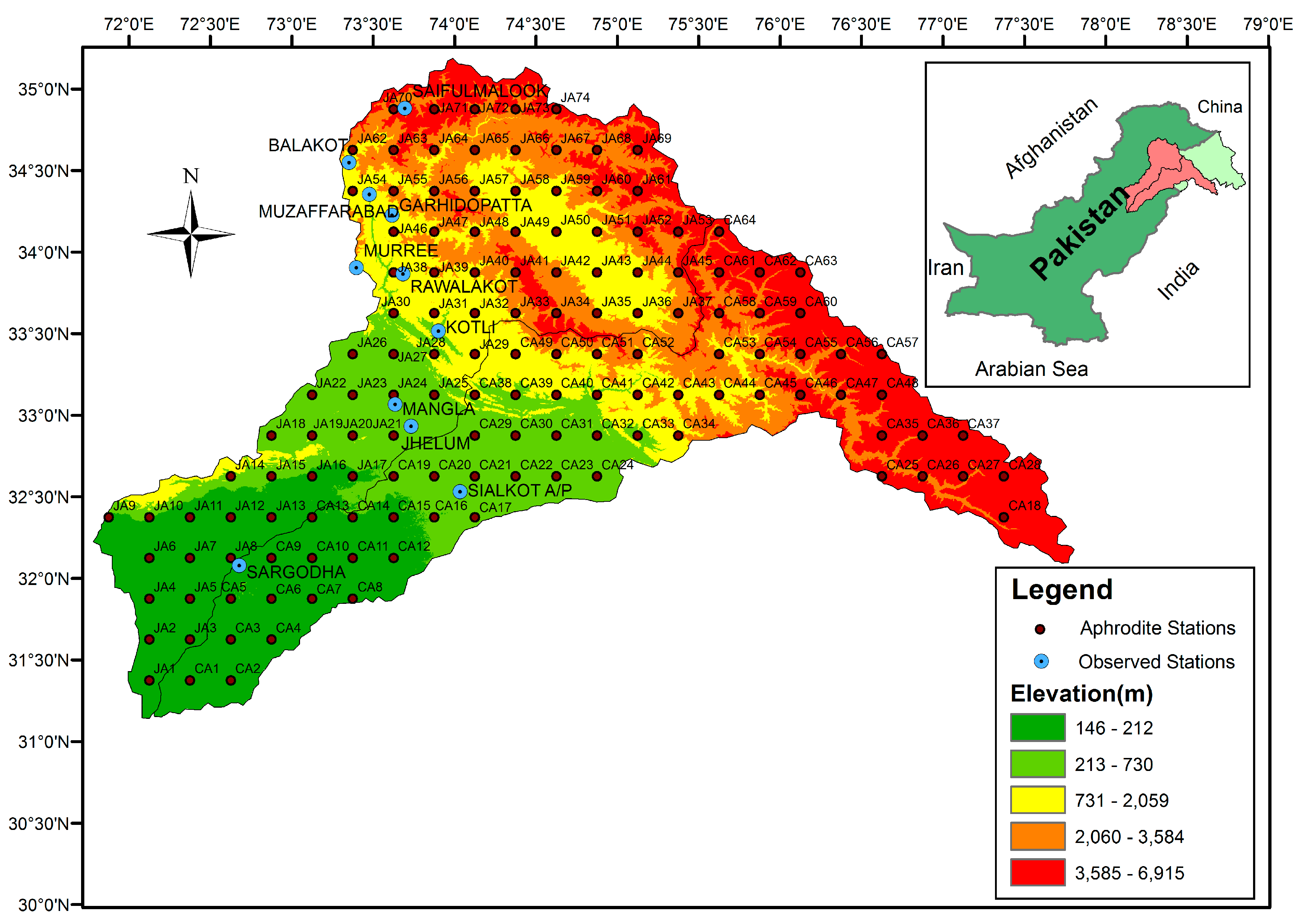
2.1. Study Area

The basin areas of the Jhelum and Chenab Rivers are 33,330 and 67,515 km², respectively. The elevations in the two basins vary between 146 and 6915 m. Figure 1 shows a topographic map with APHRODITE grid points of the basins of the Jhelum and Chenab river in Pakistan. The Southwest Monsoon triggers approximately 40% of the annual precipitation, whereas the remaining ~60% of precipitation is due to Westerly aggravations [24]. Figure 2 presents the average annual seasonal precipitation in various parts of the two basins. The spatially and temporally variable climatic conditions, atmospheric circulation, advected moisture and topography, with high elevations in the north and flat plains in the south, demand a flexible framework for the evaluation of the climate change effects and future predictions. Diminishing water resources due to high hydro-climatic variability and extreme climate events in Pakistan are some of the factors that inspired the research community to investigate sustainable solutions after analyzing future needs and availability.

2.2. APHRODITE Data

To delineate the climate zones in the study area, a dense network of data stations was required. There has been an increasing trend of using easily available gridded precipitation datasets for hydrologic and climatic assessments [38,39,40]. Previous studies have identified the performance of the APHRODITE dataset (version V1101) as the best-gridded product over the high mountainous regions of Asia [41]. To justify the use of the gridded dataset of APHRODITE, we performed the comparative analysis of the APHRODITE dataset and European Reanalysis gridded dataset (ERA5) [42] and Global Metrological forcing dataset for land surface Modeling (GMFD) [43] with the observed dataset and monthly temporal scale, at 11 gauging stations at different altitudes, as shown in Figure 1. ERA5 is also popular for its accuracy. The results of the comparative analysis have been shown in

Table 1. Comparative analysis of APHRODITE and ERA5 monthly dataset. Pearson correlation coefficients and Kolmogorov Smirnov Test results (KS Test). (The shaded p-Values are >0.05, depicting the null hypothesis of similar distribution, is not rejected).

Gauging Stations	Time Period		Correlation Coefficient			p-Value, KS Test
		Elevation (m)	APHRODITE	ERA5	GMFD	APHRODITE	ERA5	GMFD
Astore	1979–2005	2546	0.90	0.65	0.08	0.0001	0.000	0.001
Balakot	1979–2005	1088	0.91	0.77	0.17	0.018	0.069	0.000
GarhiDopatta	1979–2005	819	0.90	0.71	0.25	0.0001	0.336	0.000
Jhelum	1979–2005	234	0.99	0.79	0.31	0.99	0.000	0.238
Kotli	1979–2005	608	0.91	0.83	0.26	0.29	0.568	0.079
Mangla	1996–2005	605	0.96	0.77	0.40	0.74	0.519	0.060
Muzaffarabad	1979–2005	737	0.92	0.71	0.28	0.92	0.248	0.000
Rawalakot	2003–2005	1638	0.95	0.75	0.10	0.11	0.199	0.024
Saifulmaluk	1996–2005	3224	0.37	0.52	0.13	0.0006	0.00	0.069
Sargodha	1979–2005	190	0.78	0.75	0.26	0.0002	0.000	0.002
Sialkot	1979–2005	256	0.91	0.79	0.35	0.29	0.014	0.201

. The Pearson correlation coefficient and Kolmogorov Simirnov (KS) test (the method is discussed in Section 3.3.2) were used to compare the monthly precipitation datasets. The results tend to show agreement with the APHRODITE dataset with higher correlation coefficients at all the stations. For the KS test, p-values greater than 0.05 have been shaded, depicting the null hypothesis of similar probability distribution is not rejected. The results of comparative analysis suggests that the APHRODITE datasets have higher correlation with the observed data that is, more than 0.8 in nearly all the observed gauging station as shown in Table 1, so the APHRODITE dataset [40] of 0.25° × 0.25° spatial resolution for the period of 1970–2005 has been used at a daily temporal scale, for the delineation of climate zones. Nevertheless, the regionalization framework is equally applicable to the other datasets having comparatively higher resolution and accuracy.

Figure 2 presents the total seasonal average precipitation sampled from APHRODITE. The daily gridded precipitation long term data from 1951 and onwards, is provided by the APHRODITE product (V1101). It provides the data at the continental scale, including a dense rain gauge data network of Asia, comprising the Middle East, South and Southeast Asia with valid stations of 5000 to 12,000 [40].

2.3. NEX-GDDP-GCMs-CMIP5 Data

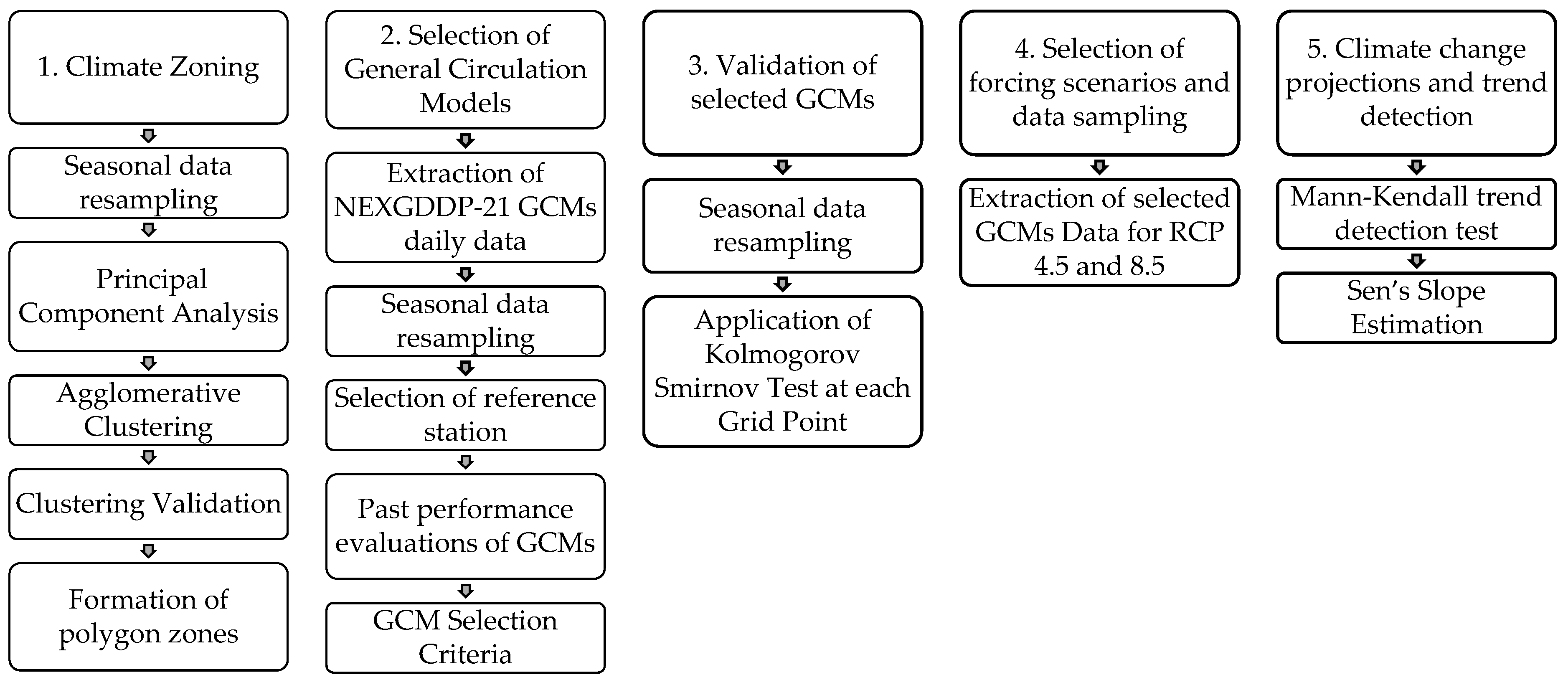
For future climate change analysis, this study used newly developed NASA Earth Exchange Global Daily Downscaled Projections (NEX-GDDP) dataset. The experiments included in Coupled Model Intercomparison Project 5 (CMIP5) were devised to address the research interrogations in AR4 of the IPCC [44]. The original resolution of most GCMs in the CMIP5 is >100 km, where such coarse resolution cannot provide fine-scale information for impact studies and decision-making at a local scale. The NEX-GDDP dataset is a collection of 21 GCMs. These datasets are bias-corrected and downscaled to a finer resolution (0.25° × 0.25°) using the bias-corrected spatial disaggregation (BCSD) method [45]. The Global Meteorological Forcing Dataset (GMFD), developed by Princeton University, provides the gridded observed climate data and the NEX-GDDP after bias correction and downscaling [46,47]. Table S1 lists the 21 GCMs in the NEX-GDDP, along with information on the research centers that produce the GCMs.

NEX-GDDP data consists of daily precipitation and minimum and maximum temperatures from historical periods (1950–2006) and future projections (2006–2099). The future projections are available for two representative concentration pathways (RCPs), which are global greenhouse gas emissions scenarios. These scenarios were employed by the IPCC fifth assessment report (AR5) [44]. The NEX-GDDP dataset is publicly available. The comprehensive details to use these scenarios dataset for climate change impact evaluations and adaptations have been provided by IPCC [48]. The CMIP5 data provides multi-model datasets of climate variability, which was used to develop AR5 [44].

3. Methodology

Machine learning algorithms are becoming more popular owing to their ability to identify the patterns and variances in large datasets composed of multivariate atmospheric covariates, location parameters, meteo-climatic information, tele-connection indices and attributes that influence precipitation [2,49,50] or the precipitation and temperature statistics [51,52]. In this study, we used the Python module scikit-learn [53], which integrates a broad range of machine learning algorithms for supervised as well as unsupervised learning. As aforementioned, this framework consists of five steps: delineation of homogeneous climate zones; selection of GCMs; validation of selected GCMs; selection of forcing Scenarios to be used for the predictions of the climate change; and climate change projections and trend detection. Figure 3 presents the methodology flow diagram adopted in this study. Further details of each step are discussed in the subsequent sections.

3.1. Climate Zoning

Climate zoning/regionalization is the most important step in this framework and the basis for the subsequent steps. For regionalization, solid evaluations of different precipitation attributes require accessibility to long records of chronicled estimations at various stations inside an area [2]. For climate zoning, 35 years’ (2006–2075) daily precipitation data of APHRODITE were used. These data were resampled seasonally to develop the climate zones for each of the seasons (defined in the subsequent sections). Regionalization was performed by grouping the rain gauges with homogeneous precipitation statistics in an area [54]. This step enables partitioning of the entire area into several climate zones for every season.

The regionalization of the precipitation statistics has numerous applications in various water resource management fields, such as agriculture practices, spatial and temporal rainfall patterns, hydrological analysis, extreme event forecasting [55] and watershed management. There are several methods available to delineate climate regions, for example, subjective and objective partitioning, geographical convenience and multivariate analysis [54,56,57]. The arbitrary and slightly misleading demarcation approach for a region, which is based on administrative boundaries and physical and geographical groupings, is referred to as the geographical convenience method. The subjective partitioning method is based on homogeneous statistical characteristics of the rainfall and previous knowledge of the region. Objective partitioning demarcates a region by grouping the sites of similar climates. Principal component analysis (PCA), clustering techniques and correlation analysis are examples of multivariate analysis techniques, which are widely used for climate zone delineation [51,58,59]. These analysis techniques require the development of a large matrix that defines the characteristics of the climate in the region. We adopted the method of PCA and agglomerative hierarchical clustering (AHC) to group the sites of homogeneous precipitation. These groups of stations were validated using different cluster validity indices.

3.1.1. Seasonal Data Resampling

The daily precipitation data in the APHRODITE time series, at 138 Grid stations in the study area from 1975–2005, were resampled as hydrological seasons: warm-wet (“July, August and September”), cold-dry (October, November and December), cold-wet (January, February and March) and warm-dry (April, May and June). The daily precipitation data of 35 years were resampled in a seasonal cycle using simple Python code.

3.1.2. Principal Component Analysis (PCA)

The benefits associated with the PCA are as follows—(1) identification of spatially coherent variations that can improve the signals, where the leading components represent the maximum variance in the patterns; (2) explanation of the covariance between the variables at various places; and (3) reduction of dimensionality, thereby providing resources to describe the variability in large spatially dimensional datasets with a reduced number of principal components [60]. PCA can present all the data in a smaller matrix and attempts to retain as much information about the data as possible. We used the dimensions from 138 APHRODITE grid point datasets for PCA. The aim was to project the data onto different orthogonal axes known as principal components. A linear transformation is performed using a symmetric covariance matrix, developed from the dataset, into the principal orthogonal components. The direction of principal components is represented by eigenvectors and the eigenvalues represent the magnitude of the stretch of the axis. This gives the direction (eigenvector) and magnitude (eigenvalue) of the spread of the dataset. The leading principal component, which presents the maximum spread of the dataset, is used for further analysis. Several principal components were selected for use in hierarchical clustering using the scree plot, which shows the variance explained in percentage by each of the principal components. Each principal component has component scores for every station, based on the eigenvectors and eigenvalues. These component scores depict the climate change pattern at the respective grid point/station and can be treated as metrological parameters that are stochastically independent of each other [61]. This analysis has been performed using the PCA function of scikit-learn [53].

3.1.3. Agglomerative Hierarchical Clustering

The purpose of this step is to obtain the groups of sites/ stations with similar climate change patterns depicted by the component scores of the leading principal components obtained in the previous step. This is achieved using different clustering algorithms. Different behaviors in the clustering algorithm can be expected based on the data features, dimensions and input variable values. Traditionally, different clustering algorithms are used in previous studies; there is extensive literature regarding these clustering techniques [51,61,62,63]. Recently, the agglomerative method of hierarchical clustering [61,64] has received increased attention in climate literature. In this method, smaller clusters are developed according to a bottom-up approach, followed by a sequential combination with larger clusters depending on the Euclidian distance [65] between the clusters.

In the algorithm, each evaluation (climate change pattern) was allocated to its self-cluster. Subsequently, the iterations in the algorithm were identified and joined with the closest cluster. This agglomeration continued until the formation of one cluster. A tree-like structure (dendrogram) of similarity was formed because of the hierarchical clustering, which provides meaningful information regarding the correlations/distance among different clusters. The validity of the number of clusters (CN) was determined prior to the identification of the maximum valid Euclidian distance. The agglomerative clustering algorithm of scikit-learn [53] was utilized for grouping the sites for each season, in this study.

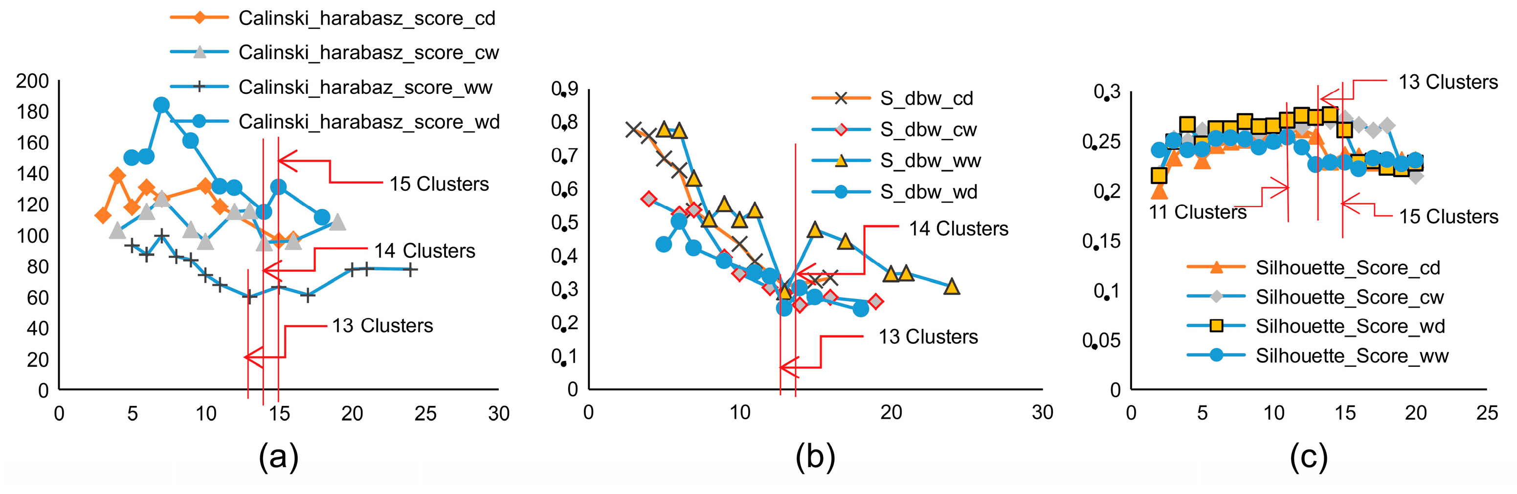
3.1.4. Optimal Clustering and Climate zone Formation

In this step, the optimal CN of stations for each season is identified. Optimal clustering validity methods must be employed for the real grouping of datasets. Comprehensive studies have been performed for the comparative analyses of the cluster validity indices. The silhouette index (S) [66], S Dbw index (S Dbw) [67] and Calinski–Harabasz index (CH) [68] have been used in this study following the recommendations on these comparative evaluations [67,69].

Using the average of the three values identified through the aforementioned validity indices, the optimal CN was identified. The numbering and identification of stations in each cluster were performed via the truncation of the dendrogram. The truncation (cut-off) bar is kept at the valid maximum Euclidian distance corresponding to the validated value of CN [20]. This was performed using a supervised learning algorithm in scikit-learn [53].

Silhouette Score

The silhouette score method [66] is employed in the analysis to obtain the optimum CN. The silhouette score is the mean of the distance between clusters. In this study, the silhouette score yielded a maximum of 14 clusters for climate zoning for all seasons. The CN corresponding to the maximum silhouette score is the basis for the decision. The Silhouette score (S) is obtained as

$$S=\frac{1}{CN}{{\displaystyle \sum }}_i\frac{1}{n_i}{{\displaystyle \sum }}_{r\in C_i}\frac{b\left(r\right)-a\left(r\right)}{\max \left[b\left(r\right),a\left(r\right)\right]}$$

(1)

and

$$a\left(r\right)=\frac{1}{n_i-1}{{\displaystyle \sum }}_{s\in C_i,s\ne r}d\left(r,s\right),b\left(r\right)=mi{n}_{j,j\ne i}\left[\frac{1}{n_j}{{\displaystyle \sum }}_{y\in C_j}d\left(r,s\right)]\right]$$

(2)

where the number of clusters is denoted by CN; C_i represents the ith cluster; n_i represents the number of objects in C_i; c_i denotes the center of C_i; and d(r,s) is the distance between r and s [66].

S Dbw Validity Index

S Dbw considers the inter-cluster density to calculate inter-cluster separation [67]. One of the densities of each cluster pair must be greater than the midpoint density for the cluster centers. This index is the summation of the scatter in the clusters and the density between the clusters. Previous studies have investigated the validation properties of different cluster validity indices using synthetic experimental data [70]. They conclude that S Dbw performed best concerning the aspects of noise, monotonicity, density, skewed distribution and sub-clusters. Equations (3)–(5) can be used to calculate the density between clusters, the scatter in the clusters and the S Dbw, respectively:

$$Dens\_bw\left(CN\right)=\frac{1}{CN\left(CN-1\right)}{\displaystyle \sum }_{i=1}^{CN}\left[{\displaystyle \sum }_{j=1,i\ne j}^{CN}\frac{{{\displaystyle \sum }}_{x_i\in C_i{{\displaystyle \cup }}^{}{C}_j}f\left(x_i,u_{ij}\right)}{\max \left\{{{\displaystyle \sum }}_{xϵC_i}f\left(x,c_i\right),{{\displaystyle \sum }}_{xϵC_j}f\left(x,c_j\right)\right\}}\right]$$

(3)

$$Scat\left(CN\right)=\frac{1}{CN}{\displaystyle \sum }_{i=1}^{CN}\frac{\Vert \sigma \left(C_i\right)\Vert }{\Vert \sigma \left(D\right)\Vert },Dis\left(CN\right)=\frac{ma{x}_{i,j }d\left(c_i,c_j\right)}{mi{n}_{i,j }d\left(c_i,c_j\right)}{\displaystyle \sum }_{i=1}^{CN}{\left({\displaystyle \sum }_{j=1}^{CN}d\left(c_i,c_j\right)\right)}^{-1}$$

(4)

$$S\_Dbw=Scat\left(CN\right) +Dens\_bw\left(CN\right),$$

(5)

where D is the dataset; CN is the number of clusters; σ(C_i) is the variance vector of C_i, σ(D) is the variance in the dataset, (c_i, c_j) is the distance between c_i and c_j and $\Vert x\Vert ={\left(x^{T}x\right)}^{1/2}$.

Calinski–Harabasz Index

This cluster validation scheme depends on the average of the cluster sum of squares and the average of the sum of squares within clusters and is known as CH [68]. It is obtained by formula as shown in Equation (6)

$$CH=\frac{{{\displaystyle \sum }}_i{n}_i{d}^2\left(c_i,c\right)/\left(CN-1\right)}{{{\displaystyle \sum }}_i{{\displaystyle \sum }}_{x\in C_i}{d}^2\left(x,c_i\right)/\left(n-CN\right)}.$$

(6)

Here, n represents the number of points/objects in D, c denotes the center of D and d (x, c_i) denotes the distance between x and c_i.

3.1.5. Climate Zone Polygon Formation

The realistic partition of climatic stations for coherent climate regions is a result of this method. The delineation of these regions depends on the similarity among the statistical climate characteristics of all the stations present in a region.

The clusters of stations for every season were plotted using the ArcGIS (Environmental Systems Research Institute, CA, USA) interface. After the identification of a group of stations in the different clusters, approximate cluster boundaries were drawn on the maps using the Arc-map tool to enable a clearer presentation.

3.2. GCM Selection

The criteria used to select the GCMs are the availability of the latest generation of GCMs, good spatial resolution, past performance of GCM to replicate the historical data and the representativeness of the GCM for a wide range of climatic variable (precipitation) projections [7]. The most commonly adopted criteria are the assessment and selection of GCMs based on their capability to simulate the historical and present climate, which have been adopted by numerous studies [8,9,10]. An efficient and sensible selection of GCMs is required to generate reliable and diverse meteorological inputs for the impact models. Most previous studies show that a past performance assessment is among the most effective methods for the selection of GCMs, as the GCMs thus selected can be better predictors of future climatic conditions [31].

Several selection methods have been reported in the literature. Aghakhani et al. [71] extracted GCM data at four points in the vicinity of observation stations and performed a comparative analysis between the GCM and the observed data. They used the averages of the time-series data at each station for their analysis. Xuan et al. [72] selected GCMs using an average of the climate parameters for the entire study area in the Zhejiang Province of Southeast China. Najeebullah et al. [32] ranked the GCMs at every grid point after re-gridding the GCM data at the same spatial resolution, comparing the data with the gridded data product of the Asian Precipitation - Highly-Resolved Observational Data Integration Towards Evaluation (APHRODITE) for GCM performance evaluations in all of Pakistan. When comparing the best GCM with the highly ranked GCM at each grid station, they found a significant difference between the two with respect to precipitation. Maxino et al. [15] analyzed the climate models from the Fourth Assessment Report (AR4) of the United Nations Intergovernmental Panel on Climate Change (IPCC) for two regions in the Murray Darling Basin, divided based on rainfall classification. For different climate variables, they demonstrated that the models that are flawed in one region may be better for another region; model selection should be area specific. They calculated the skill scores associated with the different climate models in the study region. Lutz et al. [22] averaged the climate data over 2.5° × 2.5° grid cells in three river basins (i.e., the Indus, Brahmaputra and the Ganges) and presented their model with the selected GCMs. Latif et al. [73] also suggested certain Coupled Modelled Intercomparison Project 5 (CMIP5) GCMs after evaluating their performance using seasonal rainfall spatial correlations in the Indo-Pak region. Ahmed et al. [7] evaluated the spatial accuracy of the CMIP5 GCMs using different spatial metrics for all of Pakistan. They performed the analysis after re-gridding the GCM data into a 2° × 2° grid size. Srinivasa et al. [31] ranked the GCMs for the maximum and minimum temperatures across India. This framework comprised the evaluation of GCM suitability at every grid point and then ranking the GCMs using compromised programming.

In the present study, after defining the clusters of stations with homogeneous precipitation, one representative station was selected in every climate zone, using quota sampling [61]. The selection of the representative station was done based on the average climate signal climate signals (Component Scores) in a respective climate zone. The comparative analysis of GCMs data and APHRODITE data at the representative station of each climate zone was accomplished using the coefficient of determination (R²).

A reduced correlation existed within the daily outputs of the GCMs and the in situ data. However, better correlations were obtained when seasonal data in the GCMs were compared with the seasonal observation data. Therefore, using the seasonal data, the correlations between the GCM data and observed gridded data were evaluated at each representative station in the respective climate zone.

3.3. Validation of Selected GCMs

This is the important step of comparative analysis of the climatic data generated through the present selection method of the GCMs and the contemporary method of sampling through simple mean based multi-model Ensemble (MME) data. The KS test [74], a nonparametric test, was used to determine the validity of the selected GCM by detecting the changes in the distribution of the two datasets (dataset generated through present selection method and simple mean based MME data) with the APHRODITE. For every grid station, the observational precipitation data (APHRODITE), selected GCM simulated data of precipitation and multi-model ensemble(MME) mean daily precipitation data of all the 21 GCMs of NASA Earth Exchange Global Daily Downscaled Projections (NEX-GDDP) CMIP5 for the same baseline period from 1970–2005 were used in this test.

3.3.1. Seasonal Data Sampling

The daily precipitation data of the selected GCM, corresponding to each homogeneous climate zone, were seasonally resampled for every grid station (i.e., the grid station within each grid cell). The multi-model ensemble mean data were generated by resampling the data as the average of the GCM daily precipitation data at every grid station.

3.3.2. Kolmogorov–Smirnov Test

In this study, the KS test stats were derived as the highest vertical difference between the two cumulative distribution functions (CDFs) of a time series data. For CDF of APHRODITE data ø_n(x) and the CDF of the selected GCM or MME mean at a grid station ø (x), the KS test statistics were obtained as given in Equations (7) and (8).

$$S_n=su{p}_x\left|{ø}_n\left(x\right)-ø\left(x\right)\right|,$$

(7)

where

$${ø}_n\left(x\right)=\frac{1}{n}{{\displaystyle \sum }}_{i=1}^n{I}_{x_i\le x}.$$

(8)

Here, $su{p}_x$ is the upper bound of the set of distances. The indicator function is represented by $I_{x_i\le x}$ (If $x_i\le x$, $I_{x_i\le x}$ equal to 1 or if $x_i >x{I}_{x_i\le x}$ equal to 0). The null hypothesis of a similar distribution is rejected if $S_n$ $\ge$ 0.05 significance level. The KS test was applied at every grid station using scikit-learn.

3.4. Selection of Forcing Scenarios

Four climate forcing scenarios are commonly used in climate research for climate simulation studies on both long term and short term scales. There are four common Representative Concentration Pathways (RCPs)—RCP 2.6 is a mitigation scenario; RCP 4.5 and RCP 6.0 are scenarios of medium stabilization and RCP 8.5 is a high baseline emissions scenario [75]. We did not include RCP 2.6 for the ensemble of climate models, as it is not considered a realistic or practical scenario necessary to promote adaptation planning. These rest of the three scenarios represent the complete extent of radiative forcing. In this study, we used the RCP 4.5 and RCP 8.5. The same framework applies to other forcing scenarios [22].

Extraction of Selected GCMs Data for RCP 4.5 and 8.5

The daily precipitation data for the selected GCM in the specific climate zone for the projected period from 2006–2099, as well as forcing scenarios RCP 4.5 and 8.5, were sampled for all seasons at every grid station.

3.5. Climate Change Projections and Trend Detection

The highly correlated GCMs, which can replicate the gridded dataset of seasonal precipitation for the period from 1970–2005, were selected in each climate zone for use in the future predictions of precipitation change trends in RCP 4.5 and RCP 8.5. The precipitation change trends were detected using the Mann–Kendall (MK) test during the projected period (2006–2099). The trend was quantified by employing Sen’s slope estimator.

3.5.1. Mann-Kendall Test (MK Test)

The MK test [76] was used to evaluate the statistically significant annual seasonal trends in the long term precipitation data. The “no trend” in precipitation with time is assumed in the null hypothesis (H_o) of the test and vice versa for the alternative hypothesis (H_a). The Equations (9)–(12) show the test stats T of the MK test.

$$T={\displaystyle \sum }_{i=1}^{n-1}{\displaystyle \sum }_{j=i+1}^{n}sig\left(D_j-D_i\right)$$

(9)

$$sgn\left(D_j-D_i\right)=\{\begin{array}{c}+1 if \left(D_j-D_i\right)>0\\ 0 if \left(D_j-D_i\right)=0 \\ -1 if \left(D_j-D_i\right)<0\end{array}$$

(10)

$$\sigma \left(T\right)=\frac{1}{18}\left[n\left(n-1\right)\left(2n+5\right)-{\displaystyle \sum }_{p=1}^q{t}_p\left(t_p-1\right)\left(2t_p+5\right)\right]$$

(11)

$$Z=\{\begin{array}{c}\frac{T-1}{\sqrt{\sigma \left(T\right)}} if T>0\\ 0 if T=0\\ \frac{T-1}{\sqrt{\sigma \left(T\right)}} if T<0 \end{array},$$

(12)

where D_i and D_j are the consecutive time-series observations, which are organized chronologically for the length of data (n); t_p represents the data points number for the pth value in a tied group; and q denotes the total number of tied groups σ is the variance. An upward time series trend is represented by a positive Z value and vice versa for the negative trend. If $\left|Z\right|>Z_{1-\alpha /2}$, the null hypothesis (H_o) is rejected which is indicative of a statistically significant trend. The critical value of $Z_{1-\alpha /2}$ is assumed at the p-value of 0.05.

3.5.2. Sen’s Slope Evaluation

The Python module was applied to obtain the slope of the trend, if exists, according to Sen’s method [77]. According to the method, linear slope sets can be estimated as shown in Equation (13).

$$T_i=\frac{D_j- D_k}{j-k}\mathrm{for}(1\le i<j\le \mathrm{n}),$$

(13)

where Ti is the slope, D_j and D_k are the variables at j and k time steps, respectively and n represents the data points number. Sen’s slope is estimated as the median of all slopes.

4. Results and Discussion

Taking the spatiotemporal average [22,25,73] of the climate dataset at all the grid points of the area at different temporal scales (daily, seasonal or annual) or using various spatial metrics on the results of the individual grid points [21,31,32] are the conventional methods used for the selection of GCMs. However, these methods do not address the spatial coherence of the climate variability patterns in the study area. This poses uncertainty in using these conventional methods. Several studies support the association between atmospheric covariates and precipitation. In GCMs, these atmospheric covariates are the input variables. To address the uncertainty arising from the input variables of the GCMs, it is imperative to assess the GCM performance in reproducing the regional climate pattern. These results show that the climate variability pattern of the study area is spatially heterogeneous in all seasons and a single or an ensemble of GCMs may not represent this spatial climatic heterogeneity. Therefore, we classified/ regionalized the large study in several climate zones founded on the climate variability patterns similarity and the selection of a GCM should be done separately in each of the homogeneous climate zones.

This section presents the detailed results along with the discussion. The results have been visualized using ArcGIS. This software is based on the integration of different machine learning techniques. Section 4.1 describes the results of the analyses performed for the development of climate zones. Section 4.2 shows the results of the GCM selection procedure and Section 4.3 is related to the validation of the method used for the GCM selection. Section 4.4 described the results of the MK test of trend detection and Sen’s slope estimation. These tests determined the precipitation change trend projections for the period of 2006 to 2099.

4.1. Climate Zones

The Principal Component Analysis (PCA) performed as the first step in climate zoning provided the details of the climate change pattern in the entire study area. A statistically significant climate pattern heterogeneity was observed in the region when PCA was performed on a seasonal basis.

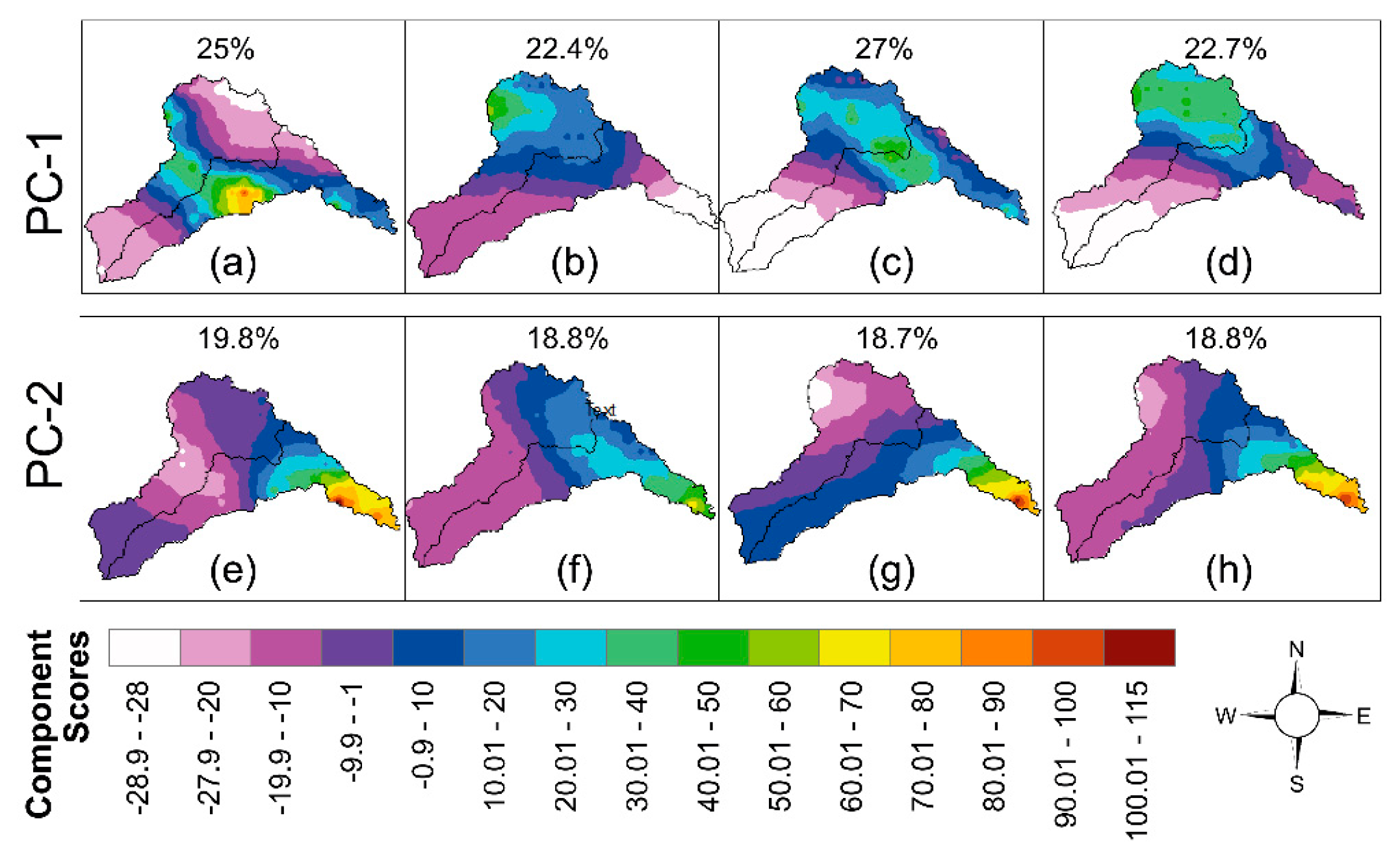
4.1.1. Principal Component Analysis

The application of the Principal Component Analysis (PCA) was performed on the daily precipitation series data from APHRODITE on a network of 138 stations distributed across the Jhelum and Chenab river basins. This first led to 20 primary and physically significant principle components (PCs), which collectively explained approximately 95% of the total variability in the precipitation throughout the study area. These were retained for the cluster analysis. Scree Plot is shown in Figure 4. The PCA algorithm produced the scree plots, allowing us to select the number of PCs for the cluster analysis. For the warm-wet season, 20 PCs present 95% of the data variance from the station network (Figure 4a). For the cold-dry season, 20 PCs present 94% of the variance in the data from the station network (Figure 4b). For the cold-wet season, 20 PCs explained 95% of the variance in the data from the station network (Figure 4c). For the warm-dry season, 20 PCs explained 95% of the variance in the data from the station network (Figure 4d). The spatial distribution of the component scores is shown in Figure 5, for the first two PCs, explaining the highest percentage of variance in the data.

These two PCs cumulatively produced variance of 44.8% in the warm-wet season, 41.2% in the cold-dry season, 45.7% in the cold-wet season and 41.5% in the warm-dry season. For the component scores, the first PC for the warm-wet season, as shown in Figure 5a (with 25% of the explained variance), has high negative scores in the north and southwest of the study region and medium-high positive signals in the central region. Stronger positive and negative signals exhibit an affinity of higher variation in the precipitation amount, while weaker scores indicate low variability. The second PC for the warm-wet season, as shown in Figure 5e (with 19.8% of the explained variance), has mostly positive component scores in the southeast, except for medium and strong negative signals in several southeast and central regions, respectively. In the cold-dry season, we observe higher negative variability in the southwest based on PC1, as shown in Figure 5b and in small areas of the southeast. Strong positive signals were detected in the northwest area of the study region. For PC2, high positive component scores were observed in the southeast, as shown in Figure 5f (with 18.8% of the explained variance), whereas strong negative scores occurred in the southwest area. In the cold-wet season, the variability in the precipitation amount was high in the southwest region for PC1 (with 27% of the explained variance in the data), as shown in Figure 5c and high positive signals in the southeast and central areas of the region. For PC2, cold-wet season (with 18.7% of the explained variance), shown in Figure 5g, had strong positive scores in the southeast area of the region but medium to high negative scores in the rest of the study area. In the warm-dry season, high variability was observed in the precipitation in the northern and southwest regions of the area for the PC1 component score (with 22.7% of the explained variance), as shown in Figure 5d. The PC2 had high positive variability in the southwest and medium negative signals in the rest of the region, as shown in Figure 5h. The first two PCs were noted to explain a significant variability for the precipitation data in all seasons.

4.1.2. Agglomerative Hierarchical Clustering (AHC)

We then identified all the potentially homogeneous regions inside the study area. The extent of the homogeneity in these homogeneous regions was identified using different cluster validity indices. The first 20 PCs were employed in the AHC analysis. These PCs were obtained in the previous step using the Python scikit module. The validity of different site/station clusters was evaluated by performing the silhouette score, CH and S Dbw tests. Figure 6 summarizes the cluster validation results. The machine learning algorithms for the cluster validity were run repetitively using different input values for the maximum Euclidean distance, followed by a comparison of the resulting clusters to obtain their validity. According to the results, the optimized partitioning of the data based on the CH Test was investigated while the lowest scores were estimated corresponding to clusters 13, 15, 14 and 14 for the warm-wet, cold-dry, cold-wet and warm-dry seasons, respectively, as shown in Figure 6a. The partitioning based on the S Dbw test suggests that optimized clustering can be performed when the data is partitioned into clusters 13, 13, 14 and 13 for the warm-wet, cold-dry, cold-wet and warm-dry seasons, respectively, as shown in Figure 6b. These clusters were selected based on the lowest S Dbw scores. The partitioning of data into clusters 11, 15, 13 and 13 corresponds to the highest silhouette test scores for the warm-wet, cold-dry, cold-wet and warm-dry seasons, respectively, as shown in Figure 6c.

Based on Figure 6, all validity measures agree with the same number of clusters. Therefore, based on the recommendations of previous studies [70], we partitioned the stations for optimized clustering as clusters 13, 13, 14 and 13 for the warm-wet, cold-dry, cold-wet and warm-dry seasons, respectively. The members/stations in different clusters were obtained via the truncation of the dendrogram at the Euclidean distances that correspond to the optimized clusters. The dendrograms were obtained from the AHC of the selected PCs. The maximum Euclidean distances were identified as corresponding to the proposed cluster numbers, where Figure 7 shows the cut-off/truncation bars for each season. Based on this truncation, we identified the groups of stations/sites in each cluster. Figure 7 shows the dendrograms that present the cluster trees for all four seasons.

4.1.3. Climate Zones and Reference site

This study reveals useful details on the efficiency of machine learning algorithms when formulating large, homogeneous regions of precipitation for different seasons. Homogeneous precipitation sites were identified based on the validated number of cluster-values. These station clusters were then plotted on a study area map, as shown in Figure 6. All homogeneous regions are differentiated by different colors to show the general spatial patterns associated with precipitation, the approximate boundaries are drawn on the maps to allow for a clearer representation. The clusters of stations transformation into different climate zones for all seasons have been shown in Figure 8.

The Jhelum and Chenab river basins are partitioned into clusters 13, 13, 14 and 13 for the warm-wet, cold-dry, cold-wet and warm-dry seasons, respectively, based on the analysis. There were three outliers in the clusters of the warm-wet season, one outlier in the clusters of the cold-dry season, one outlier in the cold-wet and one outlier in the warm-dry season. After merging the outliers with the neighboring clusters, the final demarcations of the basins were mapped for every season. The basins are finally classified into 10, 12, 13 and 13 climate zones for warm-wet, cold-dry, cold-wet and warm-dry seasons. The reference station was identified in each climate zone for the selection of the best-correlated GCM, using the past performance analysis of the GCM at the reference station in each climate zone.

4.2. GCM Selection

We investigated the capabilities of 21 CMIP5 GCMs to reconstruct the highly resolved observation data for precipitation and, using Pearson correlation analysis, identified the most correlated GCMs for a dependable climate projection in a climate zone. The GCMs were selected in every climate zone of the study area using the GCM and APHRODITE seasonal precipitation data at the reference station. The reference stations in every climate zone for every season have been shown in Figure 8. These selected GCMs were then used for the projections of changes in the precipitation trends at every grid point throughout the respective zone in the river basins. Figure 9 shows the spatial distribution of the highly correlated GCMs in each climate zone. For the warm-wet season, we selected the BNU-ESM, MIROC5, CESM, IPSL-CM5A-MR and GFDL-ESM2G GCMs. For the cold-dry season, we selected the CCSM4, MIROC-ESM, IPSL-CM5A-LR, MIROC5 and MPI-ESM-LR GCMs. For the cold-wet season, we selected the MRI-CGCM3, MIROC-ESM, NorESMI, CESM, IPSL-CM5A-MR and GFDL-ESM2G GCMs. For the warm-dry season, we selected the IPSL-CM5A-MR, BNU-ESM, GFDL-CM3, bcc-CSM1-1, inmcm4 and GFDL-CM3 GCMs. The description of the aforementioned GCMs can be checked from the Table S1 in supplementary documents.

4.3. Validation of Selected GCMs

The selected GCMs and simple mean of MME (21 GCMs) daily precipitation data at every grid station were resampled for the seasonal cycles. The KS test was applied to every grid station and the data distribution was compared with the APHRODITE data distribution. p-values < 0.05 demarcate between the null and alternative hypotheses. When the p-value < 0.05, the similar distribution hypothesis is rejected and vice versa. Figure 10 shows the spatial distribution of the p-value for the KS test. The result shows that the selected GCMs present a higher degree of similarity in the daily seasonal distribution to the APHRODITE distribution as compared with the simple mean of MME distribution. The results show that 45% of the time-series distribution of the selected GCMs’ datasets did not fall in the rejection zone (when α = 5%), on the other hand, when using the datasets of simple mean MME, 28% of the datasets did not fall in the rejection zone for the warm-wet season. 76% of the time-series distribution of the datasets of the selected GCMs did not fall in the rejection zone (when α = 5%) for the cold-dry season, whereas only 55% of the datasets were not in the rejection zone when using the datasets of simple mean MME. For the cold-wet season, 76% of the time-series distribution of the selected GCMs’ datasets did not fall in the rejection zone (when α = 5%), whereas 0% of the datasets were not in the rejection zone when the simple mean MME was tested. For the warm-dry season, 73% of the time-series distribution of the selected GCMs’ datasets did not fall in the rejection zone (when α = 5%), whereas only traces of 10% of the datasets were not in the rejection zone when the simple mean MME was tested. The results validated the GCM selection procedure when assessed against past performance.

4.4. Seasonal Precipitation Trend Projection

The significance of seasonal precipitation trends for the period of 2006–2099, as detected by the MK trend detection test, for forcing scenarios RCP 4.5 and 8.5, are presented in Figure 11. The distribution of p-value spatially for the MK test has been presented. Spatial patterns of the estimated Sen’s slope exhibit negative and positive slopes for the trends in different seasons, as shown in Figure 12. The significance of the trends was identified via the MK test of trend detection, as shown in Figure 11. For the warm-wet season, with the RCP 4.5 forcing scenario (refer to Figure 12a), 28% of the total study region yielded very strong and 5% of the total study region yielded strong evidence for decreasing precipitation at values of 2.2–3.29 mm yr⁻¹ over the central and northwest of the area. For RCP 4.5, 67% of the region showed no or weak decreasing trends. However, for the RCP 8.5 (Figure 12e), weak evidence for increasing trends was detected in the central and southeast region at 0.5–2 mm yr⁻¹, except for certain areas in the central to western regions, where we detected a non-significant decreasing trend, with a slope of 1–3.29 mm yr⁻¹. Figure 11 depicts the p-values for the MK trend detection, which shows significant and non-significant trends.

For the cold-dry season and RCP 4.5 (Figure 12b), nearly all the regions of the study area had weak, increasing trends with Sen’s slopes of 0–0.5 mm yr⁻¹, which are not significant, as depicted in Figure 11. On the other hand, for RCP 8.5 (Figure 12f), weak decreasing trends were detected in the central and southwest regions and certain areas of the southeast, with Sen’s slopes of 0.2 mm yr⁻¹. Here, 80% of the total area had weak evidence of increasing trends at 0.5–1.5 mm/season/year.

For the cold-wet season for the RCP 4.5 (Figure 12c), the weak decreasing trend, with Sen’s slopes of 0.2–0.5 mm yr⁻¹, was detected in the central and southwest parts of the area. High and weak increasing trends were detected in the northwest and southeast parts of the area, respectively. The positive slope varies between 0.5 and 2 mm yr⁻¹.

For the cold-wet season in the RCP 8.5 (Figure 12g), a non-significant decreasing trend was detected with Sen’s slopes varying between 0.5 and 0.2 mm yr⁻¹ in the central area, whereas in other regions, a weak, increasing trend was detected with slopes varying between 0.5 and 2 mm yr⁻¹.

Unlike for the warm-dry season and RCP 4.5 (Figure 12d), there is strong evidence for an increase in the precipitation for the whole study area with p-values from the MK trend detection at less than 0.05 for nearly the entire study area, with the Sen’s slope indicating an increase in the precipitation rate with values varying between 1.5 and 3.5 mm yr⁻¹. The same is the case for RCP 8.5 in the warm-dry season based on strong evidence of an increase in the precipitation throughout the entire area, with Sen’s slope values varying between 1.5 and 3.5 mm yr⁻¹ (Figure 12h). Figure 11 shows the p-values for the MK test for the best-correlated models (2006–2099) for RCPs 4.5 and 8.5.

5. Conclusions

Previous studies have not currently arrived at a consensus on a universally accepted method and criteria used for GCM selection [14,78]. Studies continue to investigate the methods, whether dynamic or statistical, to reduce the uncertainty in predicting climate change impacts. Intending to reduce the uncertainty, we presented a novel and flexible framework for the selection of GCMs in homogeneous climatic zones, which are based on daily seasonal precipitation data statistics spanning the baseline/historical period (1970–2005) for the Jhelum and Chenab river basin study areas. The GCM selected in each of the climate zones of every season can reproduce the climate distribution patterns in the study area. This has been proved by comparatively analyzing the precipitation data sets of GCMs selected and the simple composite mean of the ensemble of the 21 CMIP5 GCMs. Using these homogeneous precipitation regions, we suggest a different approach for selecting the GCMs. The GCMs were selected based on prior performance and compared with the highly resolved and gridded APHRODITE data. The GCM selection was validated for its performance to emulate the spatial precipitation patterns during the baseline period (1970–2005) for the study region. We sampled the daily precipitation data for the projected period using the selected GCM. The trends in the precipitation variability, based on the MK trend detection statistics, show that the regions in the Jhelum and Chenab river basins have negative, positive and no trends from 2006 to 2099.

The Jhelum and Chenab river basins are scarcely gauged regions; hence, the APHRODITE gridded datasets were used in this study because this type of climate zoning requires a dense network of climate observation stations. Numerous previous studies have verified the reliability of the APHRODITE data in this region [22,40]. However, at high altitudes, the deviation between the gridded data and in situ observations is more than that of flat regions due to a reduced number of gauging stations in mountainous areas, which poses a challenge to precise interpolation [79]. Uncertainties in the forcing datasets persist due to the scarcity of gauging stations in high elevation zones. Furthermore, gauging stations in valleys cannot represent peripheral higher elevation zones due to the high vertical lapse rate of precipitation [41]. Currently, there is no consensus among the climate research community regarding the methods of bias correction for high elevation areas. The comparative analysis shows that the APHRODITE correlates well with the observed dataset of some gauging stations at high altitudes, leading to the assumption of having sufficient accuracy for the regionalization process. Nevertheless, this regionalization framework is equally applicable to other datasets having comparatively higher resolution and accuracy.

All the analyses were conducted using the Python programming language, which is known to be powerful in machine learning. Several machine learning modules from the scikit-learn library, such as Principal Component Analysis (PCA), Agglomerative Hierarchical Clustering (AHC) and clustering validity indices, correlation coefficient and the KS test, were used in the analysis. All these machine learning algorithms were compiled to develop a program for regionalization and climate change trend detection. The program can be provided to the climate research community to augment decision- and policymaking for water resource planning and management.

Potential forecasts from the GCMs, however, are fundamentally uncertain and decision-makers still find it difficult to understand or use such predictions of climate change. The major cause of this uncertainty in the assessments derives from the inherent uncertainties in GCM outputs [80,81,82,83]. Based on the results and interpretations presented in this study, we can draw the following conclusions:

1)

Due to its highly volatile hydroclimatic conditions, this area of Pakistan poses major scientific challenges; hence, investigations require complex methods. Multivariate techniques, such as PCA and Agglomerative Hierarchical Clustering (AHC) algorithms, are used to develop decisive precipitation statistics and delineate homogeneous precipitation regions, respectively. The entire study area was divided into 13 homogeneous precipitation regions for the warm-wet season, 13 homogeneous precipitation regions for the cold-dry season, 14 homogeneous precipitation regions for the cold-wet season and 13 homogeneous precipitation regions for the warm-dry season. The reference station, which is representative of the respective homogeneous precipitation regions, was obtained in each homogeneous precipitation region for GCM selection. Seasonal rainfall characteristics were incorporated to define the homogeneous climate regions to design the climate zones in the river basins of Pakistan. Representative rainfall station/grid points were selected in each climate zone for the climate change impact assessment. This study provides an objective demarcation structure for homogeneous precipitation regions based on the statistical characteristics of seasonal precipitation.

2)

The best-correlated GCM was identified in each climate zone in the Jhelum and Chenab river basins, followed by data extraction. This selection was validated and compared spatially with the KS test. Two schemes of the daily precipitation data were derived: (1) the precipitation data sampled from the selected GCMs based on this framework and (2) the precipitation data from the MME mean (21 models of the CMIP5 mean). The KS test was used to measure the compatibility of the observed data with data from scheme 1 and then the data from scheme 2. The results clearly show the improved performance of the present framework for the selected GCMs compared with the conventional method involving the equally weighted means of all the available GCMs.

3)

The precipitation pattern can represent the climatic dynamics because the atmospheric circulation covariates have a strong correlation with the precipitation patterns in the region [2]. The daily projected precipitation data (2006–2099), synthesized for the regions of the Jhelum and Chenab river basins, are publicly available. The creation of homogeneous climatic zones accommodates a deeper understanding of the dynamic spatio-temporal precipitation variability over a given region. Infrastructure development and climate forecasting are based on effective regionalization using reliable estimates of climate variables. The region should be conditionally considered as climatically homogeneous to proceed with the selection of GCMs for the climate change impact assessments.

4)

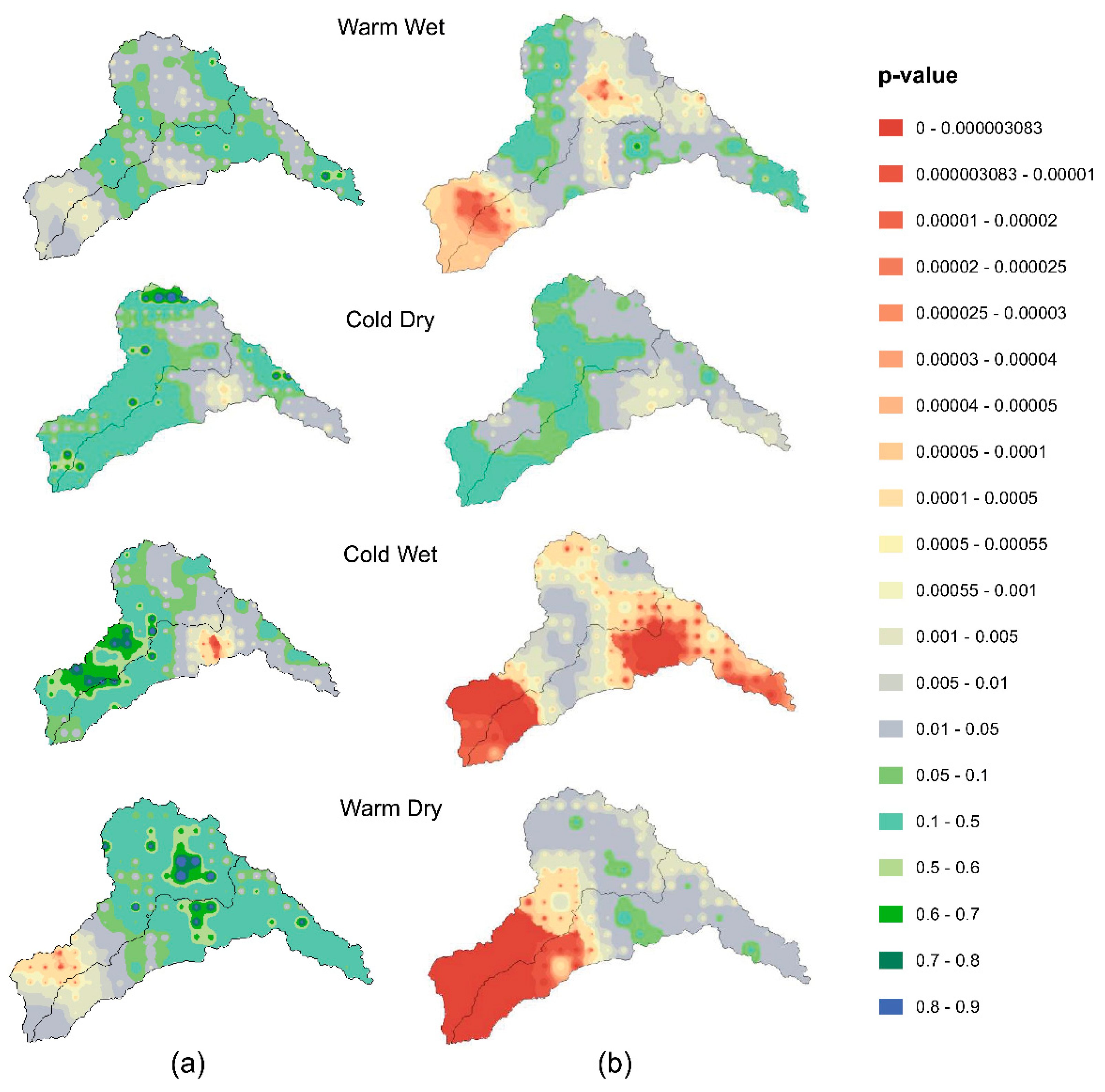
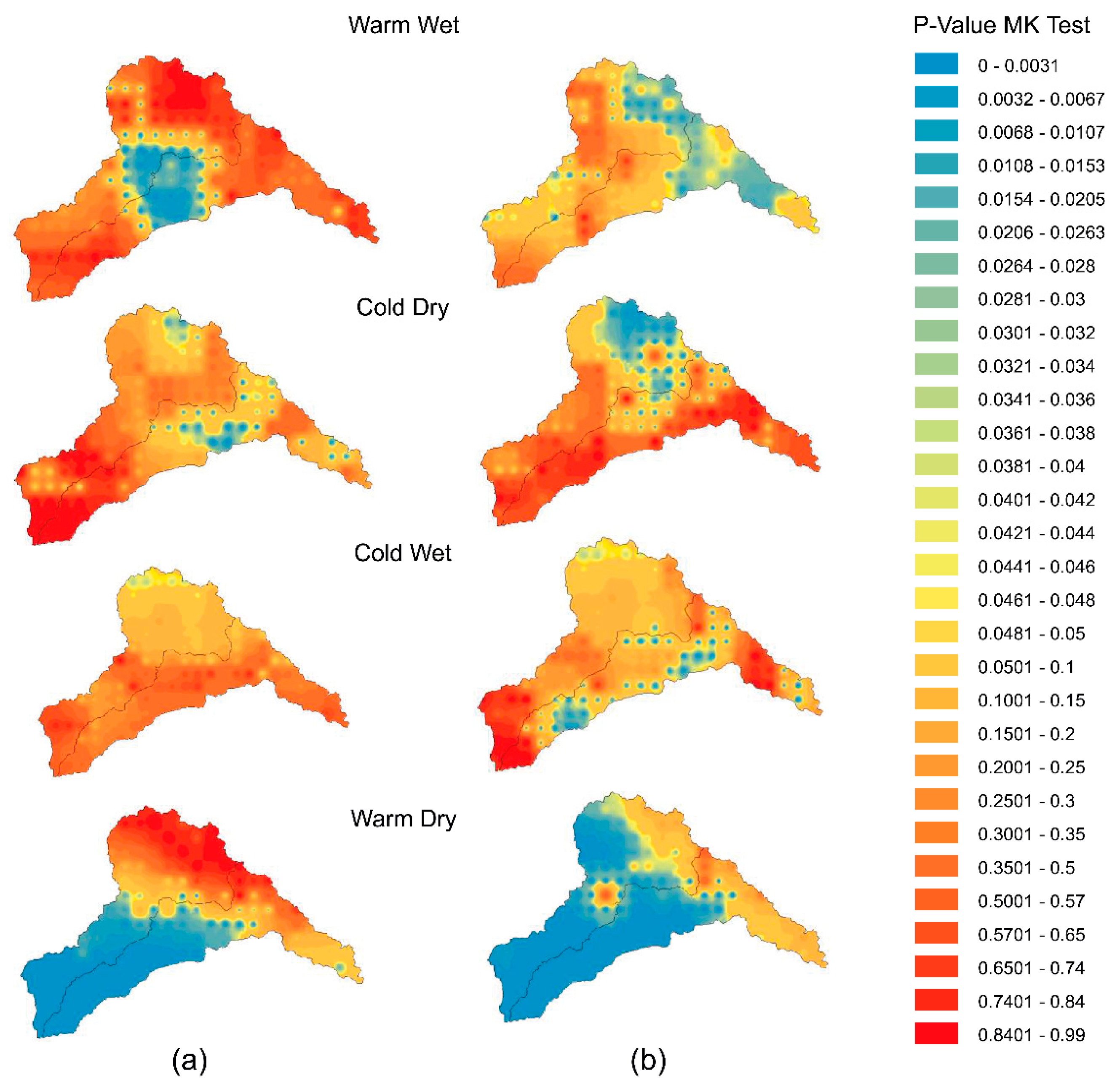
The projections of the changes in the precipitation trends were presented based on two scenarios, that is, RCP 4.5 and RCP 8.5. For the RCP 4.5, a significant positive precipitation trend was observed for the warm-dry season, while insignificant positive trends were observed for the cold dry and cold wet seasons. A negative precipitation trend was observed throughout the entire study area, in which 40% of the area had a significant negative trend for the warm-wet season. For the RCP 8.5, the warm-dry season again exhibited a significant positive precipitation trend, whereas insignificant positive trends were observed for the warm-wet, cold-dry and cold-wet seasons. The effect of the precipitation change trends may have greater implications on water resources and its management. This unique study provides spatial changes in patterns, as well as temporal changes. Strong increasing and decreasing signals occurred during the warm-dry season for both scenarios in the river basins. Precipitation trends were detected within this framework, which were mapped spatially across the entire study region.

5)

Future studies should redefine the homogeneous precipitation region and change detection using the projected data to obtain the hydrological response in a basin using this projected input data for the rainfall. The same framework, with a set of machine learning modules, can be employed to select and detect precipitation trends using the next generation of GCMs. More than 125 years of precipitation data of daily scale, were used for the analyses in this study, which depicts the strength of machine learning.

There is extensive literature available, addressing the uncertainties in climate projections through climate models [5,17]. The uncertainty in predicting the near future day to day weather of dynamic chaotic weather systems has been discussed by meteorologist Edward N Lorenz [16], in which he emphasized the theory of chaos, that is, the importance of the sensitivity of initial state simulation and parametrization of a model for plausible weather forecast. The knowledge of the precise initial state of the weather conditions is essential for the robust whether forecast, furthermore, it is also useful to predict the climate having initial conditions of weather. However, the predictability of the weather is limited to few days due to the reason of atmospheric dynamics. Weather patterns are affected by atmospheric oscillations such as El Nino and La Nina. Climate projections are done using the heat energy changes on Earth’s surface and the changes in greenhouse gas emissions in the atmosphere. The projections of these changes to eventually project the climate is significantly easier than the weather forecasting of a week. To summaries, long term changes in atmospheric composition are significantly more predictable than the short term weather forecast [84].

The sources of confidence in future projections by the models are their physical basis and their performance in simulating the past/historical climate. According to IPCC, the models have been proven as important tools to project the future climate [84]. Their performance in representing large scale climate features are extensively evaluated through the comparative analysis of its simulations with the observations and they have been used to predict the ancient climate such as the warm Holocene period, the last glacial maximum and the last ice age [84].

The paper is envisioned to provide a framework that can easily be replicated to project the climate change trends for an area by utilizing the stochastic analysis strengths of machine learning and the available observed and GCMs’ data. It tends to be an important reference to those who are working on impact modeling. However, it does not aim to discuss the dynamic processes and associated uncertainties present in all GCMs. These are presented in the literature and their simulation outputs have been used in the analysis. To gain a higher confidence level, the end-users of the present framework are suggested to use large ensemble of GCMs while selecting a suitable model in each zone of the study area. The codes prepared in this study are provided upon request.

Further studies are required to analyze the seasonal climate shift and how accurately the GCM outputs can project the present climatic zones, which are delineated based on the observed gridded historical data.

References

1. Jamro, S.; Channa, F.N.; Dars, G.H.; Ansari, K.; Krakauer, N.Y. Exploring the Evolution of Drought Characteristics in Balochistan, Pakistan. Appl. Sci. 2020, 10, 913. [Google Scholar] [CrossRef] [Green Version]
2. Asong, Z.E.; Khaliq, M.N.; Wheater, H.S. Regionalization of Precipitation Characteristics in the Canadian Prairie Provinces Using Large-scale Atmospheric Covariates and Geophysical Attributes. Stoch. Environ. Res. Risk Assess. 2015, 29, 875–892. [Google Scholar] [CrossRef]
3. Christensen, J.; Kanikicharla, K.; Aldrian, E.; An, S.-I.; Fonseca, I.; Castro, M.; Dong, W.; Goswami, P.; Hall, A.; Kanyanga, J.K.; et al. Climate Phenomena and Their Relevance for Future Regional Climate Change; IPCC: Geneva, Switzerland, 2013; pp. 1–92. [Google Scholar]
4. McSweeney, C.F.; Jones, R.G.; Lee, R.W.; Rowell, D.P. Selecting CMIP5 GCMs for downscaling over multiple regions. Clim. Dyn. 2015, 44, 3237–3260. [Google Scholar] [CrossRef] [Green Version]
5. Ahmed, K.; Shahid, S.; Chung, E.-S.; Wang, X.; Harun, S.B. Climate Change Uncertainties in Seasonal Drought Severity-Area-Frequency Curves: Case of Arid Region of Pakistan. J. Hydrol. 2019, 570, 473–485. [Google Scholar] [CrossRef]
6. Wu, C.; Huang, G.; Yu, H.; Chen, Z.; Ma, J. Impact of Climate Change on Reservoir Flood Control in the Upstream Area of the Beijiang River Basin, South China. J. Hydrometeor. 2014, 15, 2203–2218. [Google Scholar] [CrossRef]
7. Ahmed, K.; Sachindra, D.A.; Shahid, S.; Demirel, M.C.; Chung, E.S. Selection of multi-model ensemble of general circulation models for the simulation of precipitation and maximum and minimum temperature based on spatial assessment metrics. Hydrol. Earth Syst. Sci. 2019, 23, 4803–4824. [Google Scholar] [CrossRef] [Green Version]
8. Ismail, H.; Kamal, M.R.; Abdullah, A.F.B.; Jada, D.T.; Sai Hin, L. Modeling Future Streamflow for Adaptive Water Allocation under Climate Change for the Tanjung Karang Rice Irrigation Scheme Malaysia. Appl. Sci. 2020, 10, 4885. [Google Scholar] [CrossRef]
9. Uamusse, M.M.; Tussupova, K.; Persson, K.M. Climate Change Effects on Hydropower in Mozambique. Appl. Sci. 2020, 10, 4842. [Google Scholar] [CrossRef]
10. Touseef, M.; Chen, L.; Masud, T.; Khan, A.; Yang, K.; Shahzad, A.; Wajid Ijaz, M.; Wang, Y. Assessment of the Future Climate Change Projections on Streamflow Hydrology and Water Availability over Upper Xijiang River Basin, China. Appl. Sci. 2020, 10, 3671. [Google Scholar] [CrossRef]
11. Yu, Z.; Man, X.; Duan, L.; Cai, T. Assessments of Impacts of Climate and Forest Change on Water Resources Using SWAT Model in a Subboreal Watershed in Northern Da Hinggan Mountains. Water 2020, 12, 1565. [Google Scholar] [CrossRef]
12. Dikshit, A.; Pradhan, B.; Alamri, A.M. Short-Term Spatio-Temporal Drought Forecasting Using Random Forests Model at New South Wales, Australia. Appl. Sci. 2020, 10, 4254. [Google Scholar] [CrossRef]
13. Zhao, Q.; Ma, X.; Liang, L.; Yao, W. Spatial–Temporal Variation Characteristics of Multiple Meteorological Variables and Vegetation over the Loess Plateau Region. Appl. Sci. 2020, 10, 1000. [Google Scholar] [CrossRef] [Green Version]
14. McMahon, T.A.; Peel, M.C.; Karoly, D.J. Assessment of Precipitation and Temperature Data from CMIP3 Global Climate Models for Hydrologic Simulation. Hydrol. Earth Syst. Sci. 2015, 19, 361–377. [Google Scholar] [CrossRef] [Green Version]
15. Maxino, C.C.; McAvaney, B.J.; Pitman, A.J.; Perkins, S.E. Ranking the AR4 Climate Models over the Murray-Darling Basin Using Simulated Maximum Temperature, Minimum Temperature and Precipitation. Int. J. Climatol. 2008, 28, 1097–1112. [Google Scholar] [CrossRef]
16. Lorenz, E.N. Predictability: A Problem Partly Solved. In Proceedings of the Seminar on Predictability, Shinfield Park, Reading, UK, 4–8 September 1995. [Google Scholar]
17. Hawkins, E.; Sutton, R. The Potential to Narrow Uncertainty in Projections of Regional Precipitation Change. Clim. Dyn. 2011, 37, 407–418. [Google Scholar] [CrossRef]
18. Baker, N.; Taylor, P. A Framework for Evaluating Climate Model Performance Metrics. J. Clim. 2016, 29, 1773–1782. [Google Scholar] [CrossRef]
19. Chhin, R.; Yoden, S. Ranking CMIP5 GCMs for Model Ensemble Selection on Regional Scale: Case Study of the Indochina Region. J. Geophys. Res. Atmos. 2018, 123, 8949–8974. [Google Scholar] [CrossRef]
20. Wilcke, R.A.I.; Bärring, L. Selecting Regional Climate Scenarios for Impact Modelling Studies. Environ. Model. Softw. 2016, 78, 191–201. [Google Scholar] [CrossRef] [Green Version]
21. Salman, S.A.; Shahid, S.; Ismail, T.; Ahmed, K.; Wang, X.-J. Selection of Climate Models for Projection of Spatiotemporal Changes in Temperature of Iraq with Uncertainties. Atmos. Res. 2018, 213, 509–522. [Google Scholar] [CrossRef]
22. Lutz, A.F.; ter Maat, H.W.; Biemans, H.; Shrestha, A.B.; Wester, P.; Immerzeel, W.W. Selecting Representative Climate Models for Climate Change Impact Studies: An Advanced Envelope-Based Selection Approach. Int. J. Climatol. 2016, 36, 3988–4005. [Google Scholar] [CrossRef] [Green Version]
23. Cannon, A.J. Selecting GCM Scenarios that Span the Range of Changes in a Multimodel Ensemble: Application to CMIP5 Climate Extremes Indices. J. Clim. 2015, 28, 1260–1267. [Google Scholar] [CrossRef]
24. Azmat, M.; Qamar, M.U.; Huggel, C.; Hussain, E. Future Climate and Cryosphere Impacts on the Hydrology of a Scarcely Gauged Catchment on the Jhelum River Basin, Northern Pakistan. Sci. Total Environ. 2018, 961–976. [Google Scholar] [CrossRef] [PubMed]
25. Mahmood, R.; Jia, S.; Tripathi, N.K.; Shrestha, S. Precipitation Extended Linear Scaling Method for Correcting GCM Precipitation and Its Evaluation and Implication in the Transboundary Jhelum River Basin. Atmosphere 2018, 9, 160. [Google Scholar] [CrossRef] [Green Version]
26. Kim, J.-B.; So, J.-M.; Bae, D.-H. Global Warming Impacts on Severe Drought Characteristics in Asia Monsoon Region. Water 2020, 12, 1360. [Google Scholar] [CrossRef]
27. Gu, H.; Yu, Z.; Wang, J.; Wang, G.; Yang, T.; Ju, Q.; Yang, C.; Xu, F.; Fan, C. Assessing CMIP5 General Circulation Model Simulations of Precipitation and Temperature over China. Int. J. Climatol. 2015, 35, 2431–2440. [Google Scholar] [CrossRef]
28. Fu, G.; Charles, S.P.; Kirshner, S. Daily Rainfall Projections from General Circulation Models with a Downscaling Nonhomogeneous Hidden Markov Model (NHMM) for South-Eastern Australia. Hydrol. Process. 2013, 27, 3663–3673. [Google Scholar] [CrossRef]
29. Johnson, F.; Sharma, A. Measurement of GCM Skill in Predicting Variables Relevant for Hydroclimatological Assessments. J. Clim. 2009, 22, 4373–4382. [Google Scholar] [CrossRef]
30. Schaeffer, M.; Selten, F.M.; Opsteegh, J.D. Shifts of Means Are Not a Proxy for Changes in Extreme Winter Temperatures in Climate Projections. Clim. Dyn. 2005, 25, 51–63. [Google Scholar] [CrossRef]
31. Srinivasa Raju, K.; Sonali, P.; Nagesh Kumar, D. Ranking of CMIP5-based global climate models for India using compromise programming. Theor. Appl. Climatol. 2017, 128, 563–574. [Google Scholar] [CrossRef]
32. Khan, N.; Shahid, S.; Ahmed, K.; Ismail, T.; Nawaz, N.; Son, M. Performance Assessment of General Circulation Model in Simulating Daily Precipitation and Temperature Using Multiple Gridded Datasets. Water 2018, 10, 1793. [Google Scholar] [CrossRef] [Green Version]
33. Knutti, R.; Masson, D.; Gettelman, A. Climate Model Genealogy: Generation CMIP5 and How We Got There. Geophys. Res. Lett. 2013, 40, 1194–1199. [Google Scholar] [CrossRef]
34. Yokoi, S.; Takayabu, Y.N.; Nishii, K.; Nakamura, H.; Endo, H.; Ichikawa, H.; Inoue, T.; Kimoto, M.; Kosaka, Y.; Miyasaka, T.; et al. Application of Cluster Analysis to Climate Model Performance Metrics. J. Appl. Meteorol. Climatol. 2011, 50, 1666–1675. [Google Scholar] [CrossRef] [Green Version]
35. Min, S.-K.; Hense, A. A Bayesian Approach to Climate Model Evaluation and Multi-Model Averaging with an Application to Global Mean Surface Temperatures from IPCC AR4 Coupled Climate Models. Geophys. Res. Lett. 2006, 33, Ar.4. [Google Scholar] [CrossRef]
36. Perkins, S.E.; Pitman, A.J.; Holbrook, N.J.; McAneney, J. Evaluation of the AR4 Climate Models’ Simulated Daily Maximum Temperature, Minimum Temperature, and Precipitation over Australia Using Probability Density Functions. J. Clim. 2007, 20, 4356–4376. [Google Scholar] [CrossRef]
37. Jiang, X.; Waliser, D.E.; Xavier, P.K.; Petch, J.; Klingaman, N.P.; Woolnough, S.J.; Guan, B.; Bellon, G.; Crueger, T.; DeMott, C.; et al. Vertical Structure and Physical Processes of the Madden-Julian Oscillation: Exploring Key Model Physics in Climate Simulations. J. Geophys. Res. Atmos. 2015, 120, 4718–4748. [Google Scholar] [CrossRef]
38. Immerzeel, W.W.; Wanders, N.; Lutz, A.F.; Shea, J.M.; Bierkens, M.F.P. Reconciling High-Altitude Precipitation in the Upper Indus Basin with Glacier Mass Balances and Runoff. Hydrol. Earth Syst. Sci. 2015, 19, 4673–4687. [Google Scholar] [CrossRef] [Green Version]
39. Lutz, A.; Immerzeel, W.; Kraaijienbrink, P.D.A. Gridded Meteorological Datasets and Hydrological Modelling in the Upper Indus Basin; Future Water: Wageningen, The Netherlands, 2014; p. 83. [Google Scholar]
40. Yatagai, A.; Kamiguchi, K.; Arakawa, O.; Hamada, A.; Yasutomi, N.; Kitoh, A. APHRODITE: Constructing a Long-Term Daily Gridded Precipitation Dataset for Asia Based on a Dense Network of Rain Gauges. Bull. Am. Meteorol. Soc. 2012, 93, 1401–1415. [Google Scholar] [CrossRef]
41. Lutz, A.; Immerzeel, W. Water Availability Analysis for the Upper Indus, Ganges and Brahmaputra River Basins; Future Water: Wageningen, The Netherlands, 2013; p. 85. [Google Scholar]
42. ECMWF. European Reanalysis Dataset (ERA5). 2020. Available online: http://climate.copernicus.eu/climate-reanalysis (accessed on 9 September 2020).
43. Global Meteorological Forcing Dataset for Land Surface Modeling. Research Data Archive at the National Center for Atmospheric Research; Computational and Information Systems Laboratory: Boulder, CO, USA, 2006. [Google Scholar] [CrossRef]
44. Taylor, E.K.; Ronald, S.; Meehl, G. An Overview of CMIP5 and the Experiment Design. Bull. Am. Meteorol. Soc. 2011, 93, 485–498. [Google Scholar] [CrossRef] [Green Version]
45. Thrasher, B.; Maurer, E.; McKellar, C.; Duffy, P.B. Technical Note: Bias Correcting Climate Model Simulated Daily Temperature Extremes with Quantile Mapping. Hydrol. Earth Syst. Sci. 2012, 16, 3309–3314. [Google Scholar] [CrossRef] [Green Version]
46. Sheffield, J.; Goteti, G.; Wood, E.F. Development of a 50-Year High-Resolution Global Dataset of Meteorological Forcings for Land Surface Modeling. J. Clim. 2006, 19, 3088–3111. [Google Scholar] [CrossRef] [Green Version]
47. Chen, H.-P.; Sun, J.-Q.; Li, H.-X. Future changes in precipitation extremes over China using the NEX-GDDP high-resolution daily downscaled data-set. Atmos. Ocean. Sci. Lett. 2017, 10, 403–410. [Google Scholar] [CrossRef] [Green Version]
48. Carter, T.R. General Guidelines on the Use of Scenario Data for Climate Impact and Adaptation Assessment, 2nd ed.; Task Group on Data and Scenario Support for Impact and Climate Assessment (TGICA); Intergovernmental Panel on Climate Change (IPCC): Helsinki, Finland, 2007; p. 66. [Google Scholar]
49. Gabriele, S.; Chiaravalloti, F. Searching Regional Rainfall Homogeneity Using Atmospheric Fields. Adv. Water Resour. 2013, 53, 163–174. [Google Scholar] [CrossRef]
50. Irwin, S.; Srivastav, R.K.; Simonovic, S.P.; Burn, D.H. Delineation of Precipitation Regions Using Location and Atmospheric Variables in Two Canadian Climate Regions: The Role of Attribute Selection. Hydrol. Sci. J. 2017, 62, 191–204. [Google Scholar] [CrossRef]
51. Nam, W.; Shin, H.; Jung, Y.; Joo, K.; Heo, J.-H. Delineation of the Climatic Rainfall Regions of South Korea Based on a Multivariate Analysis and Regional Rainfall Frequency Analyses. Int. J. Climatol. 2015, 35, 777–793. [Google Scholar] [CrossRef]
52. Rasheed, A.; Egodawatta, P.; Goonetilleke, A.; McGree, J. A Novel Approach for Delineation of Homogeneous Rainfall Regions for Water Sensitive Urban Design—A Case Study in Southeast Queensland. Water 2019, 11, 570. [Google Scholar] [CrossRef] [Green Version]
53. Pedregosa, F.; Varoquaux, G.; Gramfort, A.; Michel, V.; Thirion, B.; Grisel, O.; Blondel, M.; Prettenhofer, P.; Weiss, R.; Dubourg, V.; et al. Scikit-learn: Machine Learning in Python. J. Mach. Learn. Res. 2011, 12, 2825–2830. [Google Scholar]
54. Hosking, J.R.M.; Wallis, J.R. Frontmatter. In Regional Frequency Analysis: An Approach Based on L-Moments; Hosking, J.R.M., Wallis, J.R., Eds.; Cambridge University Press: Cambridge, UK, 1997; pp. i–vi. [Google Scholar]
55. Liu, M.; Huang, Y.; Li, Z.; Tong, B.; Liu, Z.; Sun, M.; Jiang, F.; Zhang, H. The Applicability of LSTM-KNN Model for Real-Time Flood Forecasting in Different Climate Zones in China. Water 2020, 12, 440. [Google Scholar] [CrossRef] [Green Version]
56. Zeraatpisheh, M.; Bakhshandeh, E.; Emadi, M.; Li, T.; Xu, M. Integration of PCA and Fuzzy Clustering for Delineation of Soil Management Zones and Cost-Efficiency Analysis in a Citrus Plantation. Sustainability 2020, 12, 5809. [Google Scholar] [CrossRef]
57. Chen, Y.; Zheng, B.; Hu, Y. Mapping Local Climate Zones Using ArcGIS-Based Method and Exploring Land Surface Temperature Characteristics in Chenzhou, China. Sustainability 2020, 12, 2974. [Google Scholar] [CrossRef] [Green Version]
58. Liu, Q.; Huang, C.; Li, H. Quality Assessment by Region and Land Cover of Sharpening Approaches Applied to GF-2 Imagery. Appl. Sci. 2020, 10, 3673. [Google Scholar] [CrossRef]
59. Hsu, K.-C.; Li, S.-T. Clustering Spatial–Temporal Precipitation Data Using Wavelet Transform and Self-Organizing Map Neural Network. Adv. Water Resour. 2010, 33, 190–200. [Google Scholar] [CrossRef]
60. Benestad, R.E.; Chen, D.; Mezghani, A.; Fan, L.; Parding, K. On Using Principal Components to Represent Stations in Empirical–Statistical Downscaling. Tellus A 2015, 67, 28326. [Google Scholar] [CrossRef]
61. Mendlik, T.; Gobiet, A. Selecting Climate Simulations for Impact Studies Based on Multivariate Patterns of Climate Change. Clim. Chang. 2016, 135, 381–393. [Google Scholar] [CrossRef] [Green Version]
62. Carvalho, M.J.; Melo-Gonçalves, P.; Teixeira, J.C.; Rocha, A. Regionalization of Europe Based on a K-Means Cluster Analysis of the Climate Change of Temperatures and Precipitation. Phys. Chem. Earth Parts A B C 2016, 94, 22–28. [Google Scholar] [CrossRef] [Green Version]
63. Cowpertwait, P.S.P. A Regionalization Method Based on a Cluster Probability Model. Water Resour. Res. 2011, 47. [Google Scholar] [CrossRef]
64. Huth, R.; Beck, C.; Philipp, A.; Demuzere, M.; Ustrnul, Z.; Cahynová, M.; Kyselý, J.; Tveito, O.E. Classifications of Atmospheric Circulation Patterns: Recent Advances and Applications. Ann. N. Y. Acad. Sci. 2008, 1146, 105–152. [Google Scholar] [CrossRef] [PubMed]
65. Mimmack, G.M.; Mason, S.J.; Galpin, J.S. Choice of Distance Matrices in Cluster Analysis: Defining Regions. J. Clim. 2001, 14, 2790–2797. [Google Scholar] [CrossRef]
66. Rousseeuw, P.J. Silhouettes: A graphical aid to the interpretation and validation of cluster analysis. J. Comput. Appl. Math. 1987, 20, 53–65. [Google Scholar] [CrossRef] [Green Version]
67. Halkidi, M.; Batistakis, Y.; Vazirgiannis, M. On Clustering Validation Techniques. J. Intell. Inf. Syst. 2001, 17, 107–145. [Google Scholar] [CrossRef]
68. Caliński, T.; Harabasz, J. A Dendrite Method for Cluster Analysis. Commun. Stat. 1974, 3, 1–27. [Google Scholar] [CrossRef]
69. Arbelaitz, O.; Gurrutxaga, I.; Muguerza, J.; Pérez, J.M.; Perona, I. An Extensive Comparative Study of Cluster Validity Indices. Pattern Recognit. 2013, 46, 243–256. [Google Scholar] [CrossRef]
70. Liu, Y.; Li, Z.; Xiong, H.; Gao, X.; Wu, J. Understanding of Internal Clustering Validation Measures. In Proceedings of the 2010 IEEE International Conference on Data Mining, Sydney, Australia, 13–17 December 2010; pp. 911–916. [Google Scholar]
71. Aghakhani, A.A.; Hasanzadeh, Y.; Besalatpour, A.A.; Pourreza-Bilondi, M. Climate Change Forecasting in a Mountainous Data Scarce Watershed Using CMIP5 Models under Representative Concentration Pathways. Theor. Appl. Climatol. 2017, 129, 683–699. [Google Scholar] [CrossRef]
72. Xuan, W.; Ma, C.; Kang, L.; Gu, H.; Pan, S.; Xu, Y.-P. Evaluating Historical Simulations of CMIP5 GCMs for Key Climatic Variables in Zhejiang Province, China. Theor. Appl. Climatol. 2017, 128, 207–222. [Google Scholar] [CrossRef]
73. Latif, M.; Hannachi, A.; Syed, F.S. Analysis of Rainfall Trends over Indo-Pakistan Summer Monsoon and Related Dynamics Based on CMIP5 Climate Model Simulations. Int. J. Climatol. 2018, 38, e577–e595. [Google Scholar] [CrossRef]
74. Wang, W.; Chen, X.; Shi, P.; van Gelder, P.H.A.J.M. Detecting Changes in Extreme Precipitation and Extreme Streamflow in the Dongjiang River Basin in Southern China. Hydrol. Earth Syst. Sci. 2008, 12, 207–221. [Google Scholar] [CrossRef] [Green Version]
75. Van Vuuren, D.P.; Edmonds, J.; Kainuma, M.; Riahi, K.; Thomson, A.; Hibbard, K.; Hurtt, G.C.; Kram, T.; Krey, V.; Lamarque, J.-F.; et al. The Representative Concentration Pathways: An Overview. Clim. Chang. 2011, 109, 5–31. [Google Scholar] [CrossRef]
76. Mann, H.B. Nonparametric Tests against Trend. Econometrica 1945, 13, 245–259. [Google Scholar] [CrossRef]
77. Sen, P.K. Estimates of the Regression Coefficient Based on Kendall’s Tau. J. Am. Stat. Assoc. 1968, 63, 1379–1389. [Google Scholar] [CrossRef]
78. Smith, I.; Chandler, E. Refining Rainfall Projections for the Murray Darling Basin of South-East Australia—The Effect of Sampling Model Results Based on Performance. Clim. Chang. 2010, 102, 377–393. [Google Scholar] [CrossRef]
79. Behnke, R.; Vavrus, S.; Allstadt, A.; Albright, T.; Thogmartin, W.E.; Radeloff, V.C. Evaluation of Downscaled, Gridded Climate Data for the Conterminous United States. Ecol. Appl. 2016, 26, 1338–1351. [Google Scholar] [CrossRef]
80. Xu, C.-Y.; Widén, E.; Halldin, S. Modelling Hydrological Consequences of Climate Change—Progress and Challenges. Adv. Atmos. Sci. 2005, 22, 789–797. [Google Scholar] [CrossRef]
81. Kay, A.L.; Davies, H.N.; Bell, V.A.; Jones, R.G. Comparison of Uncertainty Sources for Climate Change Impacts: Flood Frequency in England. Clim. Chang. 2009, 92, 41–63. [Google Scholar] [CrossRef]
82. Woldemeskel, F.M.; Sharma, A.; Sivakumar, B.; Mehrotra, R. An Error Estimation Method for Precipitation and Temperature Projections for Future Climates. J. Geophys. Res. 2012, 117. [Google Scholar] [CrossRef]
83. Zhang, X.; Xu, Y.-P.; Fu, G. Uncertainties in SWAT Extreme Flow Simulation under Climate Change. J. Hydrol. 2014, 515, 205–222. [Google Scholar] [CrossRef]
84. Solomon, S.; Qin, D.; Manning, M.; Chen, Z.; Marquis, M.; Averyt, K.B.; Tignor, M.; Miller, H.L. Climate Change 2007: Working Group I: The Physical Science Basis; Intergovernmental Panel on Climate Change: Geneva, Switzerland, 2007. [Google Scholar]
Figure 1. Topography of the study area with the grid points/stations and observed gauging station used in the study.
Applsci 10 06878 g001
Figure 2. The distribution of average total seasonal precipitation based on APHRODITE (1970–2004) for (a) warm-wet (b) cold-dry (c) cold-wet and (d) warm-dry seasons.
Applsci 10 06878 g002
Figure 3. Flow chart of the methodology employed in this study.
Applsci 10 06878 g003
Figure 4. Scree and cumulative plots showing the percentage of explained variance by each principal component (PC) in the (a) warm-wet, (b) cold-dry, (c) cold-wet and (d) cold-dry seasons. The red line shows the explained variance corresponding to 20 principal components.
Applsci 10 06878 g004
Figure 5. The spatial patterns of the first two PCs for the daily seasonal precipitation across the study area. The explained variance % is presented on each panel. The component scores are presented by the color distributions across the study area (see color bar for reference): (a) warm-wet (PC-1), (b) cold-dry (PC-1), (c) cold-wet (PC-1), (d) warm-dry (PC-1), (e) warm-wet (PC-2), (f) cold-dry (PC-2), (g) cold-wet (PC-2) and (h) warm-dry (PC-2) seasons.
Applsci 10 06878 g005
Figure 6. The cluster validity indices/scores for cold-dry (cd), cold-wet (cw), warm-wet (ww) and warm dry (wd) seasons (a) Calinski–Harabasz score, the number of clusters valid are marked corresponding to the minimum score in each season (b) S Dbw score, the number of clusters valid is marked corresponding to minimum score in each season and (c) Silhouette Score the number of clusters valid is marked corresponding to maximum score in each season.
Applsci 10 06878 g006
Figure 7. Dendrograms with cut-off bars to group the stations in clusters as a function of the Euclidean distance, the numbers in bracket indicate the number of branches (group of station) in a truncated branch of Dendogram: (a) warm-wet, (b) cold-dry, (c) cold-wet and (d) arm-dry seasons. The truncation is done through black cut-off Bar corresponding to the Euclidian distance for the required optimum number of clusters.
Applsci 10 06878 g007
Figure 8. Climate zones in the Jhelum and Chenab river basins in the (a) warm-wet, (b) cold-dry, (c) cold-wet and (d) warm-dry seasons.
Applsci 10 06878 g008
Figure 9. The spatial distribution of the highly correlated general circulation models (GCMs) with the observed data in each respective climate zone for the (a) warm-wet, (b) cold-dry, (c) cold-wet and (d) warm-dry seasons.
Applsci 10 06878 g009
Figure 10. The p-values for the K-S Test comparing the APHRODITE data with selected GCMs data and conventional composite mean data of 21 GCMs for warm-wet, cold-dry, cold-wet and warm-dry season (a) Using Selected GCMs (b) Simple mean Multimodel Ensemble. The green color bands are presenting the zones where the null hypothesis of “similar distribution” is not rejected.
Applsci 10 06878 g010
Figure 11. The p-values of the MK test for the best-correlated models for the period (2006–2099) for warm-wet, cold-dry, cold-wet and warm-dry for (a) Forcing Scenario of RCP 4.5 (b) Forcing Scenario of RCP 8.5. The blue and green shades are depicting that the Null Hypothesis of “no trend” is rejected.
Applsci 10 06878 g011
Figure 12. The seasonal precipitation trends in the study area for (a) warm-wet RCP 4.5, (b) cold-dry RCP 4.5, (c) cold-wet RCP 4.5, (d) warm-dry RCP 4.5, (e) warm-wet RCP 8.5, (f) cold-dry RCP 8.5, (g) cold-wet RCP 8.5 and (h) warm-dry RCP 8.5.
Applsci 10 06878 g012