Application of the Theory of Convex Sets for Engineering Structures with Uncertain Parameters

Abstract

The present paper discusses an innovative approach providing the solution sets of engineering structures with uncertain parameters. The approach is based on the properties of convex sets and can be applied to structures described by the system of algebraic equations. The present paper focuses on trusses and frames applications, but in general it can be applied to various structures made of thin and thick bars and some plate and shell problems. The uncertain parameters are assumed to be independent. In addition, calculations are valid for any level of uncertainty and the obtained solution sets are exact within the assumed theory and are insensitive for perturbed data. Furthermore, solutions obtained by the present approach can be considered as benchmark solutions and can be used as a reference for other algorithms. The presented formulae allow the analysis of the influence of uncertain parameters on the behaviour of the structure. The presented considerations are illustrated by calculation of two truss examples.

1. Introduction

At all stages of the engineering structures creation process, from the concept through the design to execution, more or less imprecise parameters occur. To begin with, one can specify among them those related to the material from which the structure is made. These are, for example, the values of the strength of wooden elements depending on the humidity of the environment, stiffness of asphalt mixtures changing with their temperature or all other characteristics related to the irregular structure of material. Furthermore, the structure is exposed to all kinds of inaccuracies, resulting from assembly errors, a change in geometry resulting from rheological phenomena or differences between the actual structure and the adopted calculation model. One should also not forget about large changes in the value of loads over time, the characteristics of which are often unpredictable in the long run.

Carrying out engineering calculations requires assuming the geometry of the object, its physical parameters, support method, load, etc. Usually, these data are adopted on the basis of design standards, available tables with parameters or the results of experimental tests. Then one solution is obtained, which is used in the design process. Such a solution can be identified with a single point in a space and may contain various information. However, the calculation parameters are specified with a certain degree of imprecision, which examples of reasons are mentioned in the first paragraph of the present section. Therefore, one deals with the uncertainty of the adopted parameters. They can have different, but of course not arbitrary, values. The solution is then not a point in a space, but a set of points which is called a solution set. Thus, obvious questions arise in the further course of discussion. What is this collection? What is its shape and range? There is no simple relationship between the uncertainty of parameters measured by percentage, for example, and the size and shape of the solution set. Precise determination of this set is difficult and requires the use of advanced mathematical tools. One possible analysis technique related to the theory of convex sets is presented in this paper. To orient the reader in the technique of proceeding, instructional examples were selected, in which it is possible to present the results in a graphical form. Complex shapes of solution sets obtained for simple tasks allow one to find out about the wealth of possible solutions that are possible to receive in large tasks.

The wide range of possible occurrence of uncertainties in engineering structures implies a variety of methods that allow them to be included in computational models. In the world literature one can find many works regarding the consideration of uncertainty [1]. The most commonly implemented methods can be classified into two groups, namely probabilistic and non-probabilistic methods.

In the first group uncertain parameters are treated as random values. For the description of uncertainty the knowledge of the reliable probability distribution is crucial [2]. The selection of distribution has a significant impact on the results, what was shown in the work [3], where a comparison of the results for the probability distributions of random variables most commonly used in practice, such as Gauss, Gumbel, Frechet’s distributions, was made. Likewise, random methods are implemented to extend the classic deterministic FEM, which results in the stochastic finite element method. This allows the analysis of problems of statics and dynamics with the use of finite elements with random parameters [4].

In the group of non-probabilistic methods, the most common assumption is that uncertain parameters are unknown-but-bonded. Such an assumption allows for obtaining more reliable results than when the task parameters are given as certain, as shown in [5] on the example of buckling analysis of reinforced concrete columns. Additionally, the parameters can be related with each other through convex models, such as a hyper-rectangle model or a hyper-ellipsoid model [6]. These methods are used in the analysis of structures with various uncertain parameters, such as uncertain geometry, material or load [7]. They are also used in multidisciplinary uncertainty problems, in which it is important to consider the coupling effect between uncertain variables [8]. The work of [9] shows the application of the method to a truss structure with an uncertain load, a Young’s modulus and a cross-sectional area of bars. This approach can also be used for the distributed dynamic load identification [10].

However, in cases where insufficient data series is provided, a fuzzy description [11] is applicable, as exemplified in [12], where a structure in which information about uncertainty is limited and taken from measurements at single points of a model is analysed. It is also possible to use the fuzzy sets to reduce the influence of uncertainty on the obtained results. It is especially important when designing buildings for seismic loads, because such loads are unique in time and difficult to predict [13].

Mention should also be made of novel technologies, methodologies and processes which can help to all stages of the engineering structures by designing, testing, visualizing and analyzing such as Building Information Modeling (BIM) and Extended Reality (XR). The use of BIM and XR at all stages of planning, designing and construction [14] allows one to improve the control process and minimize uncertainty by more effective actions and information exchange [15].

The main motivation for the present author to take up this subject were noticeable gaps in the literature related to the uncertainty analysis. Most of the methods currently used lead to solution sets estimations [16,17]. The present paper proposes an approach based on the use of convex sets properties. It allows one to find exact solution sets within structures, which can be described by algebraic equations of the form $\mathbf{CEDx}=\mathbf{b}$ with diagonal elasticity matrix $\mathbf{E}$ and with independent uncertain parameters. In this way, one can describe various problems of bar mechanics, from trusses, through plane and spatial structures made of thin bars, to theories of moderately thick bars [18,19].

Many authors compare the solutions obtained by their algorithms with exact solutions (e.g., [20]) or close to exact ones [9]. However, exact solutions are usually only available for very small structures. In addition, often the exact solutions are accurate within one method, but they do not depict the true form of a solution set. In the paper [16], the authors present an exact interval solution for a tensile cantilever with varying stiffness. However, it should be noted that the solution set they provide is a box, i.e., an estimate of the exact solution set. The work [1] shows a comparison of this solution with the proposed method and Monte Carlo method. The proposed approach allows the extension of the set of available benchmark problems to structures with a greater number of unknowns and uncertain parameters. The postulated methodology is also insensitive to the level of uncertainty, while separate publications in the world literature are devoted to structures characterized by large uncertainties [21].

The techniques presented in the present paper enable the assessment of the impact of any uncertain parameters on the calculation results. However, it was decided to show and discuss solution sets depending on the uncertain Young’s module, which seems sufficiently general and very important from the point of view of engineering applications. It should be emphasized, however, that the methodology will not differ when one considers the uncertainty of geometric data of members, such as a cross-section area, moments of inertia and lengths. Assessment of the impact of uncertainty of other parameters, e.g., the location of structure nodes, remains outside the scope of this work.

The new approach discussed in the present paper is illustrated by means of two tasks–a three-bar truss and a two-bar frame. The ten-bar truss solution is also presented, as it allows verification of the results presented in other works, e.g., [22].

2. Problem Formulation

The algorithm presented in the present section allows to determine a solution set of any structure described by a system of algebraic equations. This type of structure includes all bar structures in terms of linear mechanics and some plate and shell structures described by a set of ordinary differential equations, i.e., a circular plate and a shells in a rotational symmetry state. This section presents a mathematical description of the problem using hermetic mathematical language. This is necessary to keep the wording precise and to avoid misinterpretation. Additionally, flowchart illustrating the algorithm is presented in Section 3.

Let the system of linear equations be given in the form

$$\mathbf{Ax}=\mathbf{b},$$

(1)

in which $\mathbf{A}\in {\mathbb{R}}^{s\times s}$ and $\mathbf{b}\in {\mathbb{R}}^s$. Let this system depend on parameters, which are collected in vector $\mathbf{p}\in {\mathbb{R}}^e$ in a way that $\mathbf{A}=\mathbf{A}(\mathbf{p})$. We assume that parameters $\mathbf{p}=(p_1,\dots ,p_e)$ are not precisely known, but their bounds are known. Hence, the parameters are described by the intervals

$$\mathbf{p}\in \left[\mathbf{p}\right]=(\left[p_1\right],\dots ,\left[p_e\right]),$$

(2)

which have positive length. Then the system (1) can be treated as family of linear systems

$$\mathbf{A}(\mathbf{p})\mathbf{x}=\mathbf{b},\mathbf{p}\in \left[\mathbf{p}\right].$$

(3)

In problems with precisely defined parameters, a given set of material, geometrical and load parameters implies one solution that may consist of many data, such as the displacements of all nodes of a truss structure. The presence of uncertain parameters in the formulation causes the possibility of obtaining many results depending on the values of these parameters. The set of solutions to a task with uncertain parameters is the set of all possible solutions to this task. Hence, the set of solutions to the family (3), called a united solution set, is

$${\Xi }_{\mathrm{uni}}=\left\{\mathbf{x}\in {\mathbb{R}}^s:\exists \mathbf{p}\in \left[\mathbf{p}\right],\mathbf{A}(\mathbf{p})\mathbf{x}=\mathbf{b}\right\}.$$

(4)

Let the parametric linear system (3) be decomposable, that is possible to express as sum

$$\left({\mathbf{A}}^{(0)}+\sum _{i=1}^e{\mathbf{A}}^{(i)}{p}_i\right)\mathbf{x}=\mathbf{b},\mathbf{p}\in \left[\mathbf{p}\right],$$

(5)

in which matrices ${\mathbf{A}}^{(0)}$, ${\mathbf{A}}^{(i)}$ ($i=1,\dots ,e$), vector $\mathbf{b}$ and intervals $\left[p_i\right]$ ($i=1,\dots ,e$) are given. For this class of systems the characterization

$$\mathbf{x}\in {\Xi }_{\mathrm{uni}}\iff \left(\exists \mathbf{p}\in \left[\mathbf{p}\right]\right)\mathbf{0}=\left(\mathbf{b}-{\mathbf{A}}^{(0)}\mathbf{x}\right)-\sum _{i=1}^e\left({\mathbf{A}}^{(i)}\mathbf{x}\right)p_i\iff \{\mathbf{0}\}\subset \mathcal{V}(\mathbf{x}),$$

(6)

directly follows the form of solution set ${\Xi }_{\mathrm{uni}}$, where

$$\begin{array}{cc}\hfill & \mathcal{V}(\mathbf{x})={\mathcal{V}}^{(0)}(\mathbf{x})+\sum _{i=1}^e{\mathcal{V}}^{(i)}(\mathbf{x}),\hfill \\ \hfill & {\mathcal{V}}^{(0)}(\mathbf{x})=\mathbf{b}-{\mathbf{A}}^{(0)}\mathbf{x},{\mathcal{V}}^{(i)}(\mathbf{x})=-\left({\mathbf{A}}^{(i)}\mathbf{x}\right)\ast \left[p_i\right].\hfill \end{array}$$

(7)

It is possible to express the relation $\mathbf{x}\in {\Xi }_{\mathrm{uni}}$ with the use of inclusion $\{\mathbf{0}\}\subset \mathcal{V}(\mathbf{x})$. Sets ${\mathcal{V}}^{(i)}(\mathbf{x})\subset {\mathbb{R}}^s$ ($i=1,\dots ,e$) are line segments, therefore $\mathcal{V}(\mathbf{x})\subset {\mathbb{R}}^s$ is a zonotope–the Minkowski sum of point ${\mathcal{V}}^{(0)}(\mathbf{x})$ and those line segments. A zonotope is a convex polyhedron that has a point symmetry with respect to its center. It is possible to graphically interpret the inclusion $\{\mathbf{0}\}\subset \mathcal{V}(\mathbf{x})$, which was presented in the paper [23].

Let $\mathcal{X},\mathcal{Y}\subset {\mathbb{R}}^s$ be nonempty closed convex sets. Then

$$\begin{array}{cc}\hfill & h(\mathbf{u},\mathcal{X}+\mathcal{Y})=h(\mathbf{u},\mathcal{X})+h(\mathbf{u},\mathcal{Y})\forall \mathbf{u}\in {\mathbb{R}}^s,\hfill \\ \hfill & \mathcal{X}\subset \mathcal{Y}\iff h(\mathbf{u},\mathcal{X})\le h(\mathbf{u},\mathcal{Y})\forall \mathbf{u}\in {\mathbb{R}}^s,\hfill \end{array}$$

(8)

where $h(\mathbf{v},\mathcal{Z})$ is a support function of set $\mathcal{Z}$ in direction $\mathbf{v}$.

Based on the inclusion $\{\mathbf{0}\}\subset \mathcal{V}(\mathbf{x})$ and the property (8) it is possible to express the solution set ${\Xi }_{\mathrm{uni}}$ in the form of set of inequalities. The set $\mathcal{V}(\mathbf{x})$ is a zonotope, so a finite set $\mathcal{U}\subset {\mathbb{R}}^s$ exist, such that

$$\{\mathbf{0}\}\subset \mathcal{V}(\mathbf{x})\iff h\left(\mathbf{u},\{\mathbf{0}\}\right)=0\le h\left(\mathbf{u},\mathcal{V}(\mathbf{x})\right)\mathrm{for}\mathbf{u}\in \mathcal{U}.$$

(9)

It is relevant, that if there is equivalence (9) for set $\mathcal{U}=\overline{\mathcal{U}}$, then the equivalence is satisfied for all $\mathcal{U}=\overline{\overline{\mathcal{U}}}$, such that $\overline{\overline{\mathcal{U}}}\supset \overline{\mathcal{U}}$. It should be noted that each convex set can be described with a finite or infinite set of hyperplanes corresponding to successive ${\mathbf{u}}_i$ vectors that are normal to them. However, in the case of a zonotope, due to the fact that it is a polyhedron and its symmetry, it is possible to limit this set of vectors to a finite set.

The equivalences (6) and (9) lead to the description of solution set ${\Xi }_{\mathrm{uni}}$ in the form of set of inequalities

$$\mathbf{x}\in {\Xi }_{\mathrm{uni}}\iff 0\le h\left(\mathbf{u},\mathcal{V}(\mathbf{x})\right)\mathrm{dla}\mathbf{u}\in \mathcal{U}.$$

(10)

where $\mathcal{U}$ is a set, for which the equivalence (9) is satisfied. Determining the above description comes down to determining the set $\mathcal{U}$ and calculation of $h\left(\mathbf{u},\mathcal{V}(\mathbf{x})\right)$.

Let $\overline{F}\subset {\mathbb{R}}^s$ be the set of non-zero vectors, satisfying the following conditions: (a) for each zonotope generator $\mathcal{V}(\mathbf{x})$ set $\overline{F}$ contains non-zero vector parallel to him, (b) $\overline{F}$ contains s linearly independent vectors. Moreover, let $\mathcal{F}$ stand for the family of all subsets $\overline{F}$, which consist of $s-1$ linearly independent vectors.

Proposition 1.

Let ${\mathcal{U}}^{+}\subset {\mathbb{R}}^s$ be the set satisfying the following condition: for each $F\in \mathcal{F}$ exists the non-zero vector $\mathbf{u}\in {\mathcal{U}}^{+}$, such that $\langle \mathbf{u},F\rangle =0$. Then for $\mathcal{U}={\mathcal{U}}^{+}\cup \left(-{\mathcal{U}}^{+}\right)$ there is equivalence in (9).

The above proposition and the equivalence in (10) lead to the description

$$\mathbf{x}\in {\Xi }_{\mathrm{uni}}\iff \left(0\le h\left(\mathbf{u},\mathcal{V}(\mathbf{x})\right)\wedge 0\le h\left(-\mathbf{u},\mathcal{V}(\mathbf{x})\right)\right)\mathrm{dla}\mathbf{u}\in {\mathcal{U}}^{+}.$$

(11)

Values $h\left(\mathbf{u},\mathcal{V}(\mathbf{x})\right)$ and $h\left(-\mathbf{u},\mathcal{V}(\mathbf{x})\right)$ remain to be calculated. The method of determining the set ${\mathcal{U}}^{+}$ is presented in Section 3. Using the form of zonotope $\mathcal{V}(\mathbf{x})$ and the properties of support function, it is possible to formulate the equality

$$h\left(\mathbf{u},\mathcal{V}(\mathbf{x})\right)=h\left(\mathbf{u},{\mathcal{V}}^{(0)}(\mathbf{x})\right)+\sum _{i=1}^{e}h\left(\mathbf{u},{\mathcal{V}}^{(i)}(\mathbf{x})\right)$$

(12)

and further

$$\begin{array}{cc}\hfill & h\left(\mathbf{u},\mathcal{V}(\mathbf{x})\right)=\langle \mathbf{u},\mathbf{b}-{\mathbf{A}}^{(0)}\mathbf{x}\rangle +\sum _{i=1}^{e}h\left(\mathbf{u},-\left({\mathbf{A}}^{(i)}\mathbf{x}\right)\ast \left[p_i\right]\right)=\hfill \\ \hfill & =\langle \mathbf{u},\mathbf{b}-{\mathbf{A}}^{(0)}\mathbf{x}\rangle +\sum _{i=1}^{e}max\left\{\langle \mathbf{u},-{\mathbf{A}}^{(i)}\mathbf{x}\rangle p_i:p_i\in \left[p_i\right]\right\}=\hfill \\ \hfill & =C^{(0)}(\mathbf{u})+\sum _{i=1}^e\left(C^{(i)}(\mathbf{u})p_i^{\mathrm{c}}+|C^{(i)}(\mathbf{u})|p_i^{\Delta }\right),\hfill \end{array}$$

(13)

where

$$C^{(0)}(\mathbf{u})=\langle \mathbf{u},\mathbf{b}-{\mathbf{A}}^{(0)}\mathbf{x}\rangle ,C^{(i)}(\mathbf{u})=-\langle \mathbf{u},{\mathbf{A}}^{(i)}\mathbf{x}\rangle (i=1,\dots ,e).$$

(14)

The pair of inequalities

$$0\le h\left(\mathbf{u},\mathcal{V}(\mathbf{x})\right)\mathrm{and}0\le h\left(-\mathbf{u},\mathcal{V}(\mathbf{x})\right)$$

(15)

can be written in the form of one inequality

$$\left|C^{(0)}(\mathbf{u})+\sum _{i=1}^e{C}^{(i)}(\mathbf{u})p_i^{\mathrm{c}}\right|\le \sum _{i=1}^e\left|C^{(i)}(\mathbf{u})\right|p_i^{\Delta }.$$

(16)

The above transformations and Proposition 1 lead directly to

Proposition 2.

Let $\mathbf{x}\in {\mathbb{R}}^s$. A point $\mathbf{x}$ belongs to ${\Xi }_{\mathrm{uni}}$ if and only if $\mathbf{x}$ satisfies inequality (16) for all $\mathbf{u}\in {\mathcal{U}}^{+}$.

The descriptions of united solution set ${\Xi }_{\mathrm{uni}}$ described in the present paper are characterized by the form described above. The descriptions can be found in the papers [23,24,25]. They are presented directly or as special cases of descriptions related to wider class of the families of linear systems.

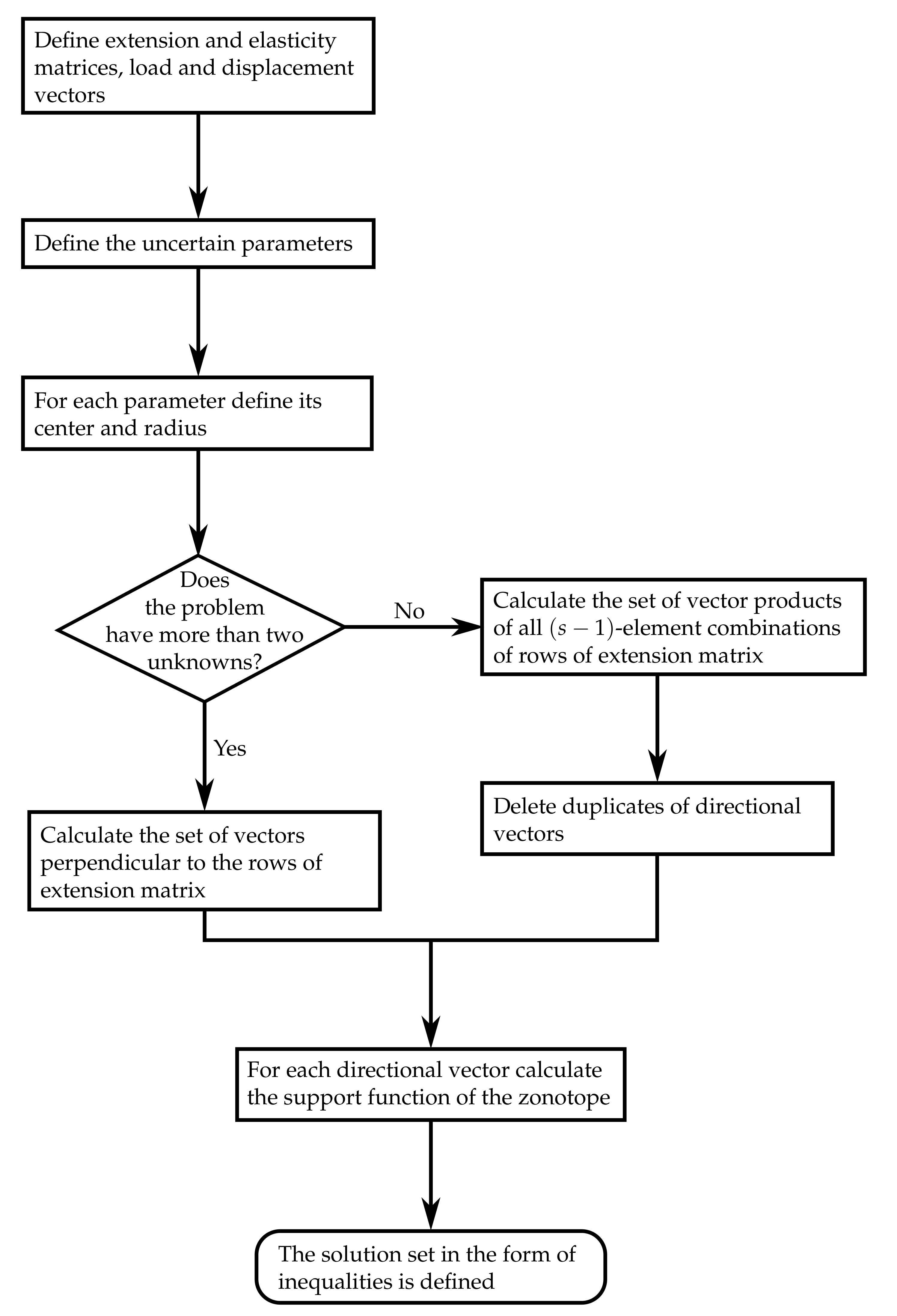
3. Description of the Solution Sets for Bar Structures

The algorithm presented in Section 2 is valid for structures that can be described by a system of algebraic equations. Adaptation of this algorithm to trusses and frames, separately, is shown below. In both cases, the equations derived in the works [18,19] are used. The equations describing the structure and the form of the zonotope $\mathcal{V}(\mathbf{q})$ are shown, assuming that the uncertain parameters are namely the stiffnesses of the bars and Young’s modulus, respectively for trusses and frames. In the present section one can find formulas which allow to determine solution sets ${\Xi }_{\mathrm{uni}}$.

3.1. Trusses

Let us take into the consideration a truss, which is composed of e bars and whose nodal deflections are described with s degrees of freedom. The linear system for trusses [18,19] is given by

$${\mathbf{B}}^{⊺}\mathbf{E}\mathbf{B}\mathbf{q}=\mathbf{Q},$$

(17)

where $\mathbf{E}=\mathrm{diag}(E_K)\in {\mathbb{R}}^{e\times e}$ ($K=1,\dots ,e$) is called elasticity matrix, $\mathbf{B}\in {\mathbb{R}}^{e\times s}$ extension matrix, $\mathbf{q}\in {\mathbb{R}}^s$ vector of unknown degrees of freedom and $\mathbf{Q}\in {\mathbb{R}}^s$ vector of node loads. Components $E_K=Y_K{A}_K/L_K$ contain the information about Young’s modulus $Y_K$, cross section $A_K$ and length $L_K$ of K-th bar. Components of matrix $\mathbf{B}$ are defined by the truss geometry and its construction method is described in [18,19].

Let the bars be characterized by uncertain stiffnesses $E_i$ and the imprecision $E_i$ be described by interval bounds, $E_i\in \left[E_i\right]$. The solution set (4) of system (17) can be written as

$${\Xi }_{\mathrm{uni}}=\left\{\mathbf{q}\in {\mathbb{R}}^s:\left(\exists \mathbf{E}\in \left[\mathbf{E}\right]\right)\left({\mathbf{B}}^{⊺}\mathbf{EB}\mathbf{q}=\mathbf{Q}\right)\right\},$$

(18)

where $\left[\mathbf{E}\right]=\mathrm{diag}(\left[E_1\right],\dots ,\left[E_e\right])$.

Let ${\mathbf{B}}^{(i)}$ be i-th row of matrix $\mathbf{B}$ (or i-th column of matrix ${\mathbf{B}}^{⊺}$). Then, due to the diagonality of matrix $\mathbf{E}$, it is possible to present the system (17) in the form

$$\sum _{i=1}^e\langle {\mathbf{B}}^{(i)},\mathbf{q}\rangle {\mathbf{B}}^{(i)}{E}_i=\mathbf{Q}.$$

(19)

The set $\mathcal{V}(\mathbf{q})$ (7) is given by formula

$$\mathcal{V}(\mathbf{q})=\mathbf{Q}+\sum _{i=1}^e\langle {\mathbf{B}}^{(i)},\mathbf{q}\rangle {\mathbf{B}}^{(i)}\ast \left[E_i\right].$$

(20)

It is worth to note that the scalar product $\langle {\mathbf{B}}^{(i)},\mathbf{q}\rangle$ defines the extension of i-th bar, while vectors ${\mathbf{B}}^{(i)}$ defines directions of zonotope $\mathcal{V}(\mathbf{q})$ edges. The set ${\mathcal{U}}^{+}$, necessary for finding the system of inequalities (16), is a set of vector products of all $(s-1)$-element combinations of vectors ${\mathbf{B}}^{(i)}$$(i=1,\dots ,e)$ or in case when $s=2$ is a set of all vectors perpendicular to ${\mathbf{B}}^{(i)}$. It is important that vectors obtained in this manner are independent from vector $\mathbf{q}$. Hence, the products (14) have the form

$$C^{(0)}(\mathbf{u})=\langle \mathbf{u},\mathbf{Q}\rangle ,C^{(i)}(\mathbf{u})=E_i\langle {\mathbf{B}}^{(i)},\mathbf{q}\rangle \langle {\mathbf{B}}^{(i)},\mathbf{u}\rangle .$$

(21)

For a more detailed illustration, the algorithm of searching for a solution set in the truss structure is shown in a flowchart in the Figure 1.

3.2. Frames

Let us take into the consideration a frame, which is composed of e bars and whose nodal deflections are described with s degrees of freedom. According to [18,19], the linear system for frames made of thin bars is given by

$$\left({\mathbf{B}}^{⊺}\mathbf{E}\mathbf{B}+2{({}^{\ast }\mathbf{B})}^{⊺}\mathbf{D}{}^{\ast }\mathbf{B}+{({}^{\ast }\mathbf{B})}^{⊺}\mathbf{D}{\mathbf{B}}^{\ast }+{({\mathbf{B}}^{\ast })}^{⊺}\mathbf{D}{}^{\ast }\mathbf{B}+2{({\mathbf{B}}^{\ast })}^{⊺}\mathbf{D}{\mathbf{B}}^{\ast }\right)\mathbf{q}=\mathbf{Q},$$

(22)

while for frames made of moderately thick bars by

$$\left({\mathbf{B}}^{⊺}\mathbf{E}\mathbf{B}+{({}^{\ast }\mathbf{B})}^{⊺}{\mathbf{D}}^{(1)}{}^{\ast }\mathbf{B}+{({}^{\ast }\mathbf{B})}^{⊺}{\mathbf{D}}^{(2)}{\mathbf{B}}^{\ast }+{({\mathbf{B}}^{\ast })}^{⊺}{\mathbf{D}}^{(2)}{}^{\ast }\mathbf{B}+{({\mathbf{B}}^{\ast })}^{⊺}{\mathbf{D}}^{(1)}{\mathbf{B}}^{\ast }\right)\mathbf{q}=\mathbf{Q},$$

(23)

in which $\mathbf{E}=\mathrm{diag}(E_K)\in {\mathbb{R}}^{e\times e}$, $\mathbf{D}=\mathrm{diag}(D_K)\in {\mathbb{R}}^{e\times e}$, ${\mathbf{D}}^{(1)}=\mathrm{diag}(D_K^{(1)})\in {\mathbb{R}}^{e\times e}$ and ${\mathbf{D}}^{(2)}=\mathrm{diag}(D_K^{(2)})\in {\mathbb{R}}^{e\times e}$ ($K=1,\dots ,e$) are constitutive matrices, $\mathbf{B}\in {\mathbb{R}}^{e\times s}$, ${}^{\ast }\mathbf{B}\in {\mathbb{R}}^{e\times s}$ and ${\mathbf{B}}^{\ast }\in {\mathbb{R}}^{e\times s}$ are geometrical matrices, $\mathbf{q}\in {\mathbb{R}}^s$ is a vector of unknown degrees of freedom and $\mathbf{Q}\in {\mathbb{R}}^s$ is a load vector. Identically like in trusses $E_K=Y_K{A}_K·L_K^{-1}$, while $D_K=2Y_K{I}_K·L_K^{-1}$, $D_K^{(1)}=2Y_K{I}_K{\mu }_K(1+3{\varrho }_K)·{(3L_K)}^{-1}$, $D_K^{(2)}=Y_K{I}_K{\mu }_K(1-6{\varrho }_K)·{(3L_K)}^{-1}$, in which ${\varrho }_K=Y_K{I}_K·{(H_K{L}_K^2)}^{-1}$, ${\mu }_K=6·{(12{\varrho }_K+1)}^{-1}$. Components of matrices $\mathbf{B}$, ${}^{\ast }\mathbf{B}$, ${\mathbf{B}}^{\ast }$ are defined by the frame geometry and its construction method is described in [18,19].

Let the bars be characterized by uncertain Young’s modulus $Y_K$, and the imprecision $Y_K$ be described by interval bounds $Y_K\in \left[Y_K\right]$, collected on the diagonal of parameter matrix $\left[\mathbf{p}\right]$.

It is then possible to decompose the matrices $\left[\mathbf{E}\right]$, $\left[\mathbf{D}\right]$, $\left[{\mathbf{D}}^{(1)}\right]$, $\left[{\mathbf{D}}^{(2)}\right]$ to the parts related and unrelated to the uncertain parameters, in form $\left[\mathbf{E}\right]=\left[\mathbf{p}\right]\widehat{\mathbf{E}}$, $\left[\mathbf{D}\right]=\left[\mathbf{p}\right]\widehat{\mathbf{D}}$, $\left[{\mathbf{D}}^{(1)}\right]=\left[\mathbf{p}\right]{\widehat{\mathbf{D}}}^{(1)}$ and $\left[{\mathbf{D}}^{(2)}\right]=\left[\mathbf{p}\right]{\widehat{\mathbf{D}}}^{(2)}$, where

$$\begin{array}{cc}\hfill & \widehat{\mathbf{E}}=\mathrm{diag}\left(\frac{A_K}{L_K}\right),\widehat{\mathbf{D}}=\mathrm{diag}(2I_K/L_K),\hfill \\ \hfill & {\widehat{\mathbf{D}}}^{(1)}=\mathrm{diag}\left(\frac{2I_K{\mu }_K(1+3{\varrho }_K)}{3L_K}\right),{\widehat{\mathbf{D}}}^{(2)}=\mathrm{diag}\left(\frac{I_K{\mu }_K(1-6{\varrho }_K)}{3L_K}\right)\hfill \end{array}$$

(24)

and $\left[\mathbf{p}\right]=\mathrm{diag}(\left[p_i\right])$ ($i=1,2,...,e$). Then the solution set (4) of the system (22) can be written as

$$\begin{array}{cc}\hfill & {\Xi }_{\mathrm{uni}}=\left\{\mathbf{q}\in {\mathbb{R}}^s:\exists \mathbf{p}\in \left[\mathbf{p}\right],\left({\mathbf{B}}^{⊺}\left(\mathbf{p}\widehat{\mathbf{E}}\right)\mathbf{B}+2{({}^{\ast }\mathbf{B})}^{⊺}\left(\mathbf{p}\widehat{\mathbf{D}}\right){}^{\ast }\mathbf{B}+\right.\right.\hfill \\ \hfill & \left.\left.+{({}^{\ast }\mathbf{B})}^{⊺}\left(\mathbf{p}\widehat{\mathbf{D}}\right){\mathbf{B}}^{\ast }+{({\mathbf{B}}^{\ast })}^{⊺}\left(\mathbf{p}\widehat{\mathbf{D}}\right){}^{\ast }\mathbf{B}+2{({\mathbf{B}}^{\ast })}^{⊺}\left(\mathbf{p}\widehat{\mathbf{D}}\right){\mathbf{B}}^{\ast }\right)\mathbf{q}=\mathbf{Q}\right\},\hfill \end{array}$$

(25)

while for the system (23) as

$$\begin{array}{cc}\hfill & {\Xi }_{\mathrm{uni}}=\left\{\mathbf{q}\in {\mathbb{R}}^s:\exists \mathbf{p}\in \left[\mathbf{p}\right],\left({\mathbf{B}}^{⊺}\left(\mathbf{p}\widehat{\mathbf{E}}\right)\mathbf{B}+{({}^{\ast }\mathbf{B})}^{⊺}\left(\mathbf{p}{\widehat{\mathbf{D}}}^{(1)}\right){}^{\ast }\mathbf{B}+\right.\right.\hfill \\ \hfill & \left.\left.+{({}^{\ast }\mathbf{B})}^{⊺}\left(\mathbf{p}{\widehat{\mathbf{D}}}^{(2)}\right){\mathbf{B}}^{\ast }+{({\mathbf{B}}^{\ast })}^{⊺}\left(\mathbf{p}{\widehat{\mathbf{D}}}^{(2)}\right){}^{\ast }\mathbf{B}+{({\mathbf{B}}^{\ast })}^{⊺}\left(\mathbf{p}{\widehat{\mathbf{D}}}^{(1)}\right){\mathbf{B}}^{\ast }\right)\mathbf{q}=\mathbf{Q}\right\}.\hfill \end{array}$$

(26)

Let ${\mathbf{B}}^{(i)}$, ${({}^{\ast }\mathbf{B})}^{(i)}$, ${({\mathbf{B}}^{\ast })}^{(i)}$ be relatively the i-th rows of matrices $\mathbf{B}$, ${}^{\ast }\mathbf{B}$, ${\mathbf{B}}^{\ast }$ (or i-th columns of matrices ${\mathbf{B}}^{⊺}$, ${({}^{\ast }\mathbf{B})}^{⊺}$, ${({\mathbf{B}}^{\ast })}^{⊺}$). Then, due to the diagonality of matrices $\mathbf{E}$, $\mathbf{D}$, ${\mathbf{D}}^{(1)}$, ${\mathbf{D}}^{(2)}$, it is possible to present the systems (22) and (23) relatively in the form

$$\begin{array}{cc}\hfill & \sum _{i=1}^e\left({\widehat{E}}_{ii}\langle {\mathbf{B}}^{(i)},\mathbf{q}\rangle {\mathbf{B}}^{(i)}+{\widehat{D}}_{ii}\langle {({}^{\ast }\mathbf{B})}^{(i)},\mathbf{q}\rangle \left(2{({}^{\ast }\mathbf{B})}^{(i)}+{({\mathbf{B}}^{\ast })}^{(i)}\right)+\right.\hfill \\ \hfill & \left.+{\widehat{D}}_{ii}\langle {({\mathbf{B}}^{\ast })}^{(i)},\mathbf{q}\rangle \left(2{({\mathbf{B}}^{\ast })}^{(i)}+{({}^{\ast }\mathbf{B})}^{(i)}\right)\right)p_i=\mathbf{Q}\hfill \end{array}$$

(27)

and

$$\begin{array}{cc}\hfill & \sum _{i=1}^e\left({\widehat{E}}_{ii}\langle {\mathbf{B}}^{(i)},\mathbf{q}\rangle {\mathbf{B}}^{(i)}+{\widehat{D}}_{ii}^{(1)}\left(\langle {({}^{\ast }\mathbf{B})}^{(i)},\mathbf{q}\rangle {({}^{\ast }\mathbf{B})}^{(i)}+\langle {({\mathbf{B}}^{\ast })}^{(i)},\mathbf{q}\rangle {({\mathbf{B}}^{\ast })}^{(i)}\right)+\right.\hfill \\ \hfill & \left.+{\widehat{D}}_{ii}^{(2)}\left(\langle {({}^{\ast }\mathbf{B})}^{(i)},\mathbf{q}\rangle {({\mathbf{B}}^{\ast })}^{(i)}+\langle {({\mathbf{B}}^{\ast })}^{(i)},\mathbf{q}\rangle {({}^{\ast }\mathbf{B})}^{(i)}\right)\right)p_i=\mathbf{Q},\hfill \end{array}$$

(28)

where $p_i\in \left[p_i\right]$ are imprecise. It means that the set $\mathcal{V}(\mathbf{q})$ has the form

$$\begin{array}{cc}\hfill & \mathcal{V}(\mathbf{q})=-\sum _{i=1}^e\left({\widehat{E}}_{ii}\langle {\mathbf{B}}^{(i)},\mathbf{q}\rangle {\mathbf{B}}^{(i)}+{\widehat{D}}_{ii}\langle {({}^{\ast }\mathbf{B})}^{(i)},\mathbf{q}\rangle \left(2{({}^{\ast }\mathbf{B})}^{(i)}+{({\mathbf{B}}^{\ast })}^{(i)}\right)+\right.\hfill \\ \hfill & \left.+{\widehat{D}}_{ii}\langle {({\mathbf{B}}^{\ast })}^{(i)},\mathbf{q}\rangle \left(2{({\mathbf{B}}^{\ast })}^{(i)}+{({}^{\ast }\mathbf{B})}^{(i)}\right)\right)\ast \left[p_i\right]+\mathbf{Q}\hfill \end{array}$$

(29)

for the frame made of thin bars and

$$\begin{array}{cc}\hfill & \mathcal{V}(\mathbf{q})=\mathbf{Q}-\sum _{i=1}^e\left({\widehat{E}}_{ii}\langle {\mathbf{B}}^{(i)},\mathbf{q}\rangle {\mathbf{B}}^{(i)}+{\widehat{D}}_{ii}^{(1)}\left(\langle {({}^{\ast }\mathbf{B})}^{(i)},\mathbf{q}\rangle {({}^{\ast }\mathbf{B})}^{(i)}+\langle {({\mathbf{B}}^{\ast })}^{(i)},\mathbf{q}\rangle {({\mathbf{B}}^{\ast })}^{(i)}\right)+\right.\hfill \\ \hfill & \left.+{\widehat{D}}_{ii}^{(2)}\left(\langle {({}^{\ast }\mathbf{B})}^{(i)},\mathbf{q}\rangle {({\mathbf{B}}^{\ast })}^{(i)}+\langle {({\mathbf{B}}^{\ast })}^{(i)},\mathbf{q}\rangle {({}^{\ast }\mathbf{B})}^{(i)}\right)\right)\ast \left[p_i\right]\hfill \end{array}$$

(30)

for the frame made of moderately thick bars.

Obtaining the description of the solution set in the form of inequalities is possible with the use of (16). For thin bars the scalar products (14) are in the form

$$\begin{array}{cc}\hfill & C^{(i)}(\mathbf{u})={\widehat{E}}_{ii}\langle {\mathbf{B}}^{(i)},\mathbf{q}\rangle \langle {\mathbf{B}}^{(i)},\mathbf{u}\rangle +{\widehat{D}}_{ii}\langle {({}^{\ast }\mathbf{B})}^{(i)},\mathbf{q}\rangle \langle 2{({}^{\ast }\mathbf{B})}^{(i)}+{({\mathbf{B}}^{\ast })}^{(i)},\mathbf{u}\rangle +\hfill \\ \hfill & +{\widehat{D}}_{ii}\langle {({\mathbf{B}}^{\ast })}^{(i)},\mathbf{q}\rangle \langle 2{({\mathbf{B}}^{\ast })}^{(i)}+{({}^{\ast }\mathbf{B})}^{(i)},\mathbf{u}\rangle ,\hfill \end{array}$$

(31)

while for the moderately thick bars

$$\begin{array}{cc}\hfill & C^{(i)}(\mathbf{u})={\widehat{E}}_{ii}\langle {\mathbf{B}}^{(i)},\mathbf{q}\rangle \langle {\mathbf{B}}^{(i)},\mathbf{u}\rangle +{\widehat{D}}_{ii}^{(1)}\langle {({}^{\ast }\mathbf{B})}^{(i)},\mathbf{q}\rangle \langle {({}^{\ast }\mathbf{B})}^{(i)},\mathbf{u}\rangle +\hfill \\ \hfill & +{\widehat{D}}_{ii}^{(1)}\langle {({\mathbf{B}}^{\ast })}^{(i)},\mathbf{q}\rangle \langle {({\mathbf{B}}^{\ast })}^{(i)},\mathbf{u}\rangle +{\widehat{D}}_{ii}^{(2)}\langle {({}^{\ast }\mathbf{B})}^{(i)},\mathbf{q}\rangle \langle {({\mathbf{B}}^{\ast })}^{(i)},\mathbf{u}\rangle +\hfill \\ \hfill & +{\widehat{D}}_{ii}^{(2)}\langle {({\mathbf{B}}^{\ast })}^{(i)},\mathbf{q}\rangle \langle {({}^{\ast }\mathbf{B})}^{(i)},\mathbf{u}\rangle ,i=1,2,3\hfill \end{array}$$

(32)

and for both cases

$$C^{(0)}(\mathbf{u})=\langle \mathbf{Q},\mathbf{u}\rangle .$$

(33)

From the form of zonotope (29) steams that the set ${\mathcal{U}}^{+}$ for thin bars should be determined as a set of vector products of all $(s-1)$-element combinations of vectors

$$\begin{array}{cc}\hfill & \left({\widehat{E}}_{ii}\langle {\mathbf{B}}^{(i)},\mathbf{q}\rangle {\mathbf{B}}^{(i)}+{\widehat{D}}_{ii}\langle {({}^{\ast }\mathbf{B})}^{(i)},\mathbf{q}\rangle \left(2{({}^{\ast }\mathbf{B})}^{(i)}+{({\mathbf{B}}^{\ast })}^{(i)}\right)+{\widehat{D}}_{ii}\langle {({\mathbf{B}}^{\ast })}^{(i)},\mathbf{q}\rangle \left(2{({\mathbf{B}}^{\ast })}^{(i)}+{({}^{\ast }\mathbf{B})}^{(i)}\right)\right)\hfill \end{array}$$

(34)

$(i=1,\dots ,e)$. In the case of the structure made of moderately thick bars the set ${\mathcal{U}}^{+}$ should be determined by analogy, but with the use of vectors from (30). It should be noted that vectors obtained in this manner can be dependent on the vector $\mathbf{q}$.

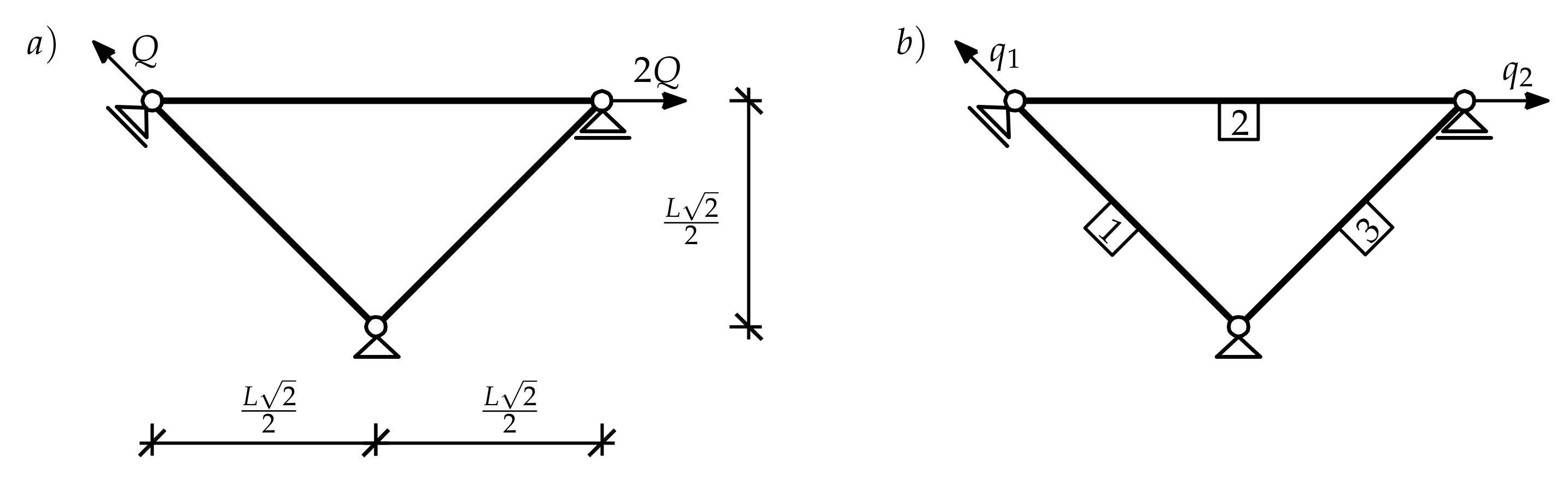
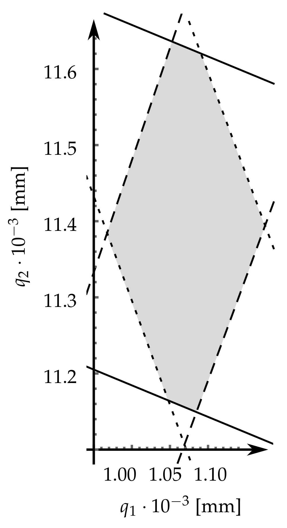
4. Illustrative Example

The example illustrating the proposed algorithm for obtaining a solution set is presented below. As an example, a truss structure is selected for which the system of equations is relatively simple. The essence of the example is to explain the construction of the system of inequalities, which describes the solution set and to show the advantages of the formulation, being aware of its disadvantages.

Let us consider a truss composed of three bars, whose geometry and load is presented in Figure 2. The truss consists of three bars and three nodes. It is loaded with two concentrated forces. The extension matrix $\mathbf{B}$, load vector $\mathbf{Q}$ and vector of nodal displacements $\mathbf{q}$ are given by

$$\mathbf{B}=\left(\begin{array}{cc}1& 0\\ \frac{\sqrt{2}}{2}& 1\\ 0& \frac{\sqrt{2}}{2}\end{array}\right),\mathbf{Q}=\left(\begin{array}{c}Q\\ 2Q\end{array}\right),\mathbf{q}=\left(\begin{array}{c}{q}_1\\ q_2\end{array}\right).$$

(35)

Let the bars be characterized by uncertain Young’s moduli. Then, it is possible to decompose elasticity matrix $\mathbf{E}$ into parts connected and not connected with uncertain parameters, in the form

$$\left[\mathbf{E}\right]=\left[\mathbf{p}\right]\widehat{\mathbf{E}}=\left(\begin{array}{ccc}\left[p_1\right]& 0& 0\\ 0& \left[p_2\right]& 0\\ 0& 0& \left[p_3\right]\end{array}\right)\left(\begin{array}{ccc}\frac{A_1}{L}& 0& 0\\ 0& \frac{A_2}{\sqrt{2}L}& 0\\ 0& 0& \frac{A_3}{L}\end{array}\right),$$

(36)

with uncertain values of bars elasticity $\left[E_1\right]=\left[p_1\right]A_1/L$, $\left[E_2\right]=\left[p_2\right]A_2/(\sqrt{2}L)$, $\left[E_3\right]=\left[p_3\right]A_3/L$.

Let us consider the system of inequalities (15). The set $\mathcal{V}(\mathbf{q})$, defined by (7), is given by

$$\begin{array}{cc}\hfill & \mathcal{V}(\mathbf{q})=\left(\begin{array}{c}Q\\ 2Q\end{array}\right)-q_1\left(\begin{array}{c}1\\ 0\end{array}\right)\ast \left[E_1\right]-\left(\frac{1}{\sqrt{2}}{q}_1+q_2\right)\left(\begin{array}{c}\frac{1}{\sqrt{2}}\\ 1\end{array}\right)\ast \left[E_2\right]-\frac{1}{\sqrt{2}}{q}_2\left(\begin{array}{c}0\\ 1\end{array}\right)\ast \left[E_3\right].\hfill \end{array}$$

(37)

It is worth to note that the decomposition of (37) contains vectors ${\mathbf{B}}^{(i)}$

$${\mathbf{B}}^{(1)}=\left(\begin{array}{c}1\\ 0\end{array}\right),{\mathbf{B}}^{(2)}=\left(\begin{array}{c}\frac{1}{\sqrt{2}}\\ 1\end{array}\right),{\mathbf{B}}^{(3)}=\left(\begin{array}{c}0\\ \frac{1}{\sqrt{2}}\end{array}\right),$$

(38)

which are the rows of matrix $\mathbf{B}$.

Let us define vectors ${\mathbf{u}}^{(i)}$ ($i=1,2,3$) perpendicular to ${\mathbf{B}}^{(i)}$ and in the same time perpendicular to zonotope $\mathcal{V}(\mathbf{q})$ edges

$${\mathbf{u}}^{(1)}=\left(\begin{array}{c}0\\ 1\end{array}\right),{\mathbf{u}}^{(2)}=\left(\begin{array}{c}1\\ -\frac{1}{\sqrt{2}}\end{array}\right),{\mathbf{u}}^{(3)}=\left(\begin{array}{c}1\\ 0\end{array}\right).$$

(39)

Then the system of inequalities (16) is given by

$$\begin{array}{cc}\hfill & {\mathbf{u}}^{(1)}\Rightarrow |2Q-\left(\frac{1}{\sqrt{2}}{q}_1+q_2\right)E_2^{\mathrm{c}}-\frac{1}{\sqrt{2}}{q}_2{E}_3^{\mathrm{c}}|\le |\frac{1}{\sqrt{2}}{q}_1+q_2|E_2^{\Delta }+\frac{1}{\sqrt{2}}\left|q_2\right|E_3^{\mathrm{c}},\hfill \\ \hfill & {\mathbf{u}}^{(2)}\Rightarrow |Q-\frac{2}{\sqrt{2}}Q-q_1{E}_1^{\mathrm{c}}-\frac{1}{2\sqrt{2}}{q}_2{E}_3^{\mathrm{c}}|\le |q_1|E_1^{\Delta }+\frac{1}{2\sqrt{2}}\left|q_2\right|E_3^{\mathrm{c}},\hfill \\ \hfill & {\mathbf{u}}^{(3)}\Rightarrow |Q-q_1{E}_1^{\mathrm{c}}-\left(\frac{1}{2}{q}_1+\frac{1}{\sqrt{2}}{q}_2\right)E_2^{\mathrm{c}}|\le |q_1|E_1^{\Delta }+\left|\frac{1}{2}{q}_1+\frac{1}{\sqrt{2}}{q}_2\right|E_2^{\Delta }.\hfill \end{array}$$

(40)

When bars are characterized with cross-section area $A_i=6.67 {\mathrm{cm}}^2$ ($i=1,2,3$) and the load is $Q=1 \mathrm{kN}$, the intervals of uncertainty equal $\left[E_2\right]\cong \left[990-20,990+20\right]\mathrm{kN}/\mathrm{cm}$ and $\left[E_i\right]\cong \left[1400-28,1400+28\right]\mathrm{kN}/\mathrm{cm}$ ($i=1,3$), the system (40) can be presented in the form

$$\begin{array}{cc}\hfill & {\mathbf{u}}^{(1)}\Rightarrow |2-700.24q_1-1690.53q_2|\le 14.00|q_2|+19.81|0.71q_1+q_2|,\hfill \\ \hfill & {\mathbf{u}}^{(2)}\Rightarrow |-0.41-1400.48q_1+495.15q_2|\le 28.01|q_1|+9.90|q_2|,\hfill \\ \hfill & {\mathbf{u}}^{(3)}\Rightarrow |1-1895.63q_1-700.24q_2|\le 28.01|q_1|+19.81|0.5q_1+0.71q_2|,\hfill \end{array}$$

(41)

where $q_1$, $q_2$ are in $\mathrm{cm}$.

The above presented system of inequalities describes the set ${\Xi }_{\mathrm{uni}}$. Its graphical interpretation is presented in Figure 3. Solid lines indicate the region of acceptable solutions defined by inequality obtained for ${\mathbf{u}}^{(1)}$, dashed for ${\mathbf{u}}^{(2)}$ and dotted for ${\mathbf{u}}^{(3)}$. One should note that the set is limited by straight lines, not curves.

The significant property of the stiffness matrix can be observed after decomposing it into the sum of three matrices assigned to subsequent uncertain parameters

$$\left[\mathbf{K}\right]=\sum _{i=1}^3\left[E_i\right]{\mathbf{K}}^{(i)},{\mathbf{K}}^{(1)}=\left(\begin{array}{cc}1& 0\\ 0& 0\end{array}\right),{\mathbf{K}}^{(2)}=\left(\begin{array}{cc}\frac{1}{2}& \frac{1}{\sqrt{2}}\\ \frac{1}{\sqrt{2}}& 1\end{array}\right),{\mathbf{K}}^{(3)}=\left(\begin{array}{cc}0& 0\\ 0& \frac{1}{2}\end{array}\right).$$

(42)

Each of three matrices ${\mathbf{K}}^{(i)}$ ($i=1,2,3$) has rank 1. It means that the boundary of set ${\Xi }_{\mathrm{uni}}$ is composed of line segments, which is justified by the above considerations.

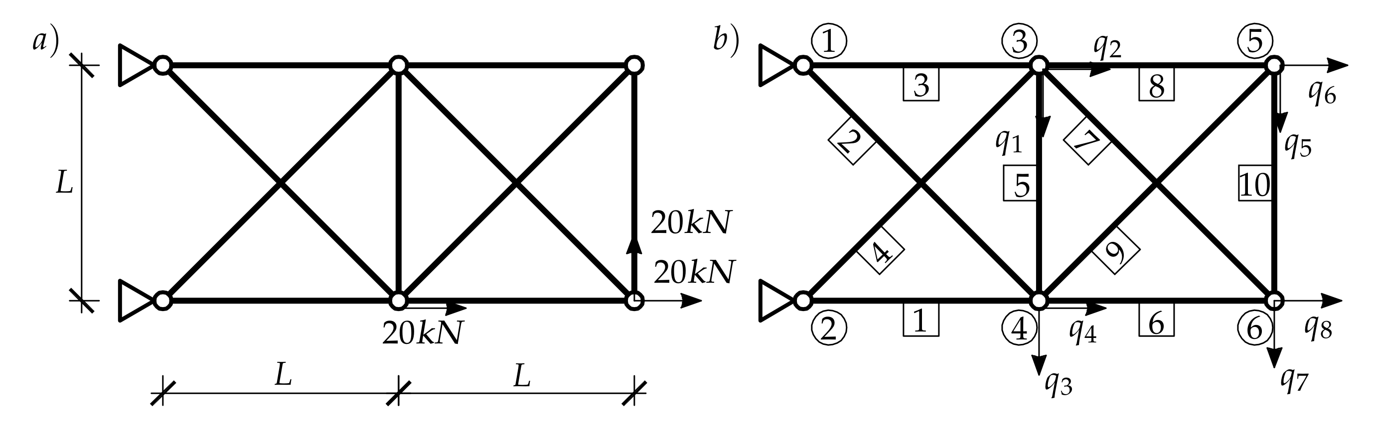
5. Numerical Example

The truss shown in the Section 4 was characterized by a small number of bars and unknowns. The set of solutions for a structure with a greater number of unknowns and bars, which causes an increase of the dimensions of the matrix $\mathbf{B}$, lies in a multidimensional space. The application of the present algorithm to such a structure leads to obtaining much more complex sets of inequalities.

Let us consider a truss shown in Figure 4. The truss is composed of ten bars, which are characterized by uncertain cross-section area with nominal value of $1{\mathrm{cm}}^2$. The Young’s modulus, force P and length L are assumed to be $100\mathrm{GPa}$, $20\mathrm{kN}$ and $500\mathrm{cm}$, respectively.

The extension matrix, elasticity matrix and load vector are given as follows

$$\mathbf{B}=\left(\begin{array}{cccccccc}0& 0& 0& 1& 0& 0& 0& 0\\ 0& 0& \frac{1}{\sqrt{2}}& \frac{1}{\sqrt{2}}& 0& 0& 0& 0\\ 0& 1& 0& 0& 0& 0& 0& 0\\ -\frac{1}{\sqrt{2}}& \frac{1}{\sqrt{2}}& 0& 0& 0& 0& 0& 0\\ -1& 0& 1& 0& 0& 0& 0& 0\\ 0& 0& 0& -1& 0& 0& 0& 1\\ -\frac{1}{\sqrt{2}}& -\frac{1}{\sqrt{2}}& 0& 0& 0& 0& \frac{1}{\sqrt{2}}& \frac{1}{\sqrt{2}}\\ 0& -1& 0& 0& 0& 1& 0& 0\\ 0& 0& \frac{1}{\sqrt{2}}& -\frac{1}{\sqrt{2}}& -\frac{1}{\sqrt{2}}& \frac{1}{\sqrt{2}}& 0& 0\\ 0& 0& 0& 0& -1& 0& 1& 0\end{array}\right),$$

(43)

$$\begin{array}{cc}\hfill & \left[\mathbf{E}\right]=\left[\mathbf{p}\right]\widehat{\mathbf{E}},\left[\mathbf{p}\right]=\mathrm{diag}\left(\left[p_1\right],\left[p_2\right],\dots ,\left[p_{10}\right]\right),\hfill \\ \hfill & \widehat{\mathbf{E}}=\frac{Y}{L}\mathrm{diag}\left(1,0,\frac{1}{\sqrt{2}},1,\frac{1}{\sqrt{2}},1,1,\frac{1}{\sqrt{2}},1,\frac{1}{\sqrt{2}},1\right),\hfill \end{array}$$

(44)

$$Q={\left(0,0,0,P,0,0,-P,P\right)}^{⊺}\mathrm{kN}.$$

(45)

The maximum number of inequalities necessary for definition of the solution set ${\Xi }_{\mathrm{uni}}$ equals $\left(\genfrac{}{}{0pt}{}{e}{s-1}\right)=\left(\genfrac{}{}{0pt}{}{10}{7}\right)=120$ and the set $\mathcal{U}$ consists of vector products of all $(s-1)$-element combinations of vectors ${\mathbf{B}}^{(i)}$$(i=1,2,\cdots ,e)$, which, after deletion of duplicates, is 42. The set of vectors, basing on which it is possible to build the inequalities defined by (16), is presented in Appendix B.

The proposed truss is analysed in [22], where authors obtain an exact bound of horizontal displacement of node 6 with the use of sensitivity bound techniques. Due to the convexity of the solution set ${\Xi }_{\mathrm{uni}}$ the maximum possible value of the analysed displacement is defined by vertices or edges of polytope ${\Xi }_{\mathrm{uni}}$. It should be mentioned that the analysis of all possible cases of uncertain parameters bounds leads to the set of solution points, not all of which are the vertices of the solution polytope [23]. The set of inequalities (16), which defines the exact solution set ${\Xi }_{\mathrm{uni}}$, allows the verification of the obtained result.

It should be noted that the proposed technique can be applied not only to trusses, but also to other structures that can be described by a system of algebraic equations. It is not rational to try to solve larger problems directly with the proposed algorithm. Such an implementation is possible, but there is a need to develop a different procedure. This, however, should be the subject of further research beyond this article. Proposals for applying the method in its current form are presented in the next section.

6. Practical Implications

The tasks presented in Section 4 and Section 5 show the significant advantages of the proposed formulation. The considerations, from the formulation to the result obtained, are accurate within the theory and do not contain approximations. The obtained results give information about the shape of the solution set. The knowledge that the set is limited by the straight lines or planes makes it possible to select an appropriate technique when analysing larger tasks. When the faces of a set are described by planes, it is possible to use linear programming to define the set numerically.

Interval methods, often used in uncertainty analysis, lead to box set estimates. The graphically presented set, in the case of 2D, is then limited by straight lines parallel to the axis of the coordinate system, and in multidimensional cases by the corresponding planes. Within this approach, the resulting set is at best the smallest possible box containing the exact solution set. The knowledge of the exact shape of the set obtained by the present method allows to determine the degree of overestimation of the result. This can be done, for example, by comparing the volumes of individual sets.

Although the proposed method has the limitations connected with the size of the problem it allows one to obtain the exact solution given in the form of set of inequalities. The possibility of determination of exact solution set allows one to prepare benchmark solutions that can be used to determine the accuracy of other methods. Only the small problems are shown in the paper, because their solution sets can be presented and analysed graphically. The level of complexity of the solution increases for large problems. Therefore, it is necessary to search for effective algorithms and ways to selectively assess the results of calculations. That is not included in the present paper.

Knowing the exact solution set allows one to calibrate other computational methods and algorithms. This may allow to increase their accuracy, and thus minimise the impact of uncertain parameters on the calculation results. It is important because uncertain parameters occur at many stages of structure design. Reducing their impact can improve the design process and make it easier to create more reliable structures.

7. Conclusions

In the present paper the method of constructing the solution set of an engineering structure, based on the convex sets analysis methods is presented. The proposed method, opposed to algorithms providing estimations, allows one to obtain the exact solution set in the form of polyhedron called zonotope, described with Minkowski sum of finite set of points and line segments. The description is given in the form of system of inequalities. It is a novel approach as far as applications to engineering structures are concerned.

The presented method can be applied if the structure is described by a system of linear algebraic equations and relates to structures with independent uncertain parameters. Presenting the matrix of the system of equations as the sum of matrices dependent on separated uncertain parameters allows one to conclude about the impact of individual uncertain parameters on the shape and size of the solution set and to assess the impact of individual parameters on the behaviour of the entire structure. Furthermore, the matrices of decomposition make it possible to determine whether the edges of the solution set are described by hyperplanes or non-flat hypersurfaces. Moreover, because the formulation is devoid of approximations it is not sensitive for perturbed data.

Due to generality and accuracy, the present approach has its limitations. The method provides solution sets for structures described by the stiffness matrix of particular form. However, this does not imply the limitation to trusses. The method applies to any structure made of thin and thick bars. Because the level of complexity of the solution increases for large tasks, it is necessary to search for effective algorithms and ways to selectively assess the results of calculations, which is not included in the present paper.

What is important, the proposed description takes into account not only the bounds of individual unknowns, but also allows for the relation between them. It is worth noting that the calculations carried out using the algorithms used in the present paper are valid for any level of uncertainty. The presented considerations relate to the uncertainty of Young’s modulus, but remain valid for the uncertainty of geometrical parameters of bars’ structures. Such solutions in the field of general bar theory are not known in the literature. Few attempts at solutions and estimates relate to trusses.

Furthermore, the proposed description of solution sets makes it possible to analyse the properties of these sets. With the use of the linear programming methods, it is possible to obtain the smallest boxes containing the described sets, which will allow the comparison of given sets with the results published in the literature. As the quantitative parameter for comparison one can use for example the volume of received solution sets.

References

1. Pełczyński, J. On Mathematical Descriptions of Uncertain Parameters in Engineering Structures. Arch. Civ. Eng. 2018, 64, 2–19. [Google Scholar] [CrossRef] [Green Version]
2. Moens, D.; Vandepitte, D. A survey of non-probabilistic uncertainty treatment in finite element analysis. Comput. Methods Appl. Mech. Eng. 2005, 194, 1527–1555. [Google Scholar] [CrossRef]
3. Radoń, U. Reliability analysis of Mises truss. Arch. Civ. Mech. Eng. 2011, 11, 723–738. [Google Scholar] [CrossRef]
4. Stefanou, G. The stochastic finite element method: Past, present and future. Comput. Methods Appl. Mech. Eng. 2009, 198, 1031–1051. [Google Scholar] [CrossRef] [Green Version]
5. Korkmaz, K.A.; Demir, F.; Tekeli, H. Uncertainty modelling of critical column buckling for reinforced concrete buildings. Sadhana 2011, 36, 267. [Google Scholar] [CrossRef]
6. Guo, S.X.; Lu, Z.Z. A non-probabilistic robust reliability method for analysis and design optimization of structures with uncertain-but-bounded parameters. Appl. Math. Model. 2015, 39, 1985–2002. [Google Scholar] [CrossRef]
7. Smith, A.P.; Garloff, J.; Werkle, H. Verified solution for a simple truss structure with uncertain node locations. In Proceedings of the 18th International Conference on the Application of Computer Science and Mathematics in Architecture and Civil Engineering, Weimar, Germany, 7–9 July 2009. [Google Scholar]
8. Wang, L.; Xiong, C.; Wang, X.; Xu, M.; Li, Y. A dimension-wise method and its improvement for multidisciplinary interval uncertainty analysis. Appl. Math. Model. 2018, 59, 680–695. [Google Scholar] [CrossRef]
9. Xiong, C.; Wang, L.; Liu, G.; Shi, Q. An iterative dimension-by-dimension method for structural interval response prediction with multidimensional uncertain variables. Aerosp. Sci. Technol. 2019, 86, 572–581. [Google Scholar] [CrossRef]
10. Wang, L.; Liu, Y.; Liu, Y. An inverse method for distributed dynamic load identification of structures with interval uncertainties. Adv. Eng. Softw. 2019, 131, 77–89. [Google Scholar] [CrossRef]
11. Niczyj, J. Multi-Criterion Reliability Optimization and Technical Assessment of Bar Structures on the Background of Fuzzy Set Theory; Szczecin Univ. of Technology Publishers: Szczecin, Poland, 2003. (In Polish) [Google Scholar]
12. De Mulder, W.; Moens, D.; Vandepitte, D. Modeling uncertainty in the context of finite element models with distance-based interpolation. In Proceedings of the 1st International Symposium on Uncertainty Quantification and Stochastic Modeling, Maresias, Brazil, 16 February–2 March 2012. [Google Scholar]
13. Harirchian, E.; Lahmer, T. Improved Rapid Visual Earthquake Hazard Safety Evaluation of Existing Buildings Using a Type-2 Fuzzy Logic Model. Appl. Sci. 2020, 10, 2375. [Google Scholar] [CrossRef] [Green Version]
14. Fink, T. BIM for Structural Engineering. In Building Information Modeling; Springer: Berlin, Germany, 2018; pp. 329–336. [Google Scholar]
15. Alizadehsalehi, S.; Hadavi, A.; Huang, J.C. From BIM to extended reality in AEC industry. Autom. Constr. 2020, 116, 103254. [Google Scholar] [CrossRef]
16. Muhanna, R.L.; Mullen, R.L.; Zhang, H. Interval finite element as a basis for generalized models of uncertainty in engineering mechanics. Reliab. Comput. 2007, 13, 173–194. [Google Scholar] [CrossRef]
17. Shary, S.P. On optimal solution of interval linear equations. SIAM J. Numer. Anal. 1995, 32, 610–630. [Google Scholar] [CrossRef]
18. Lewiński, T. On algebraic equations of elastic trusses, frames and grillages. J. Theor. Appl. Mech. 2001, 39, 307–322. [Google Scholar]
19. Pełczyński, J.; Gilewski, W. Algebraic Formulation for Moderately Thick Elastic Frames, Beams, Trusses, and Grillages within Timoshenko Theory. Math. Probl. Eng. 2019, 2019, 7545473. [Google Scholar] [CrossRef]
20. Dessombz, O.; Thouverez, F.; Laîné, J.P.; Jézéquel, L. Analysis of mechanical systems using interval computations applied to finite element methods. J. Sound Vib. 2001, 239, 949–968. [Google Scholar] [CrossRef] [Green Version]
21. Neumaier, A.; Pownuk, A. Linear systems with large uncertainties, with applications to truss structures. Reliab. Comput. 2007, 13, 149–172. [Google Scholar] [CrossRef]
22. Du, J.; Du, Z.; Wei, Y.; Zhang, W.; Guo, X. Exact response bound analysis of truss structures via linear mixed 0-1 programming and sensitivity bounding technique. Int. J. Numer. Methods Eng. 2018, 116, 21–42. [Google Scholar] [CrossRef]
23. Gilewski, W.; Pełczyński, J.; Rzeżuchowski, T.; Wąsowski, J. Truss structures with uncertain parameters–geometrical interpretation of the solution based on properties of convex sets. In Theoretical Foundations of Civil Engineering Vol. 7: Structural Mechanics; Jemioło, S., Gajewski, M., Eds.; Warsaw University of Technology Publisher House: Warszawa, Poland, 2016; pp. 41–52. [Google Scholar]
24. Pełczyński, J.; Rzeżuchowski, T.; Wąsowski, J. Description of united solution sets by inequalities for truss structures. In Proceedings of the 4th ECCOMAS Young Investigators Conference (YIC 2017), Milan, Italy, 13–15 September 2017. [Google Scholar]
25. Rzeżuchowski, T.; Wąsowski, J. Characterization of AE solution sets of parametric linear systems based on the techniques of convex sets. Linear Algebra Appl. 2017, 533, 468–490. [Google Scholar] [CrossRef]
Figure 1. Diagram of searching for a solution set in the form of inequalities, assuming truss structure.
Applsci 10 06864 g001
Figure 2. Truss geometry and supports with (a) loads and (b) degrees of freedom.
Applsci 10 06864 g002
Figure 3. Solution set Ξ uni .
Applsci 10 06864 g003
Figure 4. Truss geometry and supports with (a) loads and (b) degrees of freedom.
Applsci 10 06864 g004