Kalman Filter-Based Adaptive Delay Compensation for Benchmark Problem in Real-Time Hybrid Simulation

Abstract

Real-time hybrid simulation (RTHS) is a versatile, effective, and promising experimental method used to evaluate the structural performance under dynamic loads. In RTHS, the emulated structure is divided into a numerically simulated substructure (NS) and a physically tested substructure (PS), and a transfer system is used to ensure the force equilibrium and deformation compatibility between the substructures. Owing to the inherent dynamics of the PS and transfer system (referred to as a control plant in this study), there is a time-delay between the displacement command and measurement. This causes de-synchronization between the boundary of the PS and NS, and affects the stability and accuracy of the RTHS. In this study, a Kalman filter-based adaptive delay compensation (KF-ADC) method is proposed to address this issue. In this novel method, the control plant is represented by a discrete-time model, whose coefficients are time-varying and are estimated online by the KF using the displacement commands and measurements. Based on this time-varying model, the delay compensator is constructed employing the desired displacements. The KF performance is investigated theoretically and numerically. To assess the performance of the proposed strategy, a series of virtual RTHSs are performed on the Benchmark problem in RTHS, which was based on an actual experimental system. Meanwhile, several promising delay-compensation strategies are employed for comparison. Results reveal that the proposed time-delay compensation method effectively enhances the accuracy, stability, and robustness of RTHS.

1. Introduction

Real-time hybrid simulation (RTHS) is a dynamic experimental method that deals with time-dependent specimens [1], and is an extension of hybrid simulation [2,3] originating from the pseudo-dynamic test [4]. In RTHS, the emulated structure, which is typically large-scale, is divided into numerical and physical portions. The former is numerically simulated by a computer program, and is usually called a numerical substructure (NS), while the latter is physically tested in a laboratory and is called a physical substructure (PS) [5,6]. Considering the cost and space requirement, RTHS has become an attractive alternative to the widely used quasi-static test and shaking table test to evaluate the performance of structures equipped with time-dependent members and/or devices [7,8,9].

A typical requirement of RTHS is that it must be executed in real time over a tiny time interval. However, owing to the computation, signal acquisition, and transmission processes, as well as the inherent dynamics of the actuator and PS (referred to as a control plant in this study), there are phase shifts—also known as time delays—and amplitude discrepancies between the desired and measured displacement, resulting in de-synchronization at the interface of the NS and PS. Using the energy-balance method, Horiuchi, et al. [10] showed that the time delay is equivalent to negative damping artificially introduced into the testing system with a stiffness specimen. When this negative damping is greater than or equal to the system damping, it can give rise to test instability issues and further threaten the safety of the testing system and specimen. Hence, to safely and stably run the RTHS and to obtain reliable RTHS results, the time delay must be effectively compensated/controlled.

To deal with the time delay, numerous delay compensation schemes have been proposed and applied to RTHS over the past 20 years. Based on the constant-delay assumption, polynomial extrapolation [11] and kinematic predictors [12] were proposed and then improved [13], among which the third-order polynomial extrapolation is being widely applied [11,14]. Time delay resulting from the dynamics of control plant can be theoretically viewed as the phase lag divided by the corresponding frequency, and methods from control theory have thus been employed, such as the phase-lead network [15], pole assignment [16], feedforward control [17], inverse control [18], model-based control [19], state-based control [20,21], H_∞ control [14,22], and sliding mode control [23].

Owing to the dynamics/nonlinearity of the control plant and control-structure interaction [24], time delay often varies during the RTHS, resulting in the effectiveness of the above-mentioned delay compensation method reduced. To address the variant time delay issue, online delay estimation and updating strategies were proposed [25,26]. Then, adaptive law was employed to combine with inverse control [27,28,29] and model-based control [30], where the model parameters of the control plant are estimated online. Recently, a general adaptive compensation method based on a discrete model of the control plant was proposed and validated [13,31], where the compensation commands of actuators were generated using the desired displacements, measured displacements, and previous displacement commands, and the least squares method was used to estimate the system model parameters. Due to the effect of measurement noise and initial parameter values, the estimated parameters for the discrete system model changed significantly in Wang et al.’s method [13], especially at the beginning of the simulation.

Obviously, the use of parameter estimation methods for the delay compensation of RTHS is very demanding. Firstly, the parameter estimation method must be convergent to guarantee the estimated time delay or system model parameters that are approximate to the actual ones. Secondly, the parameter estimation method must be sensitive to capture variations of the time delay/system model parameter. Thirdly, the parameter estimation method should be weakly dependent on initial values. Finally, the computation efficiency and convergence rate of the parameter estimation method must be sufficiently fast to adapt to the demands of RTHS. However, very few adaptive delay compensation strategies satisfy the properties as mention above. Conversely, the Kalman filter is found to exhibit promising performance for applications in RTHS, and can satisfy these requirements.

In this study, an adaptive delay compensation method based on the Kalman filter (KF) is proposed, where the compensated commands of actuators are generated using the desired displacements and previous displacement commands. The remainder of this paper is organized as follows. Section 2 briefly describes the Benchmark problem in RTHS. Then, the compensation method proposed in this study, namely the KF-based adaptive delay compensation strategy, is explained in detail in Section 3. The performance of KF in RTHS, including the proof of convergence and influence of initial values, are presented in Section 4, while Section 5 provides the results of virtual RTHS using the Benchmark model. The results reveal that, the estimated parameters can converge to the true values by the KF, and there is a little fluctuation of the estimated parameters. Finally, the proposed method is compared with other delay compensation strategies in Section 6.

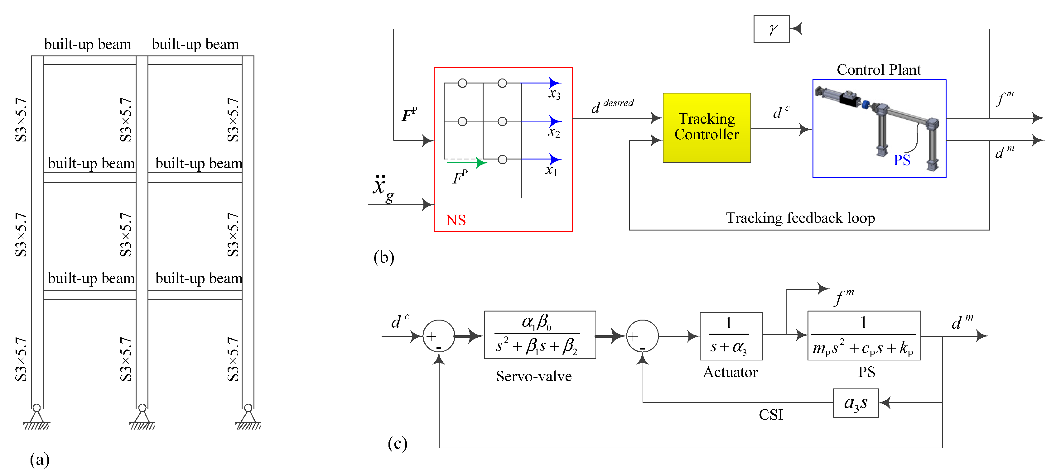
2. Overview of the Benchmark Problem in RTHS

In RTHS, the emulated structure is divided into PS and NS, and they are related by a transfer system. The equation of motion for the NS is

$${\mathrm{M}}_{\mathrm{N}}{\ddot{\mathrm{X}}}_{\mathrm{N}}+{\mathrm{C}}_{\mathrm{N}}{\dot{\mathrm{X}}}_{\mathrm{N}}+{\mathrm{K}}_{\mathrm{N}}{\mathrm{X}}_{\mathrm{N}}+{\mathrm{r}}_{\mathrm{P}}({\mathrm{X}}_{\mathrm{P}},{\dot{\mathrm{X}}}_{\mathrm{P}},{\ddot{\mathrm{X}}}_{\mathrm{P}})=-\mathrm{M}\mathsf{\Gamma }{\ddot{\mathrm{x}}}_{\mathrm{g}}$$

(1)

where M, C, and K are the mass, damping, and stiffness matrices of the structure, respectively; the subscripts “N” and “P” represent the NS and PS, respectively; X denotes the displacement vector of the structure and Γ refers to the location vector; r is the restoring force vector and ${\ddot{\mathrm{x}}}_{\mathrm{g}}$ is the ground acceleration.

Equation (1) is solved by employing a time-stepping integration algorithm, and the calculated displacement X_P is forwarded to the PS to satisfy the compatibility condition using a displacement-control-based actuator. Then, the force at the boundary interface is measured directly and fed back into the NS to satisfy the equilibrium. The above procedure is repeated until the termination condition is reached.

However, owing to the dynamics of the control plant, the boundary conditions of NS and PS are often de-synchronized. Hence, in recent years, numerous approaches have been proposed and examined to treat this issue under certain conditions. To provide a unified performance evaluation standard for different methods and to advance the field of RTHS, a Benchmark problem in RTHS was established by Silva et al. [32]. In the Benchmark problem, the models of the servo-hydraulic transfer system, the sensing and control implementation hardware, control-structure interaction, and the PS are identified from the actual equipment [33] and modeled by transfer functions in MATLAB. The block diagram of the benchmark problem is depicted in Figure 1.

2.1. Reference Model

As illustrated in Figure 1a, the reference structure is a three-story, two-bay moment-resisting steel frame structure. The structure is made from A572 Grade 50 steel, with columns of commercial S3 × 5.7 sections and beams of built-up I sections that are welded by 50 × 6 webs and 38 × 6 flanges. With the assumptions of (1) negligible vertical translations of the nodes, (2) rigid diaphragm, and (3) a lumped mass at the middle of each span, and applying static condensation to the finite-element model, a three degree-of-freedom (DOF) model is reached to represent the reference structure, that is, only the horizontal DOFs are considered in the numerical model. The stiffness matrix of the reference structure is given by K = [2.6055 −2.3134 0.5937; −2.3134 3.2561 −1.4420; 0.5937 −1.4220 0.9267] × 10⁷ N/m. The damping matrix of the reference structure is calculated using modal damping ratios.

2.2. Partitioning Schemes

It has been reported that the partitioning of the reference structure plays a critical role in the successful implementation of the RTHS [34]. The predictive stability indicator (PSI), which is defined as PSI = log₁₀(τ_cr), where τ_cr is the critical time delay, is used to quantify the sensitivity of different partitioning choices to de-synchronization at the interface between the substructures. A smaller value of PSI indicates that the RTHS is more sensitive to the de-synchronization. In the Benchmark problem, four different partitioning schemes were considered with PSI values ranging between 0.6 (moderately sensitive) and 1.05 (slightly sensitive), which is equivalent to τ_cr values between 4 and 11 ms. The four partitioning cases are listed in

Table 1. Partitioning cases.

Partitioning Configuration	Reference Floor Mass (kg)	Reference Modal Damping (%)
Case 1	1000	5
Case 2	1100	4
Case 3	1300	3
Case 4	1000	3

.

The PS is a portal frame that is built in the Intelligent Infrastructure Systems Lab (IISL), as described in Figure 1b. The mass, lateral stiffness, and damping coefficient of the PS are 29.12 kg, 1.19 × 10⁶ N/m, and 114.6 Ns/m, respectively, which were identified using experimental data.

2.3. Control Plant and Control Problem Statement

Figure 1b depicts the model of the control plant, where the dynamics of the servo-valve, actuator, PS, and control-structure interaction (CSI, Dyke et al. [24]) are individually modeled using transfer functions. Specifically, the servo-valve is represented by a second-order transfer function with parameters of α₁ and β₀ to β₂; the dynamics of the hydraulic actuator are modeled by a first-order transfer function with parameters of α₃; the CSI that caused by the natural velocity feedback loop is modeled by the derivative with parameter α₂; the PS is represented by a transfer function with parameters of m_P, c_P, and k_P. The parametric values of the model are identified using experimental data, which are presented in

Table 2. Parametric values of the control plant.

Parameter	Component	Nominal Value	Standard Deviation	Units
α1β0	Servo-valve	2.13 × 1013	-	m·Pa·s−1
α2	CSI	4.23 × 106	-	m Pa
α3	Actuator	3.3	1.3	1/s
β1	Servo-valve	425	3.3	Unitless
β2	Servo-valve	10 × 104	3.3 × 103	1/s
mp	PS	29.12	-	kg
kp	PS	1.19 × 106	5 × 104	N/m
cp	PS	114.6	-	kg/s

. Additionally, to validate the robust stability and performance of the designed controller or compensator, model uncertainties were accounted for using a random variable with a normal distribution of each parameter, and are also given in Table 2. Please note that the control plant assigned with the mean values of each parameter are denoted as a nominal plant, whereas that assigned using parameters that differ from the nominal ones are referred to as a perturbed model.

As a result of series, parallel, and feedback connections of those components, the mathematical control plant model, from command displacement to the measured displacement, is given by

$$G_{\mathrm{CP}}\left(s\right)=\frac{A_0}{B_5{s}^5+B_4{s}^4+B_3{s}^3+B_2{s}^2+B_{1}s+B_0},$$

(2)

where s is the Laplace transform variable, A₀ = α₁β₀, B₅ = m_p, B₄ = c_p + m_pα₃ + m_pβ₁, B₃ = (k_p + c_pα₃ + α₂) + (c_p + m_pα₃)β₁ + m_pβ₂, B₂ = k_pα₃ + (k_p + c_pα₃ + α₂)β₁ + (c_p + m_pα₃)β₂, B₁ = k_pα₃β₁ + (k_p + c_pα₃ + α₂)β₂, B₀ = α₁β₀ + k_pα₃β₂.

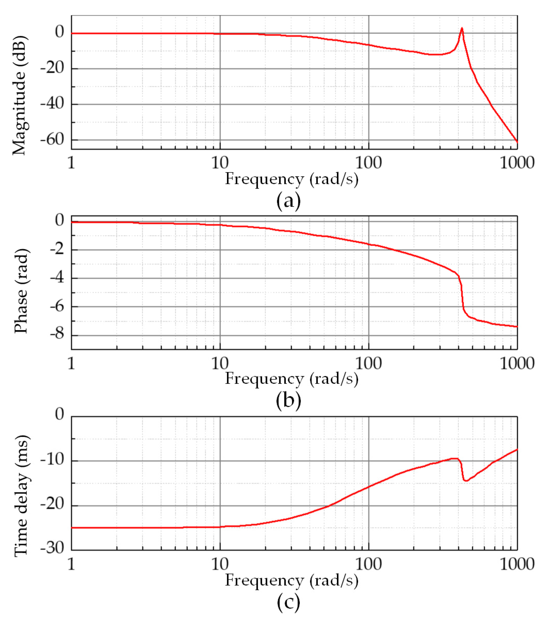
The magnitude, phase, and time delay of the nominal control plant (Equation (2)) are investigated and presented in Figure 2. In the figure, the time delay is evaluated using τ = φ/ω. From Figure 2a,b, it can be observed that when the frequency is low, e.g., the frequency <10 rad/s, both the magnitude and phase are minimal. As the frequency increases, the magnitude decreases while the phase increases, implying that the tracking performance is weakened. Hence, the compatibility and equilibrium cannot be satisfied for all interface boundary DOFs, and the compensation methods for amplitude and phase errors must be employed. Furthermore, the time delay is varying from 25 ms to 8 ms, as shown in Figure 2c. That is, the constant delay-based compensation method may no longer be suitable. Hence, to obtain an accurate RTHS result, the compensation strategy considering the variant time delay and amplitude error must be employed.

2.4. Implementation Constraints

As the control plant model is achieved from the physical devices available in the laboratory, virtual RTHS (vRTHS) must be subjected to the following implementation constraints:

• The compensator has to be in the discrete form.
• The sampling frequency of the vRTHS test is 4096 Hz.
• The servo-hydraulic actuator responses should be within the maximum capacity of 8900 N, a stroke of 7 mm, and a maximum velocity of 25 mm/s.
• The A/D and D/A converters have an 18-bit precision and a span of 3.8 V, and are modeled as a saturation block combined with a quantizer in the Simulink software tool.
• Sensor conversion factors from voltage to displacement in mm and voltage to force in N are considered, and are 7.89 mm/V and 1096 N/V, respectively.
• The measurement noise is considered and modeled as a Gaussian process whose statistics are obtained from experimental observations. The noise level is approximately 0.05% of the full span of the A/D converter.

2.5. Evaluation Criteria

To quantify the performance of the vRTHS, nine evaluation criteria provided in Silva et al. [32] were used in this study. The evaluation criteria J₁ to J₉ are presented in

Table 3. Performance evaluation criteria.

Criterion	Description	Definition	Units
J1	Tracking time delay	$J_1=\underset{k}{\arg \max }\left({\displaystyle \sum _i{d}_i{d}_{i-k}^{\mathrm{m}}}\right)$	ms
J2	Normalized root mean square of the tracking error	$J_2=\sqrt{\frac{{\displaystyle {\sum }_{i=1}^N{(d_i-d_i^{\mathrm{m}})}^2}}{{\displaystyle {\sum }_{i=1}^N{(d_i)}^2}}}\times 100$	%
J3	Peak tracking error	$J_3=\frac{\max \left|d_i-d_i^{\mathrm{m}}\right|}{\max \left|d_i\right|}\times 100$	%
J4	Normalized RMS relative displacement at the first floor	$J_4=\sqrt{\frac{{\displaystyle {\sum }_{i=1}^N{(d_i^{\mathrm{r}1}-d_i^{\mathrm{m}})}^2}}{{\displaystyle {\sum }_{i=1}^N{(d_i^{\mathrm{r}1})}^2}}}\times 100$	%
J5	Normalized RMS relative displacement at the second floor	$J_5=\sqrt{\frac{{\displaystyle {\sum }_{i=1}^N{(d_i^{\mathrm{r}2}-X_i^2)}^2}}{{\displaystyle {\sum }_{i=1}^N{(d_i^{\mathrm{r}2})}^2}}}\times 100$	%
J6	Normalized RMS relative displacement at the third floor	$J_6=\sqrt{\frac{{\displaystyle {\sum }_{i=1}^N{(d_i^{\mathrm{r}3}-X_i^3)}^2}}{{\displaystyle {\sum }_{i=1}^N{(d_i^{\mathrm{r}3})}^2}}}\times 100$	%
J7	Peak relative displacement error corresponding to the first floor	$J_7=\frac{\max \left|d_i^{\mathrm{r}1}-d_i^{\mathrm{m}}\right|}{\max \left|d_i^{\mathrm{r}1}\right|}\times 100$	%
J8	Peak relative displacement error corresponding to the second floor	$J_8=\frac{\max \left|d_i^{\mathrm{r}2}-X_i^2\right|}{\max \left|d_i^{\mathrm{r}2}\right|}\times 100$	%
J9	Peak relative displacement error corresponding to the third floor	$J_9=\frac{\max \left|d_i^{\mathrm{r}3}-X_i^3\right|}{\max \left|d_i^{\mathrm{r}3}\right|}\times 100$	%

. J₁ is the tracking time-delay, assessing the time delay between reference and output signals. J₂ is the root mean square error (RMSE), valuating the tracking error using the normalized root-mean square (RMS). J₃ is a normalized peak tracking error measure. J₄ to J₆ are the normalized RMS errors between the reference and RTHS floor displacements and J₇ to J₉ are the normalized peak tracking errors between the reference and RTHS floor displacements. J₄ to J₉ evaluate the performance of the vRTHS compared to the reference model. It should be noted that in this study, the reference solution is obtained by solving equation of motion employing the explicit fourth-order Runge-Kutta scheme with a fixed time step.

It should be noted that d^rj (j = 1,2,3) is the reference displacement, and X^j (j = 2,3) is the floor displacement of RTHS.

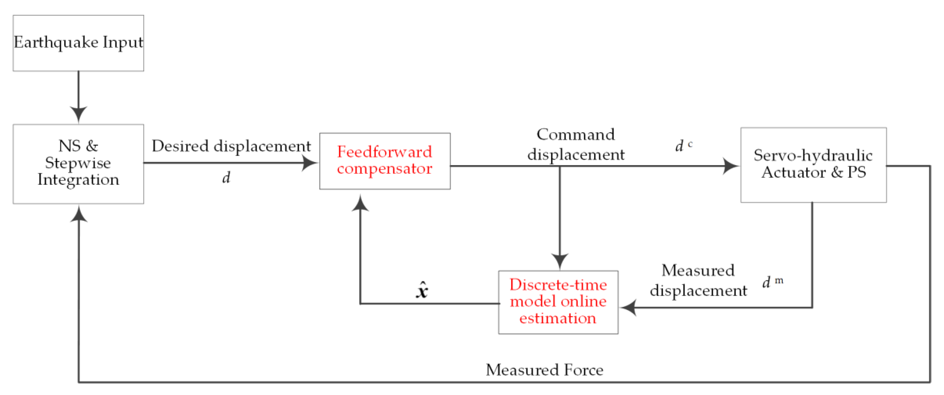
3. Discrete-Time Adaptive Delay Compensator Based on Kalman Filter

To address the variant time delay in RTHS, numerous control strategies have been proposed and validated over the past 20 years. The feedforward-based approaches have received widespread attention for their fast compensation characteristics in terms of phase and amplitude. By taking the inverse of the control plant model as the feedforward controller, the time delay and amplitude discrepancy can be eliminated thoroughly. However, the mathematic model of the control plant is straightly proper, and the feedforward controller thus often consists of an additional low-pass filter and the inverse model of the control plant [35,36], which may cause design difficulties. Concerning adaptive delay compensation methods, their effectiveness largely depends in the performance of the parameter estimation method. This study proposes a KF-based discrete-time adaptive delay compensation (KF-ADC) method, which is an improvement of the general adaptive compensation method proposed by Wang et al. [13]. As shown in Figure 3, the KF-ADC method incorporates two modules, namely the discrete-time model online estimation module and a feedforward controller. Details of the proposed KF-ADC method are presented in this section.

3.1. Discrete Model of Control Plant

Different from the widely investigated adaptive delay compensation methods that employ the inverse of the continuous model of the control plant [19,28,37], this proposed KF-ADC method employs the discrete-time model of the control plant because of its execution convenience on digital signal processing boards. Whether using the Auto-Regressive with Exogenous discrete-time model [38] or transforming the model from the Laplace domain to the time domain, one can always obtain a difference equation description of the control plant by

$$d_k^{\mathrm{c}}={\displaystyle \sum _{i=1}^p{d}_{k-i}^{\mathrm{c}}{x}_i^{\mathrm{c}}+}{\displaystyle \sum _{j=1}^q{d}_{k-j+1}^{\mathrm{m}}{x}_j^{\mathrm{m}}},$$

(3)

where d^c and d^m represent the displacement command and measurement of the control plant, respectively, x is the system model parameter, p and q are two adjustable parameters determined by the orders of the control plant, and the subscript k denotes the k–th time step. Equation (3) can be further reorganized into a more compact form, namely,

$$d_k^{\mathrm{c}}={\mathsf{\phi }}_k^{\mathrm{T}}x,$$

(4a)

where

$${\mathsf{\phi }}_k^{\mathrm{T}}=\left[d_{k-1}^{\mathrm{c}},d_{k-2}^{\mathrm{c}},\cdots ,d_{k-p}^{\mathrm{c}},d_k^{\mathrm{m}},d_{k-1}^{\mathrm{m}},\cdots ,d_{k-q}^{\mathrm{m}}\right],$$

(4b)

$$x={\left[x_1^{\mathrm{c}},x_2^{\mathrm{c}},\cdots ,x_p^{\mathrm{c}},x_1^{\mathrm{m}},x_2^{\mathrm{m}},\cdots ,x_q^{\mathrm{m}}\right]}^{\mathrm{T}}.$$

(4c)

Please note that before establishing this discrete-time model, the orders of the control plant must be determined beforehand.

3.2. Parameter Estimation

Although the mathematical model of the control plant can be established using the first principle modeling method, it is sometimes unable to suitably represent the actual relationship between the displacement command and measurement. Hence, it is necessary to use the actual testing data to revise the system model parameters.

It can be seen that Equation (4a) is a linear difference equation and Ning et al. [31] and Wang et al. [13] employed the least-square method to estimate the system model parameter. However, the convergence of the least-square method cannot be guaranteed, and it is sometimes time consuming. To overcome the previously mentioned problems, a promising estimator, the KF is used to estimate the system model parameter. In this study, the RTHS system is assumed to be a slow time-varying system, and the state and observed equation for this estimation problem can hence be given by

$$x_{k+1}=x_k,$$

(5)

$$y_k=H_k{x}_k+v_k,$$

(6)

where H_k = φ_k^T, y_k is the commanded displacement at the k–th time step, and v is the measurement noise that satisfies

$$\mathrm{E}{v}_k=0,\mathrm{E}{v}_k{v}_k^{\mathrm{T}}=R,$$

(7)

where R is the measurement noise covariance. The KF estimates the system model parameter vector using

$${\widehat{x}}_{k+1}={\widehat{x}}_k+G_k\left(y_k-H_k{\widehat{x}}_k\right),$$

(8)

where $\widehat{x}$ denotes the estimate of x, and G_k is the Kalman gain, which is calculated by

$$G_k=P_{k-1}{H}_k^{\mathrm{T}}{\left(H_k{P}_{k-1}{H}_k^{\mathrm{T}}+R\right)}^{-1},$$

(9)

where P is the estimate error covariance, which is given by

$$P_k=\left(I-G_k{H}_k\right)P_{k-1}.$$

(10)

3.3. Time-Delay Compensator

When forwarding the RTHS by one step, the model of control plant can be represented by

$$d_{k+1}^{\mathrm{c}}={\mathsf{\phi }}_{k+1}^{\mathrm{T}}{x}_{k+1}.$$

(11)

Considering the slow time-varying system assumption in the last subsection, it can be assumed that there are minor changes in the system model parameter between two adjacent time steps. Hence, if the parameter estimation method is convergent, one can substitute x_k+1 by ${\widehat{x}}_k$, namely

$$x_{k+1}={\widehat{x}}_k.$$

(12)

Thus, the commanded displacement can be predicted by substituting Equation (12) into Equation (11) based on known displacements. By driving the loading system using the predicted displacement, the discrepancy between the desired displacement and the measured displacement is minimized, and the measured displacement will be identical to the desired displacement in an ideal situation, i.e.,

$$d_{k+1}^{\mathrm{m}}=d_{k+1},$$

(13)

where d is the desired displacement calculated by a stepwise integration method, such as the central difference method [39]. Therefore, the compensated command displacement can be evaluated by

$$d_{k+1}^{\mathrm{c}}={\mathsf{\phi }}_{k+1}^{\mathrm{T}}{\widehat{x}}_k,$$

(14)

where

$${\mathsf{\phi }}_{k+1}^{\mathrm{T}}=\left[d_k^{\mathrm{c}},\cdots d_{k-p+1}^{\mathrm{c}},d_{k+1}^{},d_k^{\mathrm{m}},\cdots d_{k-q+1}^{\mathrm{m}}\right].$$

(15)

However, owing to the noise in the measured displacement, the estimated parameters may fluctuate significantly, resulting in the compensated displacement command roughly, which is detrimental to RTHS. Moreover, before time step k+1, the measured displacements are assumed to be close to the desired displacements for the compensated RTHS system. Hence, to enhance the robustness of the compensated RTHS system, the desired displacements are used to predict the displacement command, resulting in the feedforward compensator eventually given by

$$d_{k+1}^{\mathrm{c}}={\mathsf{\phi }}_{k+1}^{\mathrm{T}}{\widehat{\mathbf{x}}}_k,$$

(16)

where

$${\phi }_{k+1}^{\mathrm{T}}=\left[d_k^{\mathrm{c}},\cdots d_{k-p+1}^{\mathrm{c}},d_{k+1}^{},d_k^{},\cdots d_{k-q+1}^{}\right].$$

(17)

4. Performance of KF Used for Parameter Estimation in RTHS

As described in the last section, only the parameter estimation method is convergent, and the time delay can be well compensated by the proposed KF-ADC. Moreover, it can be seen from Equations (8)–(10) that the performance of the KF is affected by the measurement noise covariance R and the initial values of x₀ and P₀. Hence, the performance of the KF in RTHS is investigated in this section.

4.1. Convergence of KF

It can be seen in the state equation and observed equation of the parameter estimation problem, namely Equations (5) and (6), that the process noise is absent. Hence, the stability of the KF cannot be proven based on the uniform complete controllability and observability of the line system [40]. Let e_k denote the difference between the estimated parameter and actual value, namely

$$e_k={\widehat{x}}_k-x,$$

(18)

Substituting Equations (6) and (18) into Equation (8), one can obtain the dynamics of the mathematical expectation of the estimation error, i.e.,

$$e_{k+1}=\left(I-G_{k+1}{H}_{k+1}\right)e_k.$$

(19)

Here, defining the Lyapunov function for system Equation (19) as follows,

$$V_k=e_k^{\mathrm{T}}{P}_k^{-1}{e}_k,$$

(20)

then substituting Equations (9), (10), and (19) into Equation (20), the following equation can be obtained.

$$V_k=V_{k-1}-{\left[H_k{e}_{k-1}\right]}^{\mathrm{T}}{\left(H_k{P}_{k-1}{H}_k^T+R\right)}^{-1}\left[H_k{e}_{k-1}\right].$$

(21)

In RTHS, the elements in the observation matrix H_k are measured from the test, and they are varying and linearly independent considering the measurement noise. If H_ke_k-1 = 0 holds for all values of k, one will obtain e_k-1 = 0, namely ${\widehat{x}}_k$ = $x$. If H_ke_k-1≠0, then the Lyapunov function is decreased, and the system of Equation (19) is stable. Furthermore, the spectral radius of the matrix I–G_kH_k is not greater than 1, and is equals to 1 does not hold. Thus, e_k–1→0 as k→∞, namely the estimated parameters by KF can converge to the true value. Hence, the KF is convergent in parameter estimation problems in Section 3.2.

4.2. Tracking Performance with Prescribed Displacement Command

For convenience, the control plant is modeled by a second-order transfer function, which is given by

$$T\left(s\right)=\frac{{\omega }^2}{s^2+2\zeta \omega s+{\omega }^2},$$

(22)

where ω and ζ are the equivalent circular frequency and damping ratio, respectively, and the two parameters are set to be 50 rad/s and 0.8, respectively. By using the forward-difference method in Equation (22), a three-parameter discrete control plant model can be obtained, namely

$$d_{k+1}^{\mathrm{c}}=x_1{d}_{k+1}^{\mathrm{m}}+x_2{d}_k^{\mathrm{m}}+x_3{d}_{k-1}^{\mathrm{m}},$$

(23)

and the corresponding feedforward compensator is given by

$$d_{k+1}^{\mathrm{c}}={\widehat{x}}_1{d}_{k+1}^{}+{\widehat{x}}_2{d}_k^{}+{\widehat{x}}_3{d}_{k-1}^{}.$$

(24)

In this section, the sampling frequency is 4096 Hz, resulting in the true parameters for the three-parameter discrete model of the second-order control plant model in Equation (22) being x_true = [0.6777 −1.3422 0.6646]^T × 10⁴. The initial value of x, which is denoted by x₀, is determined by employing the least-square method, where the displacement command and measurement originated from the control plant without using any compensation method. Thus, the initial value x₀ is [0.5817 −1.152 0.5704]^T × 10⁴. The initial covariance matrix P₀ is assumed to be diagonal, which means that the initial values of the parameters are statistically uncorrelated. The diagonal entries of P₀ are computed as (q_f×x_i)² [41], where i = 1, 2, 3, and q_f = 0.1. The measurement noise R is set to be 0.001. It should be noted that the measurement noise was modeled by the random number, and a KF was used to suppress the effect of noise.

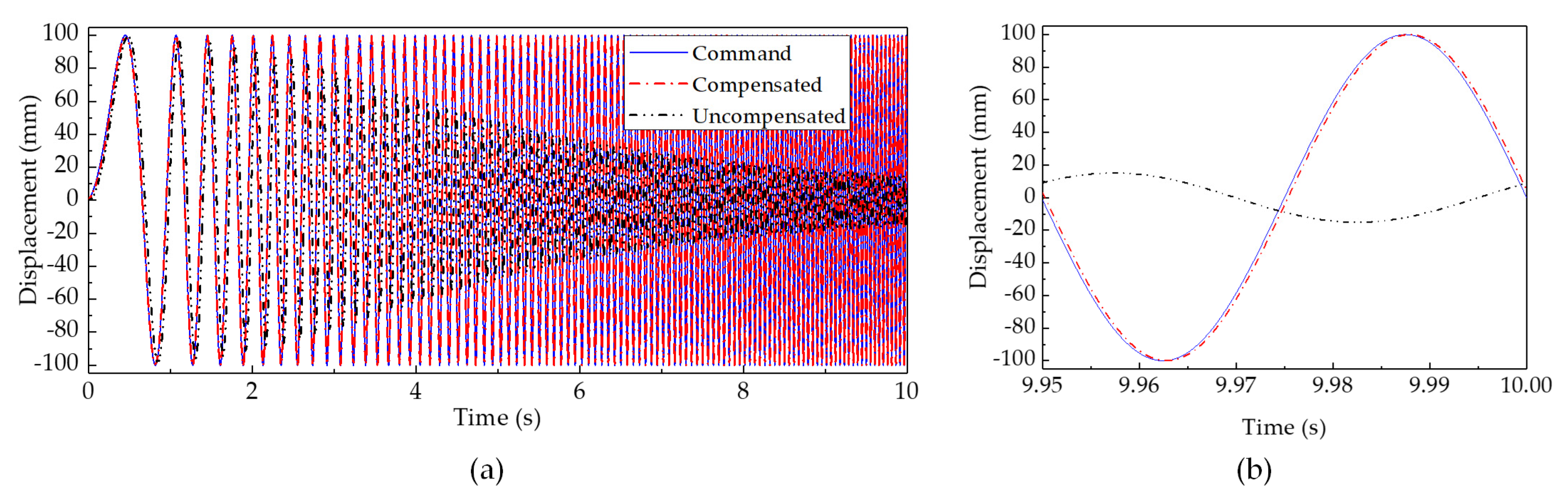
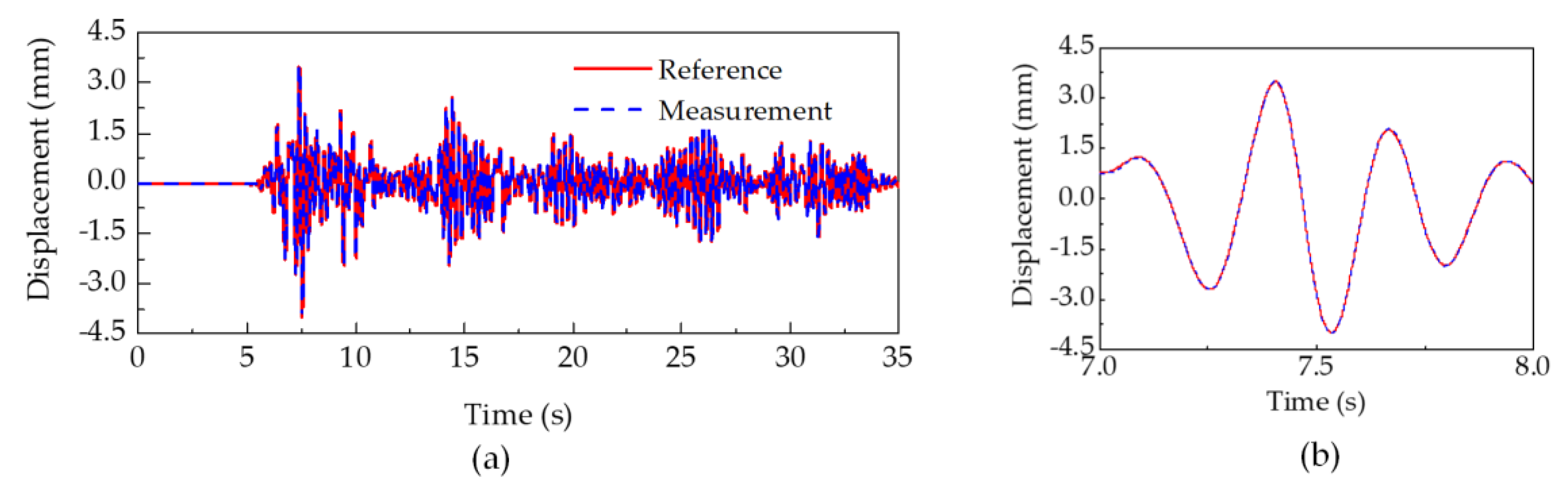
The tracking performance of the second-order transfer system is shown in Figure 4, where the displacement command is a swept signal with frequency ranging from 0.1 Hz to 20 Hz, and has an amplitude of 100 mm. For comparison, the response without any compensation method is also given in the figure. It is seen that as the input frequency increases, the tracking performance without compensation decreases rapidly, which is detrimental to RTHS. On the contrary, it can be found in Figure 4a that the measurement displacement provided by the proposed KF-ADC method agrees well with the displacement command. The enlarged view is shown in Figure 4b, and it can be seen that the measurement displacement is almost identical to the displacement command. This reveals that by compensating using the proposed method, the control plant exhibits a very good tracking performance.

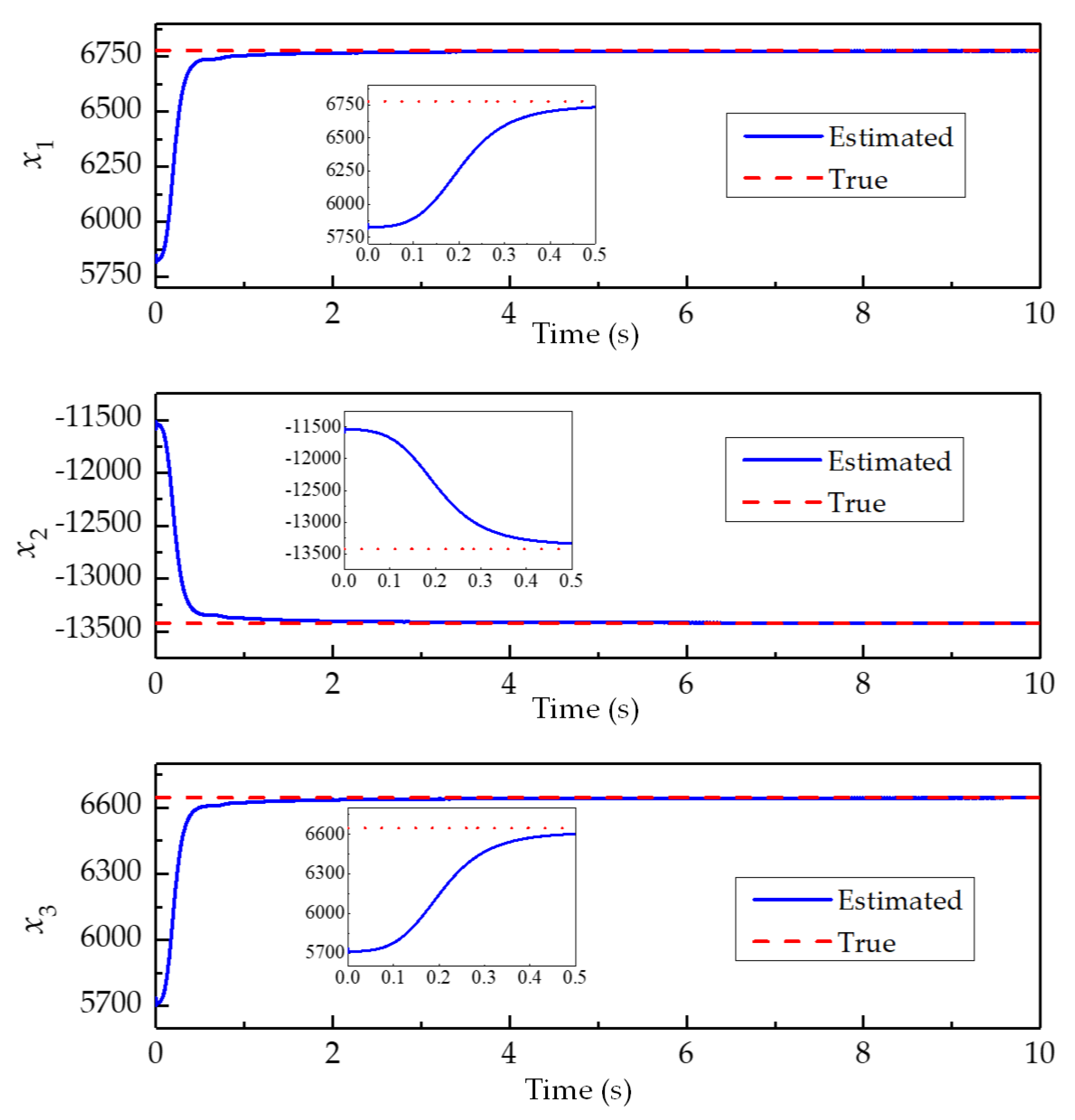
The evolutions of the estimated system model parameter values are shown in Figure 5. It is seen in the figure that the estimated system model parameters vary slightly compared with the initial value after the first 0.1 s. Then, the estimated parameters move rapidly toward the true values between 0.1 s and 0.5 s. Subsequently, the estimated parameters remain relatively stable, and are almost identical to the true ones. This result shows that once the dynamics of the control plant are excited, the discrete-time model of the control plant can be quickly estimated using KFs with high-accuracy, and the time-delay can be compensated effectively. This indicates that the KF has a fast convergence speed and high estimation accuracy.

4.3. Parameter Study of KF

This subsection investigates the influence of the measurement noise covariance R and the initial values of x₀ and P₀ on the proposed time-delay compensation method. To perform this analysis, a series of different values of R, x₀, and P₀ are used. They are considered as Q = W_fQ⁰, where Q represents R, x₀, and P₀, Q⁰ represents the nominal values of R, x₀, and P₀ that were determined in the last subsection, and W_f is a factor varying from 0.7 to 1.3. The duration of the simulations is 10 s, and the stop frequencies of the swept signal are 10 Hz, 20 Hz, and 30 Hz, respectively.

4.3.1. Effect of Initial Guess x₀

The time delay of the control plant compensated by the proposed adaptive delay scheme was calculated and presented in

Table 4. Calculated time-delay.

Wf	Stop Frequency of the Swept Signal
	10 Hz	20 Hz	30 Hz
0.7	0.2	0.2	0.2
0.75	0.2	0.2	0.2
0.8	0.2	0.2	0.2
0.85	0.2	0.2	0.2
0.9	0.2	0.2	0.2
0.95	0.2	0.2	0.2
1	0.2	0.2	0.1
1.05	0.1	0.1	0.1
1.1	0.1	0.1	0.1
1.15	0.1	0.1	0.1
1.2	0.1	0.1	0.1
1.25	0.1	0.1	0.1
1.3	0.1	0.1	0.1

. The table shows that even though the initial guess x₀ varied from −30% to 30%, the calculated time delay of the compensated system remained almost unchanged. Moreover, with the increase in the stop frequency of the swept input signal, the calculated time delay varied over a limited range. For all of the 39 simulations, almost the entire calculated time delay was 0.1 ms, of which the maximum value was 0.2 ms. This indicated that the proposed compensation method is effective and robust.

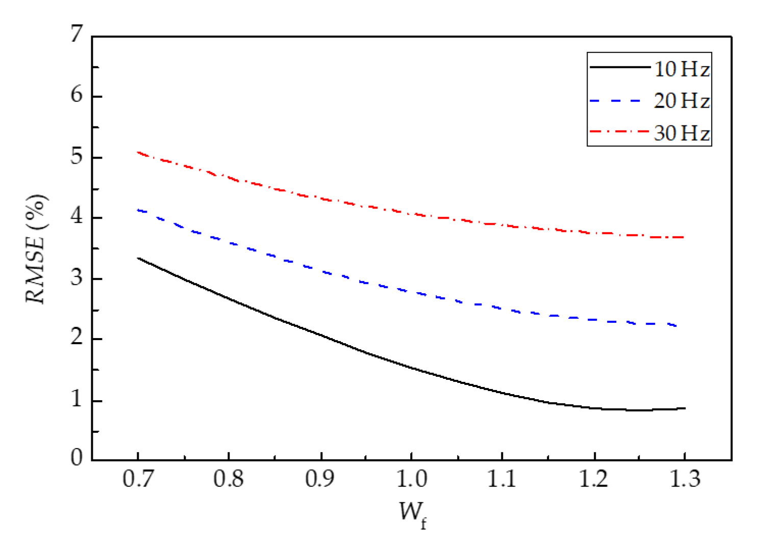
The RMSEs between displacement command and measurement are shown in Figure 6. The figure shows that as the stop frequency increases, the RMSE increases, and the RMSE of the highest stop frequency has the greatest value. Meanwhile, the RMSE decreases first and then increases as W_f increases. Despite this, the maximum value of RMSE is less than 5.0%, indicating that the proposed method is still effective with a different initial guess x₀.

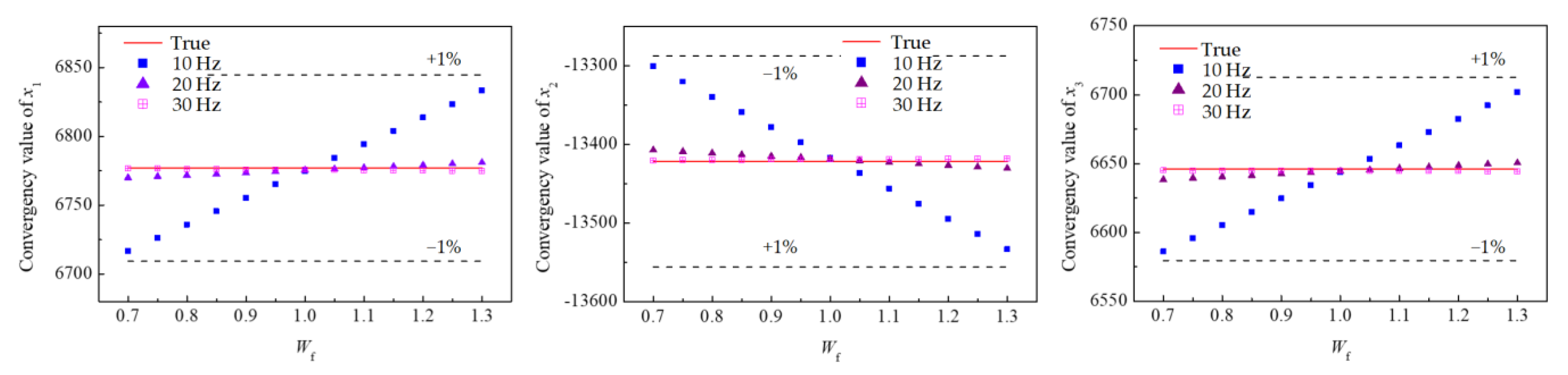
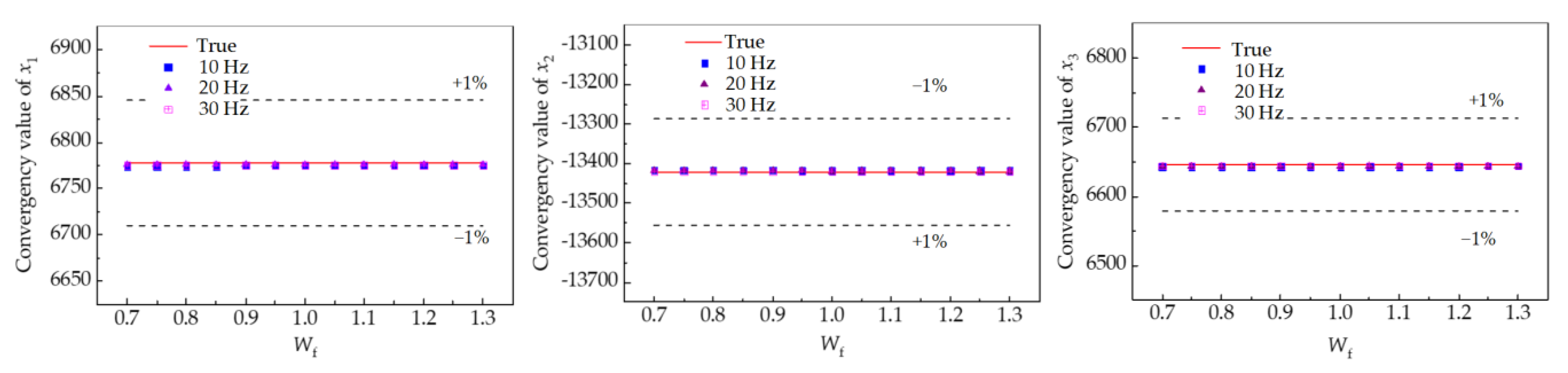
The convergence values for the discrete model are shown in Figure 7. For comparison convenience, the true values and an error threshold of 1% are also given in the figure. The figures show that the converged values remain almost unchanged with an increase in factor W_f. However, if focusing on one of the specifically prescribed displacements, e.g., a stop frequency of 10 Hz, one can find that the converged values increase with an increase in the factor W_f. Furthermore, the relative error between the converged value and the true value is within 1%, indicating that although there are notable errors in the initial value, the parameters of the control plant can also be significantly improved using KF.

4.3.2. Effect of Initial Covariance Matrix P₀ and R

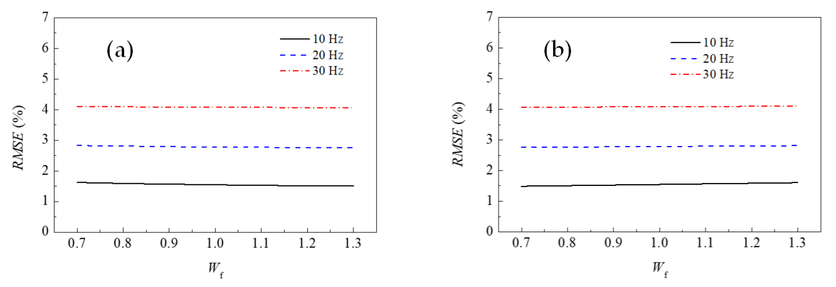
The relationships between the RMSE of the compensated system and the initial covariance and measurement noise covariance are shown in Figure 8. The figures show that for a specific displacement input, as the value of W_f increases, RMSE remains almost the same. Moreover, with an increase in the stop frequency, the RMSE increases. However, the maximum value of the RMSE is less than 5%, indicating that the proposed method is still effective with varying initial guess values.

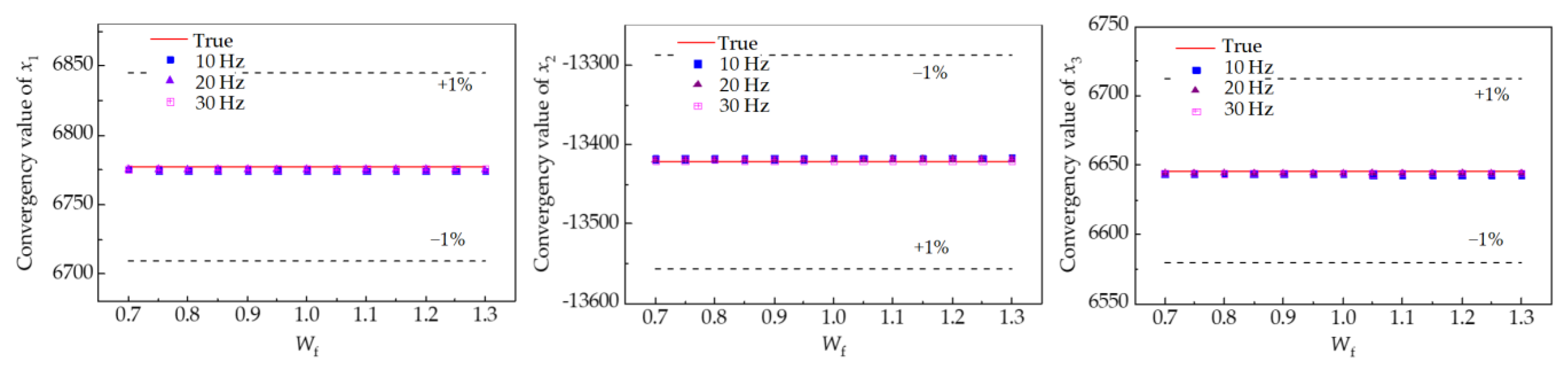
The relationships between the converged value and the factor W_f are shown in Figure 9 and Figure 10. Similar to that used in Figure 7, the true values and the error threshold of 1% are also given in the figure. It can be seen that for all of the considered cases, regardless of which of the three variables changes, i.e., R, P₀, or W_f, the converged value remains at almost the same level. The maximum relative error between the convergency value and the true value is within 1%, indicating that the parameters of the control plant are improved notably, and the parameter estimation method exhibits strong robustness.

5. Numerical Validation

Virtual RTHSs were carried out with three different ground acceleration records, and the four partitioning cases shown in Table 1 were considered for each input. Moreover, one nominal vRTHS and 20 perturbed vRTHSs were included to consider the modeling uncertainties for the control plant in each partitioning configuration. A total of 252 vRTHSs (12 nominal vRTHSs and 240 perturbed vRTHSs) were carried out in this study.

In this section, a four-parameter discrete model of the control plant is adopted, namely

$$d_{k+1}^{\mathrm{c}}=x_1{d}_{k+1}^{\mathrm{m}}+x_2{d}_k^{\mathrm{m}}+x_3{d}_{k-1}^{\mathrm{m}}+x_4{d}_{k-2}^{\mathrm{m}},$$

(25)

and the corresponding feedforward controller is

$$d_{k+1}^{\mathrm{c}}=x_1{d}_{k+1}^{}+x_2{d}_k^{}+x_3{d}_{k-1}^{}+x_4{d}_{k-2}^{}.$$

(26)

To determine the initial values of x₀, P₀, and R, a virtual RTHS (vRTHS) without any compensation strategy was carried out, where the El Centro ground acceleration is scaled to 0.2 g. By employing the least-square method, the initial value x₀ reaches [11.1688 −20.4226 13.6773 −3.4339]^T. The measurement noise variance R is set to 1 × 10^-4, which is determined by the characteristics of the noise level. Similar to that used in the last subsection, the initial covariance matrix is given by P₀ = diag([11.1688² 20.4226² 13.6773² 3.4339²]).

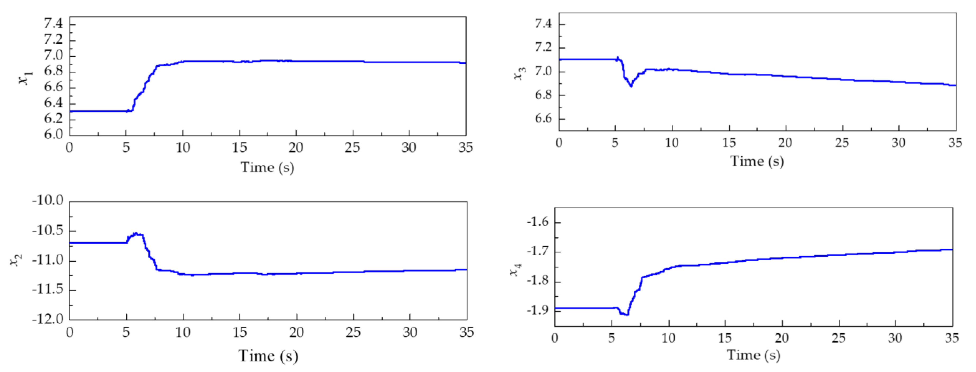
The displacement time history of the first floor from nominal virtual RTHS for Case 1 under the El Centro earthquake record is shown in Figure 11, with the reference response provided. From the figure, it can be seen that the displacement of the virtual RTHS is almost identical to the reference one, which indicates a good tracking performance of the proposed compensation strategy. The evolutions of the estimated system model parameters are given in Figure 12, correspondingly. It can be seen that once the dynamics of the control plant are excited and there are differences between the desired and measurement displacements, the KF responds rapidly to adjust the system model parameter, and then the parameters converge rapidly to a relatively steady value. It may be noted that the convergence trend of x₃ and x₄ is not very evident, but the compensated control plant exhibits a nearly perfect tracking performance, as shown in Figure 11b. This is because the parameters x₃ and x₄ are related to the dynamics of the control plant in the high-frequency range, which are not excited completely. Furthermore, it is seen that there are few large fluctuations during the loading period, implying the stable performance of the parameter estimation method.

The quantitative indicators that were introduced earlier for the nominal vRTHSs under El Centro, Kobe, and Morgan Hill ground motions are presented in

Table 5. vRTHS evaluation criteria for nominal cases.

Earthquake Record	Case	Evaluation Criteria
		J1	J2	J3	J4	J5	J6	J7	J8	J9
El Centro	Case 1	0.20	1.10	1.42	3.77	2.81	3.36	3.37	2.09	2.06
	Case 2	0.20	1.06	1.59	3.51	2.05	3.15	3.17	1.76	1.74
	Case 3	0.20	0.78	1.28	4.50	3.32	4.41	4.41	3.04	3.09
	Case 4	0.20	0.93	1.18	5.70	3.18	5.40	5.42	2.79	2.78
Kobe	Case 1	0.20	1.15	1.24	2.81	1.92	2.52	2.52	1.50	1.50
	Case 2	0.20	1.04	1.15	3.53	2.27	3.35	3.35	1.97	2.00
	Case 3	0.20	1.03	1.17	3.28	2.19	3.23	3.22	1.99	1.99
	Case 4	0.20	1.03	1.20	4.37	2.54	4.23	4.23	2.46	2.46
Mogan Hill	Case 1	0.20	1.20	1.14	3.13	2.69	2.80	2.81	2.29	2.29
	Case 2	0.00	1.19	0.90	2.96	2.29	2.65	2.66	1.72	1.71
	Case 3	0.00	1.12	0.91	3.15	1.75	3.06	3.07	1.61	1.59
	Case 4	0.20	0.93	1.04	4.77	4.13	4.55	4.57	3.91	3.89

. In the table, it is shown that the maximum value of J₁, which is the calculated time delay, is 0.2 ms, which is much less than the critical time delay (approximately 4 ms) in all cases. This indicates that the proposed KF-ADC method is efficient in terms of providing a stable RTHS considering different partitioning schemes. Moreover, the maximum value of J₂ and J₃ is less than 2%, implying that the KF-ADC method also achieves good global agreement between the desired and measured displacements in all cases.

If focusing on the criteria between the results from vRTHS and the reference solution, namely the global errors (J₄, J₅, and J₆) and relative peak errors (J₇, J₈, and J₉), it can be seen that most of them are less than 5%. This demonstrates that the proposed KF-ADC method enables the RTHS to reliably assess the structural performance under different dynamic loads. Furthermore, it can also be observed that with the increase in the sensitivity of different partitioning schemes, both the global errors and relative peak errors generally tend to increase. However, the maximum value of the criteria J₄ to J₉ is still acceptable. This indicates that the proposed KF-ADC strategy enables RTHS to obtain reliable results when the partitioning configuration is in the moderately and slightly sensitive regions.

To further investigate the robustness of the KF-ADC strategy proposed in this study, the mean and standard deviation of the evaluation criteria for the 240 perturbed vRTHSs are shown in

Table 6. Mean of evaluation criteria for perturbed cases.

Earthquake Record	Case	Evaluation Criteria
		J1	J2	J3	J4	J5	J6	J7	J8	J9
El Centro	Case 1	0.42	1.50	2.16	4.90	3.80	4.35	4.37	2.87	2.87
	Case 2	0.20	1.23	1.76	3.40	2.30	2.93	2.94	1.71	1.71
	Case 3	0.27	0.97	1.57	5.23	3.86	5.15	5.15	3.57	3.62
	Case 4	0.30	1.19	1.80	6.59	3.97	6.20	6.22	3.39	3.38
Kobe	Case 1	0.29	1.40	1.41	3.11	2.17	2.77	2.78	1.67	1.66
	Case 2	0.27	1.26	1.30	3.99	2.59	3.75	3.75	2.20	2.21
	Case 3	0.33	1.41	1.63	3.77	2.72	3.77	3.76	2.49	2.48
	Case 4	0.32	1.33	1.43	5.13	2.98	5.00	5.00	2.87	2.87
Mogan Hill	Case 1	0.19	1.58	1.75	3.71	3.19	3.16	3.17	2.61	2.60
	Case 2	0.19	1.48	1.36	3.55	2.64	3.05	3.06	2.02	2.03
	Case 3	0.25	1.50	1.52	4.42	2.81	4.18	4.19	2.23	2.21
	Case 4	0.16	1.15	1.42	5.19	4.49	4.86	4.87	4.13	4.11

and

Table 7. Standard deviation of evaluation criteria for perturbed cases.

Earthquake Record	Case	Evaluation Criteria
		J1	J2	J3	J4	J5	J6	J7	J8	J9
El Centro	Case 1	0.31	0.39	0.66	1.53	0.95	1.57	1.58	1.02	1.03
	Case 2	0.22	0.26	0.49	0.79	0.45	0.88	0.88	0.54	0.53
	Case 3	0.27	0.31	0.58	1.69	1.29	1.80	1.80	1.35	1.36
	Case 4	0.27	0.37	0.68	2.32	1.38	2.27	2.28	1.46	1.47
Kobe	Case 1	0.29	0.30	0.23	0.76	0.48	0.89	0.89	0.46	0.46
	Case 2	0.28	0.29	0.24	1.28	0.65	1.42	1.42	0.81	0.83
	Case 3	0.34	0.33	0.41	1.24	0.63	1.55	1.54	0.92	0.91
	Case 4	0.27	0.31	0.27	1.58	0.82	1.74	1.74	0.98	0.97
Mogan Hill	Case 1	0.29	0.44	0.63	1.76	1.43	1.74	1.75	1.43	1.43
	Case 2	0.24	0.28	0.40	1.56	1.12	1.57	1.58	1.04	1.06
	Case 3	0.32	0.39	0.55	2.24	1.23	2.30	2.30	1.05	1.05
	Case 4	0.19	0.22	0.31	2.33	2.00	2.38	2.39	2.00	2.01

, respectively. By comparing the mean of the nine criteria from the perturbed vRTHSs in Table 6 and those from the nominal vRTHSs in Table 5, similar trends can be observed. The maximum value of the criteria for J₄ to J₉ is less than 15%. Moreover, based on the standard deviation presented in Table 7, the less sensitive partitioning scheme is preferred in order to obtain more robust RTHS results. However, the standard deviation of the evaluation criteria of each partitioning configuration and load case is generally less than 2% and no more than 3%, which demonstrates that the proposed KF-ADC method exhibits good robustness when uncertainties are considered in the control plant.

6. Comparison with Existing Methods

To comprehensively investigate the KF-ADC strategy proposed in this study, several other promising delay compensation methods were employed to provide the reference for evaluating the proposed compensator strategy. These are the widely used proportional integral (PI) control with a phase lead compensator (PI, Silva et al. [32]), the model-based controller (MBC, Phillips and Spencer Jr [19], the adaptive model reference controller (aMRC, Najafi and Spencer [42]), and the tracking error-based adaptive delay compensation method (TE-AC, Tao and Mercan [43]). The simulation results provided in Najafi and Spencer [42] and Tao and Mercan [43] are cited here.

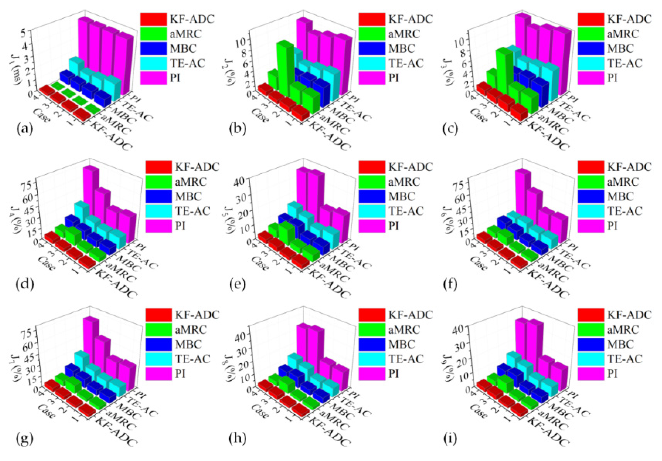
The evaluation criteria for vRTHS employing nominal parameters with different partitioning configurations under the El Centro earthquake are shown in Figure 13. It can be seen in the figure that the nine criteria provided by PI are generally the largest, indicating that the traditional control method may not be very effective to deal with variant time delay in RTHS. With the exception of the tracking criteria of J₂ and J₃, the simulation results generated by aMRC are better than that by MBC, implying that the time delay in RTHS is varying, and constant delay compensation is not sufficient. The aMRC exhibits better performance compared to TE-AC, which is mainly caused by the large number of parameters that should be adjusted in TE-AC.

Furthermore, it can be seen in Figure 13 that the proposed delay compensation scheme is competitive compared with the promising aMRC strategy. With the exception of the calculated time delay of the proposed method is a little larger than that of the aMFC, the other eight evaluation criteria provided by the proposed method are generally smaller, especially for J₂ and J₃. The reason is that the low-pass filter and the reference model in the aMRC strategy should be determined empirically, which are extremely important. In summary, the proposed method is effective and practical for use in RTHS.

7. Conclusions

To deal with the variant time delay caused by the dynamics of control plant in RTHS, a KF-based discrete-time adaptive delay compensation (KF-ADC) method was proposed. Numerical simulations on the Benchmark problem in RTHS were performed to examine the performance of the proposed method. The main conclusions are as follows.

• The principle of the proposed delay compensation method for RTHS was provided. The control plant is represented by a discrete model with time-varying coefficients, which are estimated and updated by KF using the displacement commands and measurements. Based on this model, the compensator is constructed by employing the desired displacements to deal with the variant time delay.
• The performance of the KF used for parameter estimation in RTHS was investigated. By employing the Lyapunov stability theory, it was confirmed that the KF can converge to the true value. Simulations revealed that the KF converged rapidly. When the initial settings of the KF, namely R, x₀, and P₀, varied with 30% of the nominal value, the relative errors of the converged values of the system parameters were less than 1%. It means errors in the initial settings of the KF had a limited effect on the convergent value, and the KF was robust to initial settings.
• The effectiveness of the proposed method was validated through the Benchmark problem in RTHS. The results of 252 vRTHSs revealed a satisfactory tracking performance and robustness of the proposed strategy. Specifically, the maximum value of mean of the estimated time delay was less than 0.5 ms, the maximum value of tracking errors (J₂ and J₃) was less than 2%, and the global errors (J₄, J₅, and J₆) and relative peak errors (J₇, J₈, and J₉) were less than 5%. Moreover, the proposed method was compared with the other four promising schemes. Results revealed that adaptive delay compensations were better than the constant delay-based compensation strategy. The proposed method was competitive compared with the adaptive model reference controller. In general, the proposed method exhibited a superior performance.

Despite the performance of the proposed strategy can be well illustrated by the virtual RTHSs, where the measurement noise, uncertainties of loading system and specimen, real earthquake records and multiple degrees-of-freedom structures are considered, physical tests are also needed to further validate the actual performance. These actual tests are already planned.