Analysis of the Phenomena Causing Weave and Wobble in Two-Wheelers

Abstract

The present work follows in the tracks of previous studies investigating the stability of motorcycles. Two principal oscillation modes of motorcycles are the well-known wobble and weave modes. The research in this field started about fifty years ago and showed how different motorcycle parameters influence the stability of the mentioned modes. However, there is sometimes a minor lack in the physical analysis of why a certain parameter influences the stability. The derived knowledge can be complemented by some mechanical momentum correlations. This work aims to ascertain, in depth, the physical phenomena that stand behind the influence of fork bending compliance on the wobble mode and behind the velocity dependence of the weave damping behaviour. After a summary of the relevant work in this field, this paper presents different rigid body simulation models with increasing complexity and discusses the related eigenvalue analysis and time behaviour. With these models, the mentioned modes are explained and the physical phenomena only partly covered by the literature are shown. Finally, the influence of the rider model on weave and wobble is presented.

1. Introduction

Motorcycle dynamics have always been an extensive research topic due to the complexity and the influence on the riders’ safety. The knowledge used to develop a stable motorcycle chassis comes, to a certain extent, from experience or sensitivity analysis which sometimes lack physical and theoretical understanding of the hidden phenomena. This paper wants to clarify these phenomena, in particular with regard the understanding of the effect of the front fork bending compliance and of the weave damping behaviour with changing speed.

Two of the principal eigenmodes of a motorcycle are known as wobble and weave. The first one includes almost solely the rotation of the front assembly about the steering axis whose frequency is in the range between 7 and 10 $\mathrm{Hz}$ depending on the motorcycle’s parameters [1]; the second one is more complex, and when affected by this mode, the motorcycle shows roll, yaw, steering-head rotation and lateral displacement [2].

The starting point for this work is an observation resulting from the comparison of experience in reality and simulation results. Using the eigenvalue analysis, the earlier motorcycle models, such as the model of Sharp [3] which only includes a tyre model but no compliances, show a stable wobble mode in the lower speed range (up to 80 $\mathrm{k}$$\mathrm{m}$ $\mathrm{h}$⁻¹), and this mode becomes unstable in the higher speed range. However, the experience with a real motorcycle shows an almost opposite behaviour: lower stability (or even instability) at low speed and increasing stability at higher speed. This was demonstrated through measurements on a real motorcycle by Koch [4]. Previous research addressed this apparent incompatibility between simulation and reality, concluding that the front fork bending compliance is a key parameter when studying wobble [5,6,7,8,9], as discussed further in Section 2. Wisselmann [10] conducted an analysis where the motorcycle stiffnesses were progressively eliminated (i.e., set to infinity); in this case also, a remarkable variation in the motorcycle response was shown.

For weave mode, the situation is different: the well-known correlation between eigenmode-damping and speed is also reproduced by models without chassis compliances [2,5,6]. In this case, up to a certain speed, the weave mode becomes more stable with increasing speed. After a tipping point, the stability degenerates again when the speed increases. This behaviour is unexpected, as the increasing gyroscopic moments of the wheel should stabilise the motorcycle, as is the case, for example, with a gyroscope. This is a complex system to analyse because there are many possible gyroscopic moments and their combined influence is not trivial. This peculiar behaviour is further analysed in Section 4.2.

The different models that will be presented within this paper were produced using open source multibody simulation software named “MBSim” (www.mbsim-env.de) which was developed at the Institute of Applied Mechanics of the Technical University of Munich. An introduction [11] on the functionalities of this software is provided. Multibody simulation is common for vehicle dynamics, and was used, for example, by Cossalter in multiple publications [2,5,7,12]. It allows the building of the desired model through a CAD-like interface, by connecting the bodies with joints and assigning them stiffness and damping when needed. The present motorcycle model is described in Section 3.

To summarise, this work deeply investigates the influence of the front fork bending compliance on the wobble mode. Starting from the point reached by previous authors [1,5,6], Section 4.1 provides a different justification for the well-known effect of the fork bending compliance on wobble damping. Moreover, in Section 4.2 the weave mode is further analysed and a possible justification for its damping behaviour is provided. Finally Section 4.3 investigates the influence of the rider on wobbling and weaving.

2. Related Work

Vehicle dynamics is a very popular research topic which features in many books and publications. Most of the literature is focused on four-wheelers; nevertheless, there is also a huge collection of research on two-wheeled vehicles. The different relevant authors are mentioned below.

Back in 1971, Sharp [3] published a paper about the driving stability of two-wheeled vehicles. This research is considered the starting point of the modern motorcycle dynamics. In fact, thanks to a (linearised) tyre model it was possible to detect the wobble mode, which was not present in the even earlier and less complex motorcycle models by Whipple [13] (p. 195).

Cossalter [2] (p. 278) [5] and Spierings [6] presented a solution to overcome the previously mentioned incoherence between reality and rigid model simulations when analysing wobble. A fork bending compliance with a lumped stiffness was added: a revolute joint in the front fork, with its rotating axis (named twist axis [14]) perpendicular to the steering head axis. A certain stiffness and a damping are assigned to this joint. Lumped parameter models are described in [15]. This kind of modelling is also found in other sources, especially when a more complex non-rigid model is developed [16,17,18,19,20,21].

This additional fork bending results in a more realistic wobble-damping characteristic: wobble-instability at low speed and a clear stabilisation when increasing the speed. Cossalter [2] (p. 280) and Spierings [6] explain this change of characteristic with the combination of two opposed effects caused by the fork bending compliance:

• The bending compliance itself reduces the stability.
• The combination of wheel-spin and the rotation around the twist axis produces a gyroscopic moment about the steering axis, leading to stabilisation.

Since the gyroscopic moment is proportional to the speed, the first effect dominates at low speed, causing lower stability in this speed range. The second effect becomes dominant with increasing speed, which explains the restored stability at high speeds. Section 4.1 investigates the influence of the fork bending compliance considering another phenomenon caused by the bending compliance itself.

There are several parameters affecting a motorcycle’s wobble stability; a complete list can be found in [2,3,17,21]. For this work, besides the fork bending compliance, two tyre parameters are of particular importance: the relaxation length and the cornering stiffness. Some research [3,16,17,20] has underlined that a tyre model with cornering stiffness is necessary in order to simulate the wobble mode. This also suggests an important consideration: the principal cause of the wobble is given by the tyre’s response. When the wheel is subject to an outer disturbance steering the wheel itself, the tyre reacts with a side force which, thanks to the mechanical trail, produces an aligning moment around the steering axis. When returning to the equilibrium position, the wheel starts oscillating about the steering axis, thereby triggering the wobble mode [22]. Depending on the speed of the motorcycle, this oscillation will diverge (unstable behaviour) or converge to the equilibrium (stable behaviour).

The other important tyre parameter influencing wobble is the relaxation length [3,13,23]. Several works [3,16,17,20,24] investigated its effect on wobble damping, underlying how the relaxation length destabilises the wobble mode, since it generates a delay between the wheel steering and the tyre-lateral force generation. As a consequence, Sharp [3] (p. 323) clarifies that both tyre sideslip and tyre relaxation properties are fundamental for a proper representation of a motorcycle’s dynamic properties. Like most of the tyre parameters, the relaxation length also depends on several factors. Pacejka et al. [25] and Sharp [1] report that the relaxation length increases with increasing speed. Moreover, a dependence on the vertical load is present. A more recent paper by Sharp [12] proposes a tyre model based on the Pacejka magic formula [26] where dependencies on both speed and vertical load are reproduced. This model and the related parameters are also used in the present work.

In summary, some minimal requisites for a correct analysis of the wobble mode can be defined. Pacejka [26] and Doria [16] suggest that the tyre properties have the greatest influence on motorcycle stability. The Pacejka magic formula [26] coupled with a first order dynamic response, as described in the previous paragraph, is necessary in order to produce reliable wobble stability analyses [13] (p. 324). This tyre model allows an accurate description of the tyre forces and moments if the frequency of the external forces is lower than 15 $\mathrm{Hz}$ [13]; these conditions are generally satisfied for common stability analysis, therefore the magic formula is used in almost all the latest researches based on multibody analysis [2,7,12,27,28,29]. In addition to the tyre modelling, the lateral compliance at the front of the machine is necessary when simulating wobble [13,30]. This can be obtained with a bending compliance of the front fork [5,6,7,8,9], or by adding a lumped torsional stiffness of the main frame at the steering head joint with its rotation axis perpendicular to the steering axis [12,26,27,28]; a combination of both stiffnesses can also be implemented, as in the present work.

Besides the wobble mode, many of the mentioned sources also analyse vehicle “weave” [2,3,5,6,7,17,19,21]. The weave mode can also be qualitatively represented with a motorcycle model having no flexibilities [13] (p. 195). However, the literature underlines that some additional degrees of freedom (DoF) notably influence the weave mode. In particular, Doria [17] (p. 17) and Splerings [6] (p. 28) underline that the fork bending compliance destabilises the weave mode. Taraborrelli [23] and Cossalter [7] analyse the effect of the swingarm torsional and bending compliance. Reference [23] simulated two motorcycle types with significantly different stiffness values: a super-sport motorcycle (higher stiffness), where the two swingarm compliances had almost no influence on weave, and an enduro-motorcycle, where the swingarm bending compliance slightly destabilised the weave mode, which was at the same time slightly stabilised by the torsional compliance of the swingarm. The results of [7], on the contrary, show the destabilising effect of both swingarm bending and torsional compliance; however, the influence was also small in this case.

Furthermore, the rider has proven to greatly affect the motorcycle’s stability behaviour. In fact, Roe [31] points out that the stability analysis of a riderless motorcycle can be very misleading. Significant changes in the weave stability due to the rider have also been reported by Pacejka [26] (p. 535). The modelling of the rider’s passive response and its influence on stability is a broad topic which will be summarised in Section 3.3 and Section 4.3.

An interesting argument strictly connected to weave is the so called “cornering weave”. During cornering, the in-plane eigenmodes (bounce, pitch) become increasingly coupled with the out-of-plane eigenmodes (weave, wobble), whereby the former shows degrees of freedom typical of the latter and vice versa [9,13,32]. Concerning cornering weave, the eigenvector also shows front and rear suspension travels which are not present in the straight-running weave [32]. This mode-coupling is critical because it provides a signal transmission path from road undulations to lateral motions [33]. Moreover, under cornering conditions, bounce and weave have similar eigenfrequencies in the middle to high speed range (70–120 $\mathrm{k}$$\mathrm{m}$ $\mathrm{h}$⁻¹) [9,24,32,34], thereby leading to mutual triggering [13,33,34]. From these considerations it should be clear that the suspension system must also be modelled when carrying out stability analysis of motorcycles under cornering conditions [13,34].

As mentioned in the introduction, the models for the present work were implemented with the “MBSim” multibody simulation software. Two interesting references in this field are the works of moreCossalter [29] and moreLot [35]. They did not use the same software, but developed two multibody-simulation tools that follow the same principle; they are both based on the symbolic calculation software “Maple” with the second one using a build-in library for multibody modelling called “MBSymba”. These references underline the suitability of a multibody simulation tool for the dynamics and stability analysis of motorcycles. Another piece of software used in several works [12,27,36] is “Autosim”; in this case as well, the authors demonstrated the great advantages provided by multibody modelling when conducting both time and frequency analyses. Following this established research, this modelling and calculation method were chosen for the present work.

3. Modelling

Different models have been developed during the last 70–80 years. Their complexity is obviously related to the objectives they pursue. For example, the wobble has been simulated studying systems capable of shimmy behaviour [37] (p. 166). Limebeer [13] (p. 184) derived the equations of motion of such a system, which possesses two DoF:

• Rotation about the steering axis (in this case perpendicular to the ground).
• Lateral translation of the steering joint used to reproduce lateral flexibility.

The model does not take into account the gyroscopic influences. A liner model with relaxation effect is used for the tyre forces. Even with this strongly simplified configuration, some important effects are described, which also occur in motorcycle modelling. The destabilising effect of the cornering stiffness, as prescribed by Sharp [3], is reproduced. Moreover, the inversion of behaviour experienced in motorcycle simulation when using an infinite stiff front frame (Section 2) is also present. This is a remarkable result, as this model does not reproduce the gyroscopic moments, which are considered in [2,6] as responsible for the inversion of behaviour. This could suggest that also other phenomena influence the wobble stability. In Section 4.1 this hypothesis is further developed.

Limebeer [13] (p. 189) carries on his analysis by converting the shimmy model into a front fork model. In this case, the caster angle is considered for the steering axis and the gyroscopic effects are also considered. Another important feature is a revolute joint connecting the fork assembly to the ground. This simulates the motorcycle’s frame torsional flexibility, which provides a lateral flexibility at wheel level, as described in Section 2. Thanks to this feature, the eigenvalue analysis of this system provides results similar to those generally obtained with motorcycle modelling. Cossalter [2] (p. 251) also produced a similar model with the aim of studying wobble; however, it lacks the mentioned lateral flexibility and transient tyre properties, thereby failing to capture the physics of the wobble mode.

The simplified front fork model is acceptable when the aim is to only reproduce wobble. When studying weave, however, a whole motorcycle model is needed. The "basic" motorcycle model is generally updated with some additional degrees of freedom in order to reproduce, for example, the frame compliance or the rider motion.

In Section 3.1 the motorcycle model used in the present work is explained.

3.1. Motorcycle Model

The model used in this work is based on [10], where a model for BMW sport motorcycles from the 1990s was developed and validated with several experimental data, especially regarding the weave and wobble modes. The kinematic structure of the rear suspension and the dataset in the present paper are based on [12]. This reference uses a model with 13 DoF:

• Six DoF related to the main frame rigid body motion: translation about $x,y,z$ axes, roll ($\rho$), pitch ($\varphi$) and yaw ($\psi$).
• Two wheel spins (${\theta }_{\mathrm{fw}},{\theta }_{\mathrm{rw}}$).
• Two suspension travels ($z_{\mathrm{f}},z_{\mathrm{r}}$).
• Steer rotation ($\delta$).
• Frame torsion (${\alpha }_{\mathrm{fr}}$) at the steering head joint, simulated with a revolute joint with rotation axis perpendicular to the steering axis.
• Rider lean (${\alpha }_{\mathrm{ri}}$) simulated with a revolute joint between the rider’s lower and upper body with rotation axis parallel to the main frame x axis.

In the present work some additional DoF are added, which are shown in Figure 1.

• Three compliances of the front fork, simulated with three revolute joints placed approximately at the half of fork length:

  –

  Bending about the x axis (${\alpha }_{\mathrm{ff}}$); the rotation axis of the revolute joint is perpendicular to the steering axis. This compliance is particularly important for wobble, as explained in Section 2. It allows a lateral motion of the wheel along the y axis.

  –

  Bending about the y axis (${\beta }_{\mathrm{ff}}$); the rotation axis of the revolute joint is parallel to the front wheel axis. This flexibility allows a translation of the wheel along the x axis.

  –

  Torsion (${\gamma }_{\mathrm{ff}}$); the rotation axis of the revolute joint is parallel to the steering axis.

• Lateral motion of the rider’s lower body with respect to the saddle ($y_{\mathrm{ri}}$), simulated with a linear joint with axis parallel to the main frame y axis.
• Rider yaw rotation (${\gamma }_{\mathrm{ri}}$) simulated with a revolute joint between the rider’s lower and upper body with rotation axis parallel to the main frame z axis.
• Swingarm torsion (${\alpha }_{\mathrm{sw}}$), simulated with a revolute joint at the swingarm anchor point with rotation axis parallel to the main frame x axis.

The motorcycle parameters in [12] were obtained through experimental measurements or through estimates. However, some parameter variations have been used in the present work:

• The data for the rider’s upper body mass and inertia tensor were taken from [12]. In [12] the mass and inertia tensor of the rider’s lower body and of the motorcycle’s main frame were fused together. In the present work, with the aim of allowing lateral translation of the rider’s hip (considered as lower body in the present work), the mass and inertia tensor of the main frame in [12] were split between hip and main frame, while ascertaining that the combined inertia tensor and the overall centre of gravity remain unchanged. The data for hip’s mass and inertia tensor were taken from [38]. According to these data, the mass and inertia tensor of the main frame were properly modified. In particular, the hip mass was subtracted from the main frame mass in [12]. Moreover, as explained above, the inertia tensor of the main frame was adapted so that the whole inertia tensor of the lower body and main frame together was equal to the main frame inertia in [12]. The rider’s legs were considered fixed to the main frame, so their mass and inertia were included in it. As reported in [12] (p. 252), the rider’s total mass was 72 $\mathrm{k}\mathrm{g}$.
• In the year of publication of [12] the experimental data of the front fork were not completely available. Some of them were judged by the authors of the present work as not realistic (for example, the mass of the lower fork and its lacking inertia tensor). For this reason, the front fork mass and inertia data were taken from [39], while retaining the overall geometry given in [12].

The motorcycle’s parameters are reported in Appendix A.

The tyre forces and moments were reproduced with the Pacejka magic formula; further details on the tyre model are given in Section 3.4. The software for the motorcycle model is available on GitHub: https://github.com/TUMFTM/motorcycle_model.git.

3.2. Suspension

There are several types of motorcycle suspension. The simplest configuration is composed of a telescopic front suspension and a cantilever rear suspension. However, multi-link suspensions have been developed for both front and rear wheels. For the rear suspension, the multi-link solution allows a non-linear damping curve to be obtained even with a linear damper, as the kinematic function of the damper travel can be adjusted using a rocker. Multi-link at the front suspension generally increases the fork stiffness and favours the anti-dive property. For further details the reader is referred to [13] (p. 327). The motorcycle adopted in the present work uses a telescopic front suspension and a unitrack-like rear suspension (definition of [13]), where the spring-damper unit is connected to the chassis and to a rocker, while a pull rod connects the rocker to the swingarm. The kinematic functions of this rear suspension are presented in [12]. Figure 1 shows its geometry.

3.3. Rider Model

In contrast to cars, the rider’s weight strongly influences the total motorcycle weight in riding conditions. Moreover, the rider has some relative motions with respect to the motorcycle. One can therefore expect the rider to have a great influence on motorcycle stability. This is indeed the case, as shown by both simulation [7,40] and experimental [41] results. In this work we only focus on the rider’s passive motions. This is reasonable, as the eigenfrequencies of wobble and weave are too high for the rider to actively counteract them; therefore, it can be assumed that the rider behaves as a passive body when the motorcycle experiences wobble or weave. Under this assumption, different rider models can be developed. The most simple model has been adopted by several works [12,26,27,28] and includes only one DoF: the rider’s upper body rotation about an axis parallel to the frame x axis. A different one-DoF model [42] reproduces the rider’s rotation about the vertical axis (parallel to the frame z axis); moreover, the connection between the upper body and handlebar is included with a parallel rotational spring-damper element. A 2-DoF model can then be obtained by combining the two previously described models [40]. Finally, the lateral displacement (frame y axis) of the rider’s hip can be added, thereby obtaining a 3-DoF rider model [7]. An interesting observation is made by Limebeer [13] (p. 326) about the influence of the rider’s parameters: he reports that the rider’s upper body parameters mainly influence the weave mode, while the lower body parameters have a greater effect on wobble. The literature also offers several examples of more complex rider models containing up to 28 DoF [43]. In this case, the rider model was used to faithfully evaluate the motorcycle race performances, so that the whole rider motion was needed, including his control action on the handlebars and his lean-in strategy. As introduced at the beginning of this paragraph, the current work pursues a very different objective, i.e., the analysis of the motorcycle eigenmodes, so that such a complex rider model is not necessary and would only complicate the interpretation of the results.

The rider model used in the present work is based on that presented in [7]. The rider is composed by two masses, representing the upper and lower body. The DoF are:

• ${\alpha }_{\mathrm{ri}}$: the rider’s upper body lean.
• ${\gamma }_{\mathrm{ri}}$: the rider’s upper body yaw.
• $y_{\mathrm{ri}}$: the rider’s hip (lower body) lateral motion.

As previously said, the connection with the handlebar is modelled by a rotational spring-damper element which reacts to the relative rotation between the upper body and handlebar, and applies equal and opposite moments for lower body and upper body, and frame and steering head, respectively.

3.4. Tyre Model

As introduced in Section 2, the present model uses the Pacejka magic formula to describe the tyre forces. The tyre model is analogous to that reported by Sharp [12] and is suited for motorcycles, as it accounts for the lateral force generation due to the wheel roll angle (camber angle). Moreover, it also describes the longitudinal forces, thereby allowing the motorcycle to be simulated in all possible conditions. Another peculiar factor is the description of the combined longitudinal and lateral force generation. This means that the maximal tyre-lateral force is reduced when the tyre simultaneously generates a longitudinal force (and vice versa). The model also takes into account the variation of the tyre potential with changing vertical load.

The present tyre model considers the tyre width. In this way, in contrast to thin disc models, the overturning moment must not be added separately, as the lateral migration of the contact point automatically generates this overturning moment [12,28].

The magic formula needs some inputs: longitudinal slip ($\kappa$), slip angle ($\alpha$), camber angle (${\rho }_{\mathrm{w}}$), vertical load ($F_z$). $\kappa$ can be calculated with Equation (1).

$$\kappa =-\frac{v_{x_{\mathrm{C}}}-{\omega }_y(r_{\mathrm{rim}}+r_{\mathrm{c}}cos{\rho }_{\mathrm{w}})}{v_{x_{\mathrm{C}}}},$$

(1)

where $v_{x_{\mathrm{C}}}$ is the longitudinal velocity of the tyre contact point, $r_{\mathrm{rim}}$ is the rim radius, $r_{\mathrm{c}}$ is the tyre crown radius and ${\omega }_y$ is the wheel rotation speed. $\alpha$ is calculated with a first order relaxation equation:

$$\frac{\sigma }{v_{x_{\mathrm{C}}}}\dot{\alpha }+\alpha ={\alpha }_{\mathrm{ss}},{\alpha }_{\mathrm{ss}}=-arctan\left(\frac{v_{y_{\mathrm{C}}}}{v_{x_{\mathrm{C}}}}\right),$$

(2)

where ${\alpha }_{\mathrm{ss}}$ is the slip angle in steady-state conditions, while $v_{y_{\mathrm{C}}}$ is the lateral velocity of the tyre contact point. This means that the lateral force due to the slip angle is generated with some delay depending on the relaxation length $\sigma$. Its value is not constant and depends on both longitudinal speed and vertical load; these dependencies are taken into account in the present model. The longitudinal force and the lateral force due to the camber angle are assumed to build up instantaneously, so no relaxation equation is used.

At this point, a geometrical model of the tyre contact point and a related reference frame are needed in order to calculate the velocity components $v_{y_{\mathrm{C}}},v_{x_{\mathrm{C}}}$ at the contact point itself and the vertical load $F_z$. Firstly, the orientation of the reference frame at the contact point has to be obtained. It should satisfy the following requirements: z axis being perpendicular to the road; x axis being in the wheel plane and parallel to the road. Such a reference frame can be derived with two rotations starting from the reference frame of the wheel carrier, indicated in the following with the subscript Wc. The intermediate reference frame W is obtained as follows:

$$\begin{array}{cc}\hfill {}_{\mathrm{W}}{\mathit{e}}_x& =\frac{{}_{\mathrm{Wc}}{\mathit{e}}_y\times {}_{\mathrm{I}}{\mathit{e}}_z}{{|}_{\mathrm{Wc}}{\mathit{e}}_y\times {}_{\mathrm{I}}{\mathit{e}}_z|},\hfill \\ \hfill {}_{\mathrm{W}}{\mathit{e}}_y& ={}_{\mathrm{Wc}}{\mathit{e}}_y,\hfill \\ \hfill {}_{\mathrm{W}}{\mathit{e}}_z& ={}_{\mathrm{W}}{\mathit{e}}_x\times {}_{\mathrm{W}}{\mathit{e}}_y,\hfill \end{array}$$

(3)

where ${}_{\mathrm{ref}}{\mathit{e}}_i$ is the unit vector of the $i$th axis of the reference frame named “ref”, and ${}_{\mathrm{I}}{\mathit{e}}_z={[0,0,1]}^{\mathrm{T}}$. The frame W has the x axis parallel to the ground. In order to get C, another transformation is needed, which allows the z axis to be perpendicular to the ground:

$$\begin{array}{cc}\hfill {}_{\mathrm{C}}{\mathit{e}}_x& ={}_{\mathrm{W}}{\mathit{e}}_x,\hfill \\ \hfill {}_{\mathrm{C}}{\mathit{e}}_z& ={}_{\mathrm{I}}{\mathit{e}}_z,\hfill \\ \hfill {}_{\mathrm{C}}{\mathit{e}}_y& ={}_{\mathrm{C}}{\mathit{e}}_z\times {}_{\mathrm{C}}{\mathit{e}}_x.\hfill \end{array}$$

(4)

The unit vectors in Equation (3) define the rotation matrix ${}_{\mathrm{I}}{\mathbf{S}}_{\mathrm{W}}={[}_{\mathrm{W}}{\mathit{e}}_x,{}_{\mathrm{W}}{\mathit{e}}_y,{}_{\mathrm{W}}{\mathit{e}}_z]$ from frame W to the inertial frame I. Similarly, the rotation matrix from frame C to I is defined as ${}_{\mathrm{I}}{\mathbf{S}}_{\mathrm{C}}={[}_{\mathrm{C}}{\mathit{e}}_x,{}_{\mathrm{C}}{\mathit{e}}_y,{}_{\mathrm{C}}{\mathit{e}}_z]$. Now the longitudinal and lateral velocities $v_{x_{\mathrm{C}}},v_{y_{\mathrm{C}}}$ can be calculated in the following steps:

$$\begin{array}{cc}\hfill {}_{\mathrm{W}}{\mathit{v}}_{\mathrm{Wc}}& ={}_{\mathrm{I}}{\mathbf{S}}_{\mathrm{W}}^{\mathrm{T}}{}_{\mathrm{I}}{\mathit{v}}_{\mathrm{Wc}},\hfill \\ \hfill {}_{\mathrm{W}}{\mathit{v}}_{\mathrm{C}}& ={}_{\mathrm{W}}{\mathit{v}}_{\mathrm{Wc}}+{}_{\mathrm{W}}{\mathit{\omega }}_{\mathrm{Wc}}\times {[0,-r_{\mathrm{c}}sin{\rho }_{\mathrm{w}},-r_{\mathrm{rim}}-r_{\mathrm{c}}cos{\rho }_{\mathrm{w}}]}^{\mathrm{T}},\hfill \\ \hfill {}_{\mathrm{I}}{\mathit{v}}_{\mathrm{C}}& ={}_{\mathrm{I}}{\mathbf{S}}_{\mathrm{W}}{}_{\mathrm{W}}{\mathit{v}}_{\mathrm{C}},\hfill \\ \hfill {}_{\mathrm{C}}{\mathit{v}}_{\mathrm{C}}& ={}_{\mathrm{I}}{\mathbf{S}}_{\mathrm{C}}^{\mathrm{T}}{}_{\mathrm{I}}{\mathit{v}}_{\mathrm{C}}.\hfill \end{array}$$

(5)

${}_{\mathrm{B}}{\mathit{v}}_{\mathrm{A}}$ is the absolute velocity vector of the generic point A in the generic frame B. The vector ${}_{\mathrm{C}}{\mathit{v}}_{\mathrm{C}}$ represents the velocity of the contact point in frame C; its first and second components provide $v_{x_{\mathrm{C}}},v_{y_{\mathrm{C}}}$.

The last remaining input for the magic formula is the vertical load. This is composed by a constant $F_{z,\mathrm{stat}}$ and a varying part $F_{z,\mathrm{dyn}}$. The constant one is obtained in static equilibrium conditions. The second one depends on motorcycle trim and can be calculated using the tyre carcass compression $\Delta z_{\mathrm{tyre}}$ from the nominal state.

$$\Delta z_{\mathrm{tyre}}=-r_{\mathrm{rim}}cos{\rho }_{\mathrm{w}}-r_{\mathrm{c}}+{}_{\mathrm{I}}z{0}_{\mathrm{C}}-{}_{\mathrm{I}}{z}_{\mathrm{Wc}}.$$

(6)

${}_{\mathrm{I}}z{0}_{\mathrm{C}}>0$ is the vertical distance under static equilibrium conditions between the origin of the inertial frame I and the contact point. ${}_{\mathrm{I}}{z}_{\mathrm{Wc}}>0$ is the instantaneous vertical distance between the origin of the inertial frame I and the wheel carrier Wc. Finally, the tyre vertical load $F_z$ is calculated as follows:

$$F_z=F_{z,\mathrm{stat}}+F_{z,\mathrm{dyn}}=F_{z,\mathrm{stat}}-c_z\Delta z_{\mathrm{tyre}}-d_z{v}_{z_{\mathrm{C}}}.$$

(7)

$c_z,d_z$ are the tyre vertical stiffness and damping, respectively. It is worth pointing out that $\Delta z_{\mathrm{tyre}}$ is negative when the carcass is compressed; therefore, the carcass compression leads, through Equation (7), to an increased vertical load.

All the inputs for the magic formula are now available. The equations of the magic formula are taken from [12], so they are not repeated here. The outputs are: longitudinal force, lateral force and aligning moment. These outputs are applied in the wheel carrier and not at the contact point as in [12]. This choice was made because in MBSim the forces must be applied to a body, which would require the definition of a body in the contact point, which in the actual model structure is not an easy task. Shifting the tyre forces in the wheel carrier requires applying additional moments; this is, however, easily done, as all the lever arms are known or can be derived with geometric reasoning. The equivalence between this force system and the one with the forces applied at the contact point has been verified on a simplified model with a single wheel. The results are equivalent, thereby confirming the correctness of the choice made.

3.5. Validation

As explained in Section 3.1, the motorcycle model in the present work is based on the data of [12]. The obvious solution is then to validate the present model against this reference by Sharp. In order to do so, the front fork data were set to the values in [12]; moreover, the additional DoF were "switched off." This was possible thanks to a functionality developed for this purpose in MBSim, which allows the selection of the DoF to be considered. Reference [12] reports the simulation results of a steady-state cornering condition with fixed roll angle and at different speeds. Several variables are then shown under this condition; particularly important for steady-state cornering are: steering torque, front and rear tyre-lateral forces and aligning moments. The same condition has been tested in the present work and the variables compared. The accordance is very good, with deviations less than 5% for all values. This is shown Figure 2, where $F_{y_{\mathrm{f}}},F_{y_{\mathrm{r}}}$ are the front and rear tyre-lateral forces, while $M_{z_{\mathrm{f}}},M_{z_{\mathrm{r}}}$ are the front and rear tyre aligning moments and $T_{\delta }$ is the steer torque.

As further validation, the present model was also compared with that in [26] (p. 508) by Pacejka. This model renounces some DoF with respect to [12]: the suspensions are not modelled. Moreover, the frame torsional stiffness is not present, while the front fork has bending compliance. Using the same data of [26] and with the same DoF, a comparison of the eigenvalue analysis has been carried out. Additionally, in this case the agreement of the results is very good, with the curves of the wobble and weave eigenfrequencies and damping as a function of the speed almost overlapping, as shown in Figure 3. In this figure, the frequency is expressed in $\mathrm{rad}$ $\mathrm{s}$⁻¹ in order to facilitate the comparison with the results of [26], where this unit of measurement is used. In the subsequent paragraphs, however, the frequency will be expressed in $\mathrm{Hz}$. Additionally, the selection of the speed range in Figure 3 was made according to [26].

4. Results

This section shows the eigenvalue analysis and the time response for the presented model. Starting from these plots, some physical relations will be derived and will help to understand the important phenomena influencing the behaviour of the wobble and weave eigenmodes as a function of vehicle speed.

4.1. Wobble

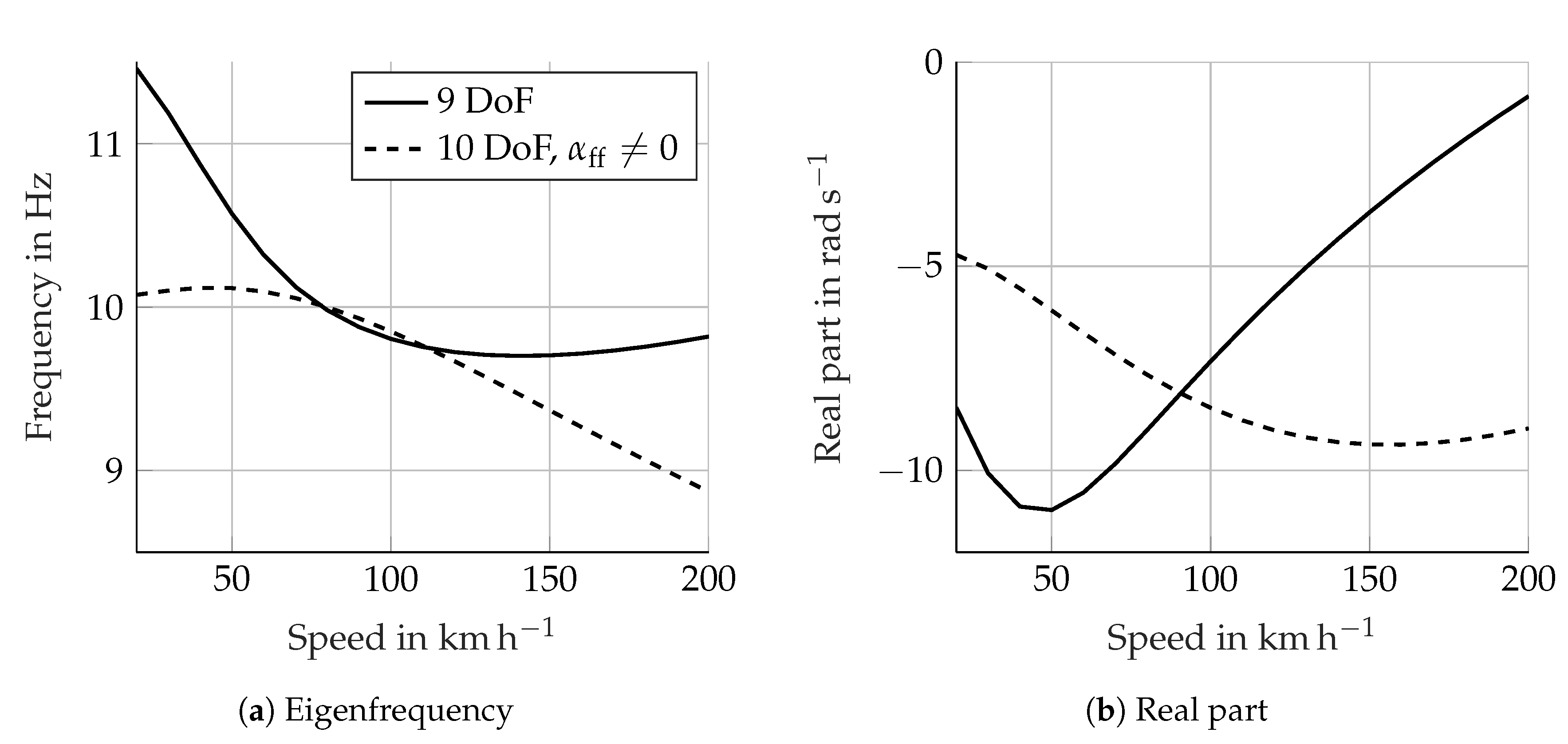
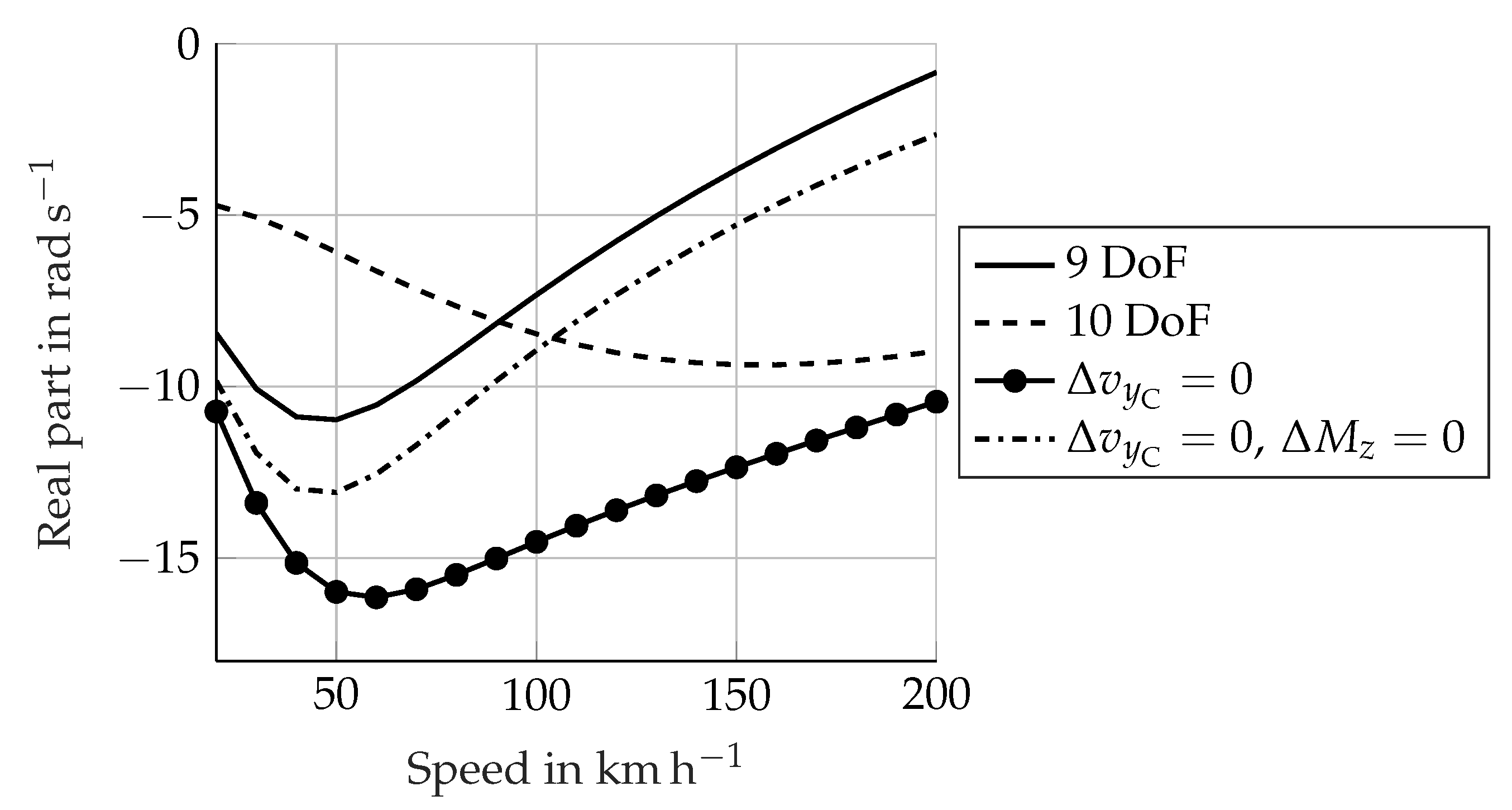
Section 2 describes how the front fork lateral flexibility (bending-compliance about the x axis) strongly influences the stability of wobble. This difference is shown in Figure 4. In order to isolate the influence of the fork compliance, the curve relative to the rigid fork was obtained with a 9-DoF model, wherein the DoF used to represent the motorcycle’s stiffnesses, as described in Section 3.1, have been eliminated. Moreover, the rider’s DoF are not present. In the curve relative to the flexible fork, only the DoF ${\alpha }_{\mathrm{ff}}$ has been added, so that the DoF are 10 in total. With the parameter set used in the present work and in the speed range considered, the wobble mode remains well damped. This is due to the relatively high value of the steering damper. In the following part of this section, the reason for such a drastic behaviour change between rigid and flexible fork is addressed. In particular, a possible cause is presented which partially differs from the explanation provided by Cossalter [2] (p. 280) and Spierings [6].

A key concept described in Section 2 is the correlation between tyre properties and wobble. In particular, a tyre model with cornering stiffness is necessary to reproduce wobble [3,16,17,20]. Therefore, the tyre and specifically the lateral force due to the slip angle is a fundamental factor when considering wobble stability. However, what is the reason for the behaviour inversion in Figure 4 and how can it be attributed to the tyre response? Equation (2) shows how the slip angle depends on the lateral velocity of the wheel contact point $v_{y_{\mathrm{C}}}$. The fork lateral flexibility allows some lateral motion of the wheel because of the rotation about the revolute joint axis (fork x axis), thereby influencing $v_{y_{\mathrm{C}}}$.

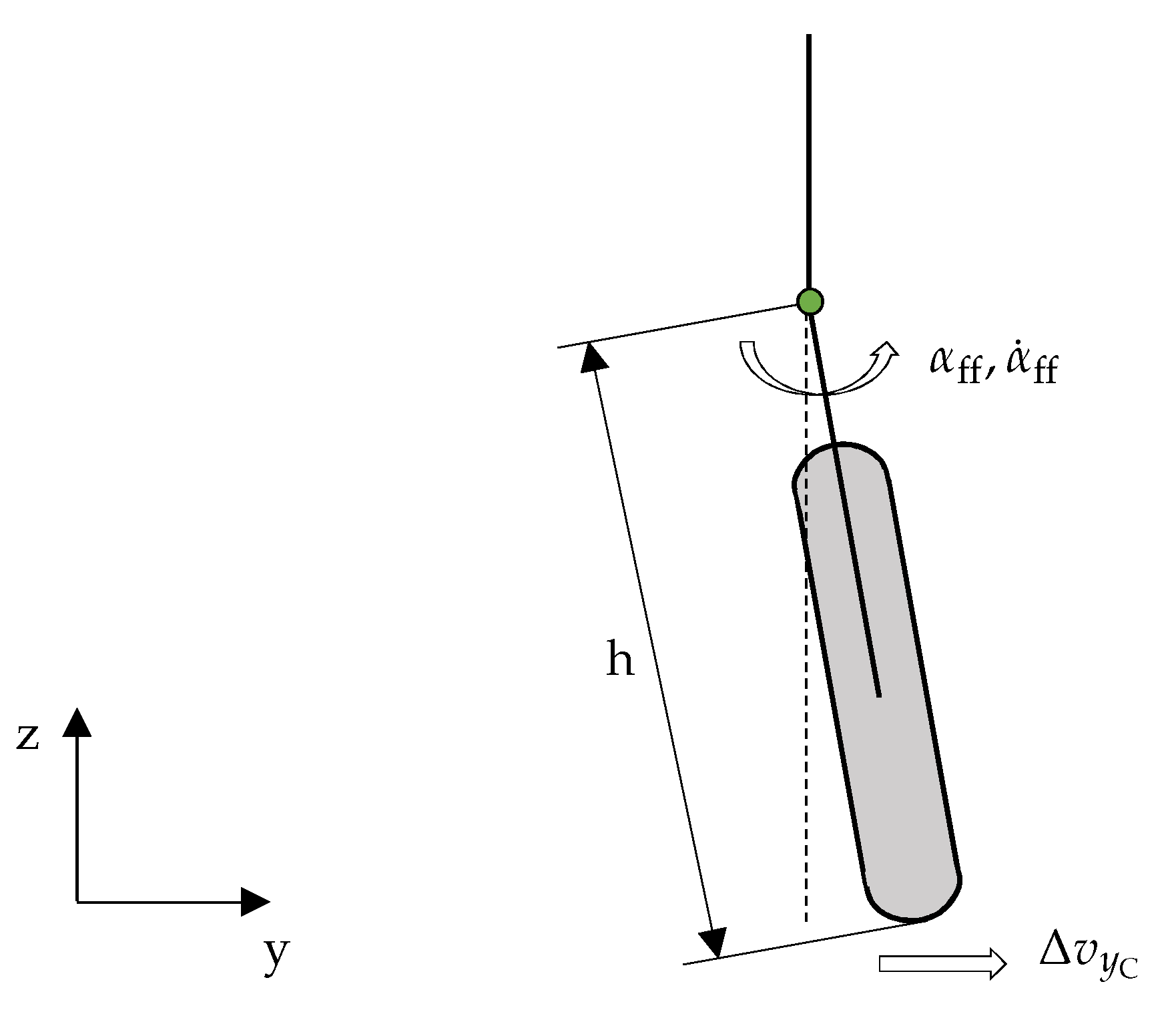
This concept is shown schematically in Figure 5. The variation of $v_{y_{\mathrm{C}}}$ due to the fork lateral flexibility can be expressed as:

$$\Delta v_{y_{\mathrm{C}}}=h{\dot{\alpha }}_{\mathrm{ff}}.$$

(8)

To prove the effect of $\Delta v_{y_{\mathrm{C}}}$, it is compensated by subtracting its value from $v_{y_{\mathrm{C}}}$ in Equation (2). Figure 6 shows the corresponding eigenvalue analysis with the dots-marked curve. The compensation of $\Delta v_{y_{\mathrm{C}}}$ remarkably stabilises wobble. Moreover the curve shows the same behaviour for the 9-DoF model. At this point a conclusion can be drawn: the fork lateral flexibility influences the wobble stability through its effect on the lateral velocity $v_{y_{\mathrm{C}}}$ of the contact point.

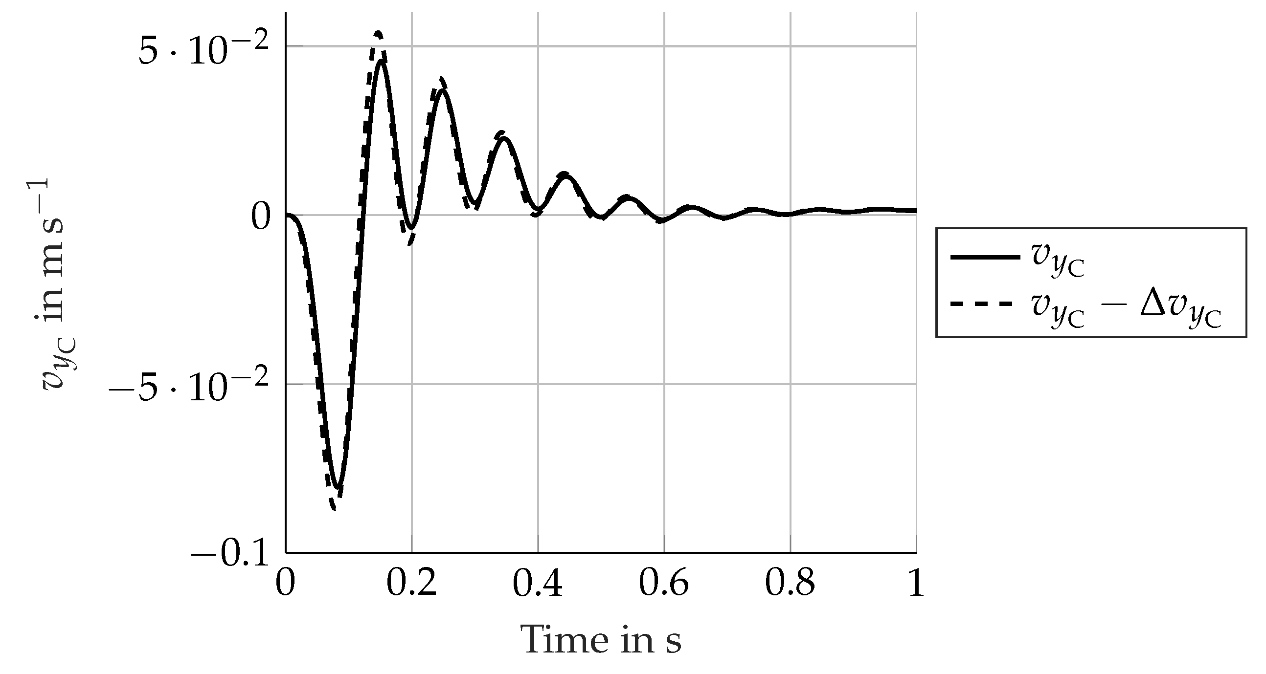
In a subsequent step, it is of particular interest to observe whether $\Delta v_{y_{\mathrm{C}}}$ increases or reduces the value of $v_{y_{\mathrm{C}}}$. Figure 7 shows a time simulation at 50 $\mathrm{k}$$\mathrm{m}$ $\mathrm{h}$⁻¹ with a steer torque impulse as excitation. The full line represents $v_{y_{\mathrm{C}}}$ obtained from Equation (5); the dashed line was obtained with $v_{y_{\mathrm{C}}}-\Delta v_{y_{\mathrm{C}}}$, whereby $\Delta v_{y_{\mathrm{C}}}$ was derived from Equation (8). The subtraction of $\Delta v_{y_{\mathrm{C}}}$ increases the value of $v_{y_{\mathrm{C}}}$: $\Delta v_{y_{\mathrm{C}}}$, which is normally included in $v_{y_{\mathrm{C}}}$, thereby reduces the amplitude of $v_{y_{\mathrm{C}}}$. The tyre-lateral force is proportional to the slip angle, which is proportional to $v_{y_{\mathrm{C}}}$ (Equation (2)). This force tends to oppose the wheel motion due to the wobble oscillation. Therefore, the fork flexibility introduces a $\Delta v_{y_{\mathrm{C}}}$, which reduces the tyre-lateral force. This explains why the curve with $\Delta v_{y_{\mathrm{C}}}=0$ in Figure 6 is significantly more stable than the 10-DoF case with $\Delta v_{y_{\mathrm{C}}}\ne 0$.

Even if the curve with compensated $\Delta v_{y_{\mathrm{C}}}$ in Figure 6 assumes the same qualitative behaviour as the 9-DoF model, the damping values are still significantly different. In order to get a curve similar to that of the 9-DoF model, the gyroscopic moment introduced by fork bending must be compensated. The moment acts about the steering axis and can be calculated with Equation (9) (this formula differs from the complete Euler equations (compare to Equation (10)), whose left-hand side defines the whole gyroscopic effects. Equation (9) is used here because its simple structure allows one to compensate the gyroscopic effects about the steering axis as external moments in the used multibody simulation software), as shown by Cossalter [5]. This formula is also well-known in the literature, as it is present in the book on vehicle dynamics by Mitschke [44]. The symbol $\Delta$ in Equation (9) indicates that the formula only refers to the gyroscopic moment due to the fork lateral flexibility.

$$\Delta M_z={\dot{\alpha }}_{\mathrm{ff}}{\omega }_{y_{\mathrm{fw}}}{I}_{y{y}_{\mathrm{fw}}},$$

(9)

where ${\omega }_{y_{\mathrm{fw}}}$ is the front wheel rotation speed and $I_{y{y}_{\mathrm{fw}}}$ is its polar moment of inertia. The dash-dotted curve in Figure 6 shows the effect of compensating $\Delta M_z$. As expected, the damping curve gets very close to the 9-DoF model. The remaining offset can be attributed to other secondary phenomena, which have not yet been completely identified.

In summary, the influence of the fork bending compliance on wobble can be explained by considering two main phenomena:

• Gyroscopic moment;
• Variation of the lateral speed of the wheel contact point.

Both of them originate through the rotation ${\alpha }_{\mathrm{ff}}$ and its time derivatives.

When observing the curve of the 10-DoF case in Figure 6, it is evident that it is less stable than the 9-DoF case only up to about 80 $\mathrm{k}$$\mathrm{m}$ $\mathrm{h}$⁻¹. Above this speed, the higher stability of the 10-DoF model compared to the 9-DoF model can be justified with the same consideration made by Cossalter [5]: the gyroscopic moment $\Delta M_z$ about the steering axis stabilises the wobble with increasing speed.

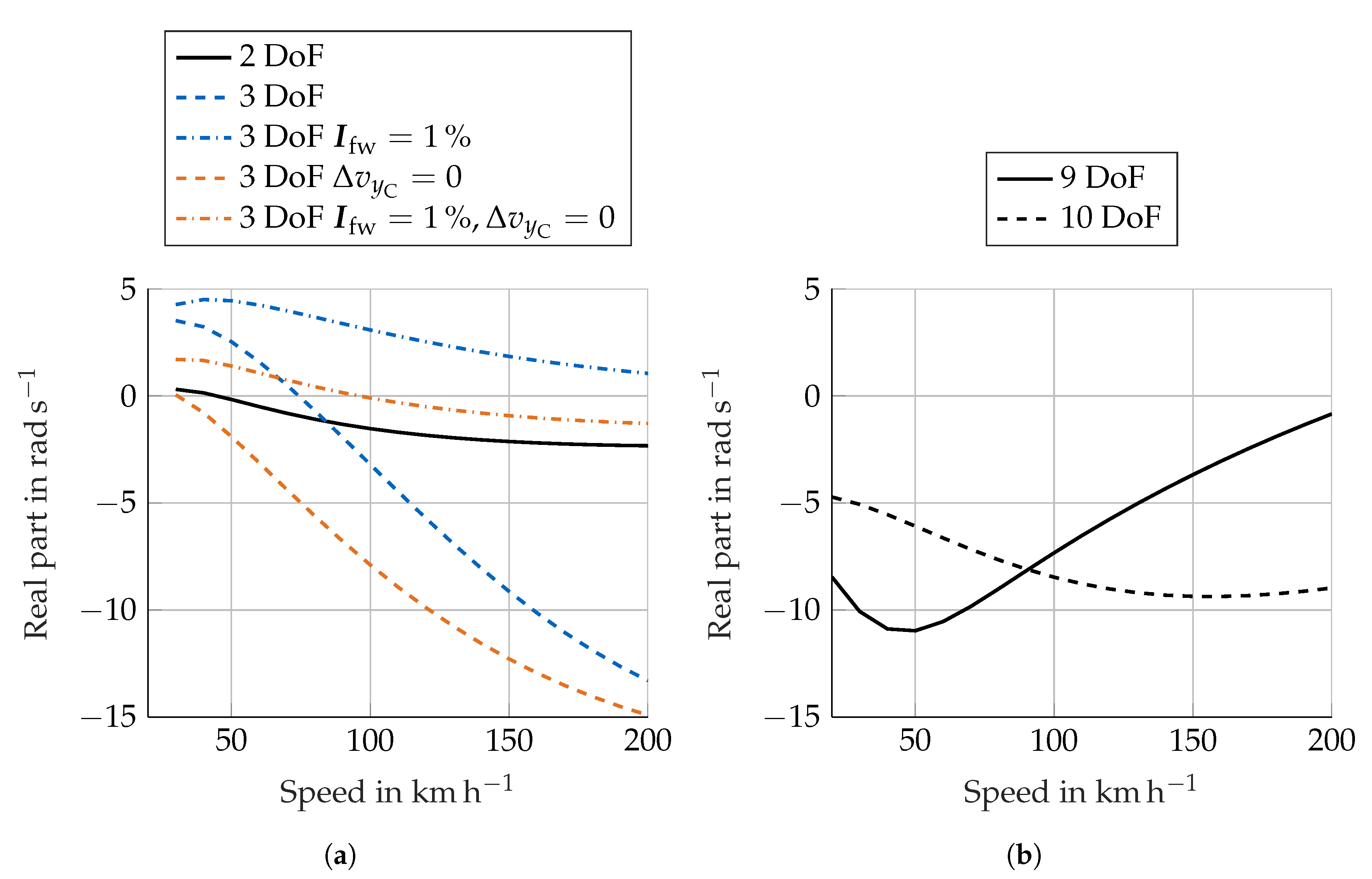
At this point another question may be raised: Which phenomenon is responsible for the decreasing wobble damping shown by the 9-DoF model and the model with compensated $\Delta v_{y_{\mathrm{C}}}$ compared to the 10-DoF one? To answer this question, a model containing only the front fork and front wheel has been used. With this model two cases are studied: two DoF characterised by the rigid fork and three DoF with a flexible fork; the first model correlates with the 9-DoF model, and the second with the 10-DoF model.

Figure 8a shows the damping curves for these two models. Different variations were made: the wheel inertia tensor ${\mathit{I}}_{\mathrm{fw}}$ was set to 1% of the original value (to eliminate the gyroscopic moments) and $\Delta v_{y_{\mathrm{C}}}$ has been compensated as in Figure 6. Some important conclusions can be drawn:

• The 2-DoF model did not show a decrease in damping with increasing speed, as did the 9-DoF model.
• The damping of the 3-DoF model grew more rapidly than the one of the 10-DoF model.
• The case ${\mathit{I}}_{\mathrm{fw}}=1\%,\Delta v_{y_{\mathrm{C}}}=0$ is very close to the curve of the 2-DoF model, as was expected by to theoretical observations. In fact, the 2-DoF model had no gyroscopic moments about the steering axis, as no rotation about the fork x axis was present. In Figure 6 the curve with $\Delta v_{y_{\mathrm{C}}}=0$ shows a remarkable offset compared to the 9-DoF curve because of the gyroscopic moments. With ${\mathit{I}}_{\mathrm{fw}}$ set to $1\%$ they almost vanish, resulting in a smaller offset.

The difference in behaviour between the 2 and 9-DoF models can be justified by the additional roll motion of the 9-DoF case. This motion produces additional gyroscopic moments which apparently destabilise the wobble with increasing speed. These moments are also clearly present in the 10-DoF model. However, in this case they are compensated by the gyroscopic moment produced by the fork flexibility. The opposition of these two effects is underlined by the saturation shown in the 10-DoF model at about 150 $\mathrm{k}$$\mathrm{m}$ $\mathrm{h}$⁻¹, which is not present in the 3-DoF model.

In summary, the wobble damping behaviour of a real motorcycle is determined by three principal mechanisms. The front fork flexibility produces a lateral movement of the front wheel, which can be represented with a rotation ${\alpha }_{\mathrm{ff}}$. This reduces the tyre-lateral force and thus decreases the wobble damping at low speed compared to a rigid fork. When the speed increases, the gyroscopic moment caused by the rotation ${\alpha }_{\mathrm{ff}}$ increases in magnitude and stabilises the wobble, thereby making the 10 DoF model more stable than the 9-DoF model. The third mechanism is related to the gyroscopic moments caused by the motorcycle’s roll motion. They destabilise the wobble with increasing speed, thereby explaining why the wobble damping in the 9-DoF model decreases with increasing speed. This does not happen in the 10-DoF model because the stabilising gyroscopic moment caused by ${\alpha }_{\mathrm{ff}}$ outweighs the destabilising effect.

4.2. Weave

The weave mode was already captured in its essence by the very first motorcycle model by Whipple [13] (p. 195). Moreover, there is no evidence of parameters which produce a behaviour inversion of the damping curve, as can be observed for the wobble mode. This already suggests that the weave mode reproduces in some way the "basic" motorcycle behaviour. This idea was also proposed by Schröter [45] (p. 28), who describes the weave mode as a degenerated dynamic stabilisation process involving steering, roll and yaw oscillations. This can be shown with a simple time simulation where the upright riding motorcycle is excited with a lateral force impulse applied to the frame. Assuming that the wobble is well damped, the motorcycle reacts to this excitation with a weave oscillation, which may diverge or stabilise depending on the motorcycle’s speed and parameters.

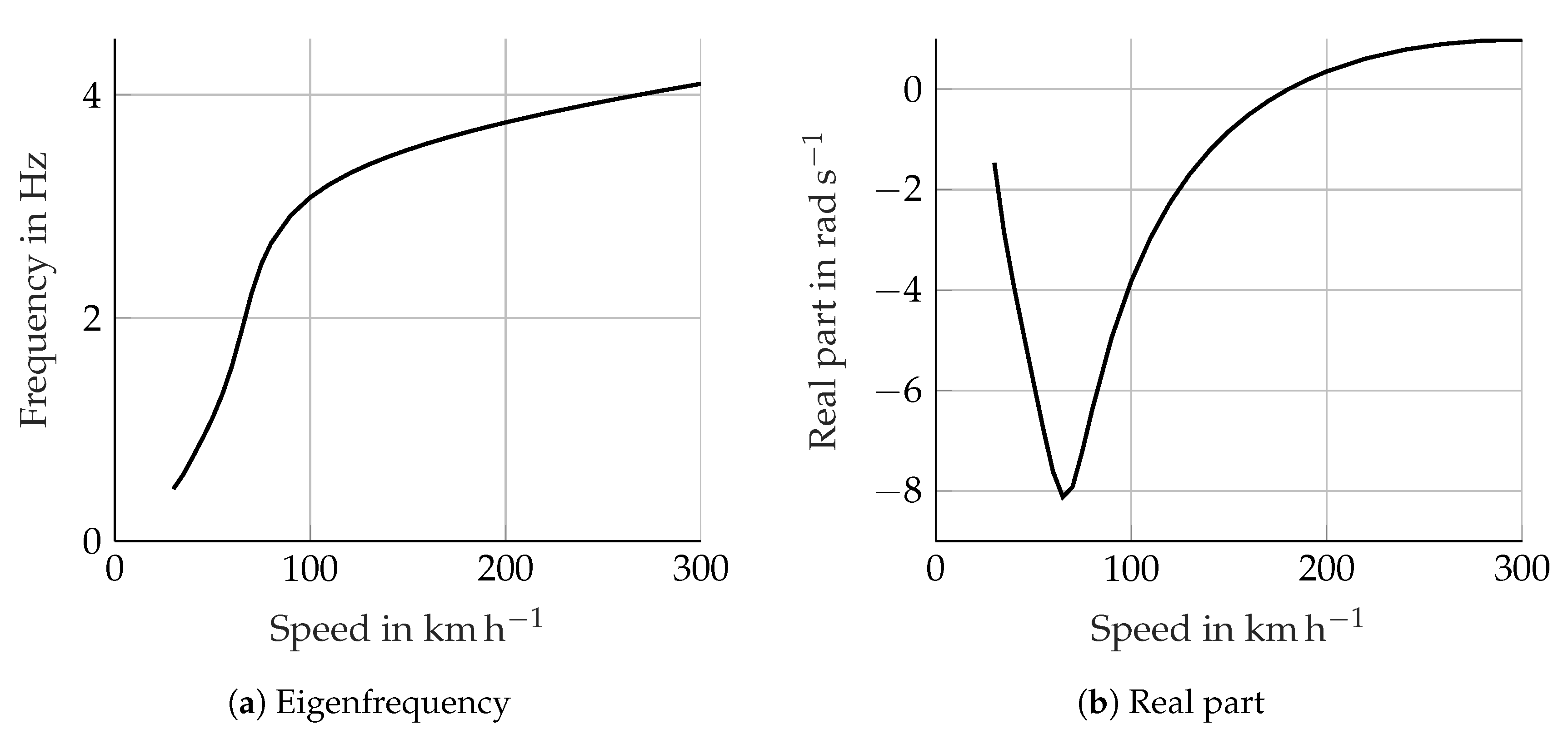
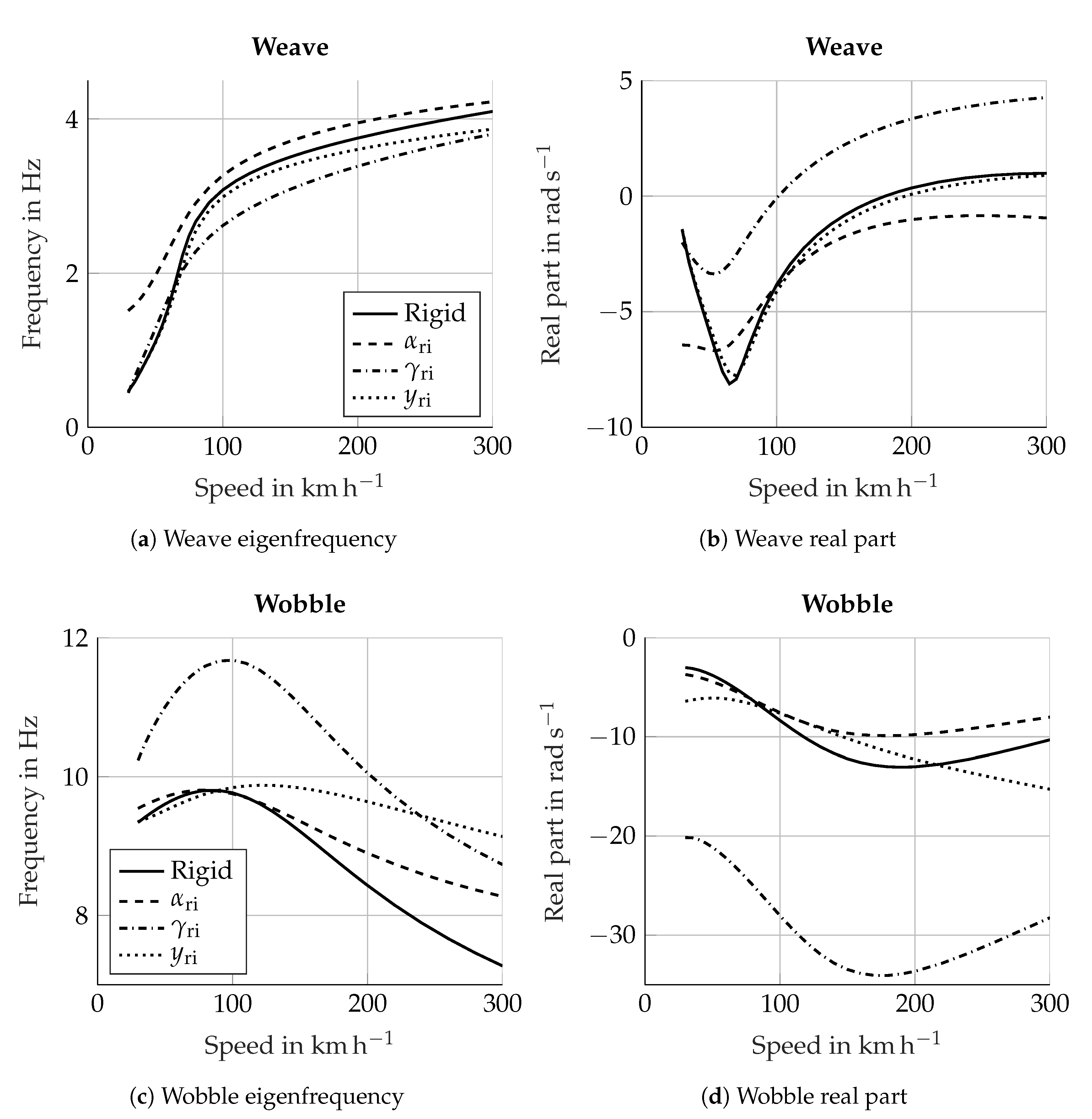
Figure 9 shows the frequency and damping of the weave mode as a function of the speed. The effect of the rider is analysed in Section 4.3, so this figure refers to the case with a rigid rider; the other DoF are all present. In order to represent the saturation shown by the damping curve at high speed, the speed range differs from the one in Figure 4. The behaviour of the weave damping shows some interesting characteristics: below 70 $\mathrm{k}$$\mathrm{m}$ $\mathrm{h}$⁻¹ weave is stabilised with increasing speed; above it is destabilised. However, above 220 $\mathrm{k}$$\mathrm{m}$ $\mathrm{h}$⁻¹ the weave damping shows a plateau. This particular behaviour suggests that the weave mode changes with speed. Moreover, the speed dependency could be explained by a certain influence of the gyroscopic effects, which are also speed dependent. The gyroscopic effects are obtained with the whole left-hand side of the Euler equations, which is shown in Equation (10) for the front wheel.

$${\mathit{I}}_{\mathrm{fw}}{\dot{\mathit{\omega }}}_{\mathrm{fw}}+{\mathit{\omega }}_{\mathrm{fw}}\times \left({\mathit{I}}_{\mathrm{fw}}{\mathit{\omega }}_{\mathrm{fw}}\right)={\mathit{M}}_{\mathrm{ext}},$$

(10)

where ${\mathit{\omega }}_{\mathrm{fw}}$ is the rotational velocity vector of the front wheel and ${\mathit{I}}_{\mathrm{fw}}$ is the front wheel inertia tensor.

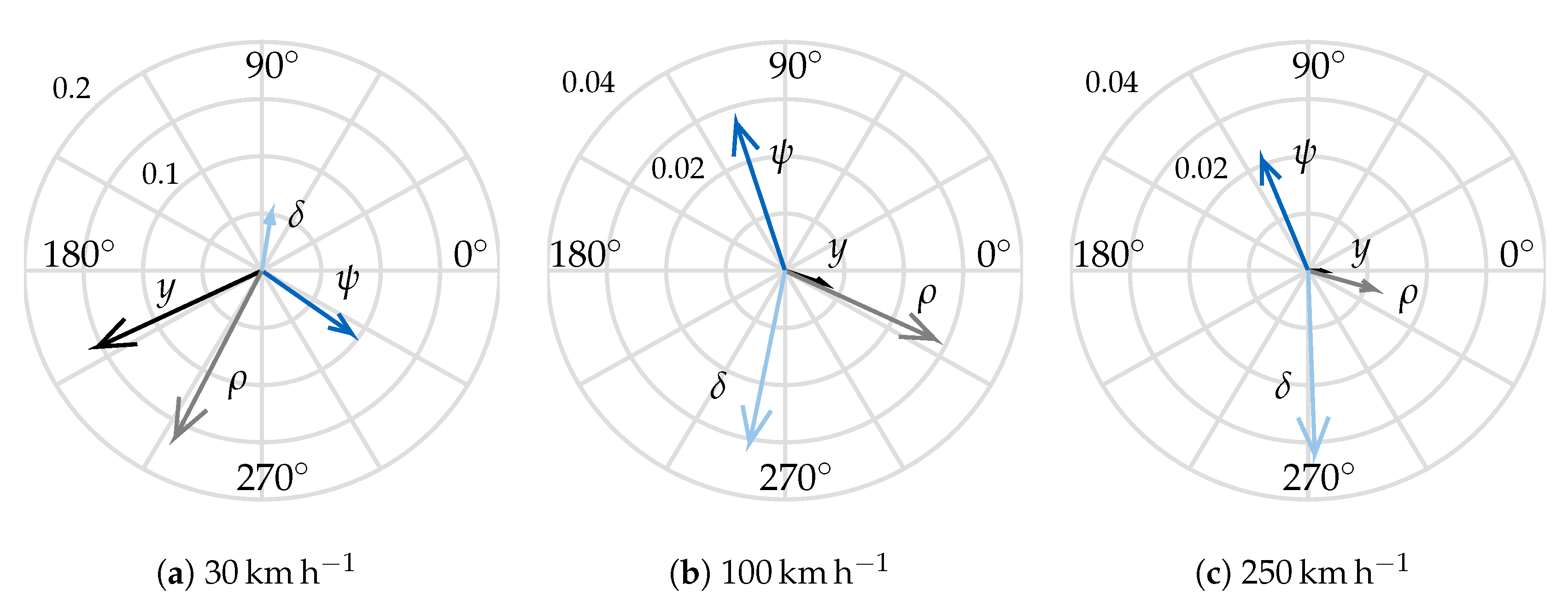
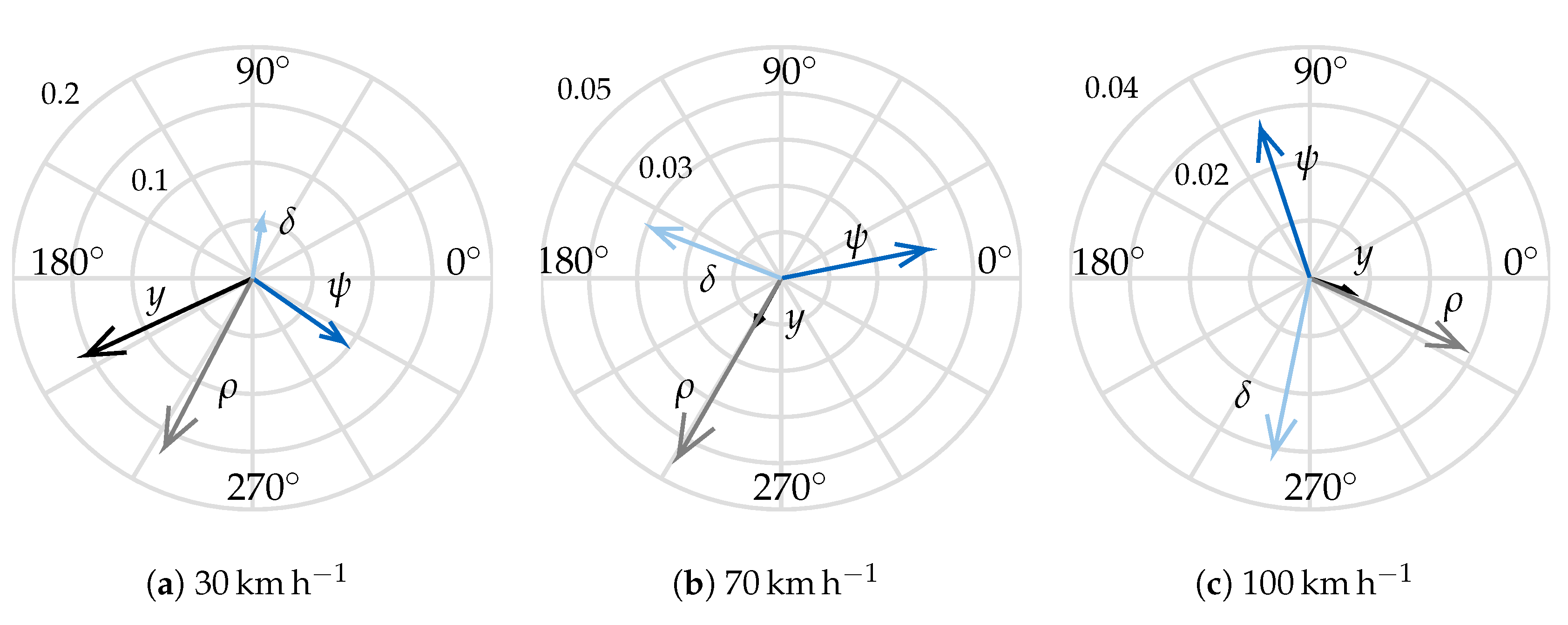
Figure 10 further illustrates this concept. In this figure, the weave eigenvector is shown with the so-called compass plot. The arrows are named phasors and represent how the motorcycle’s DoF are involved in the weave oscillation. An arrow’s length is the magnitude of the motion of the related DoF. In order to maintain the information about the absolute amplitude of the phasors, no normalisation is present. The phasor’s angle shows the phase. In the following paragraphs the relative angle between the phasors is called relative phase.

At low speed, (Figure 10a) the roll ($\rho$) and lateral displacement (y) show big amplitudes. The latter is due to the small gyroscopic effects, so that if weave is excited (for example, with a lateral impulse), the motorcycle describes a “slalom” at low frequency (see Figure 9) involving a significant lateral displacement. This can be described as a low-frequency “self-stabilising” motion, which the literature already considers as weave.

As the speed increases (Figure 10b), the relative phase between the motions significantly changes, whereby the lateral displacement is no longer important. The other DoF show a similar amplitude. Finally, when the speed increases further (Figure 10c), the relative phase does not change remarkably. The most important observation, however, is the reduction of the roll ($\rho$) amplitude with increasing speed, which can be seen when comparing the related phasor in Figure 10b,c. This can also be observed in the time simulation. If the motorcycle is excited by a lateral impulse at high speed, the resulting weave oscillation does not show a significant roll motion, while the front wheel and the frame rotate around the steering and vertical axis almost in opposition of phase, as shown by the vectors $\delta ,\psi$ in Figure 10c. The reduction in roll motion with increasing speed is also shown by a free rolling wheel. This phenomenon can be explained considering the gyroscopic effects which increase with speed, thereby preventing the wheel (or the motorcycle) capsizing.

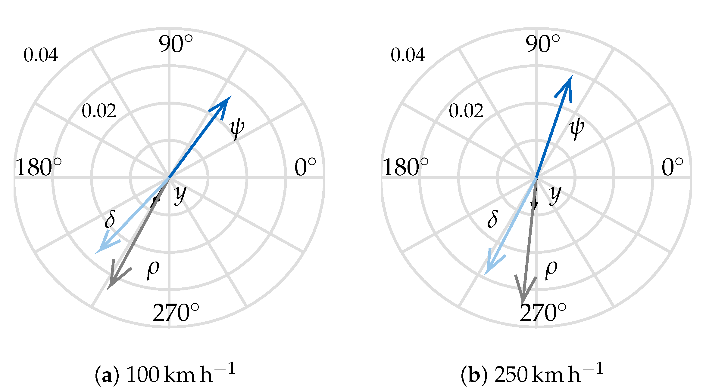
Which are the possible causes of the peculiar damping behaviour shown in Figure 9b? Some useful knowledge can be derived by an eigenvalue analysis with reduced wheel inertia. The correlation to Figure 10 is shown in Figure 11, for which the total wheel inertia tensors ${\mathit{I}}_{\mathrm{fw}},{\mathit{I}}_{\mathrm{rw}}$ was set to 10% of the original tensors. The first consideration resulting from the comparison is that in Figure 11 the relative phase between the phasors no longer changes with speed, as it happens in Figure 10. The plot at 30 $\mathrm{k}$$\mathrm{m}$ $\mathrm{h}$⁻¹ is not present, as the weave mode is no longer available at this speed. It is important to point out that, because of this massive inertia reduction, the gyroscopic effects almost disappear. Two main observations can be made:

• The missing weave mode at low speed can be attributed to the (almost) missing gyroscopic effects. The time simulation at 30 $\mathrm{k}$$\mathrm{m}$ $\mathrm{h}$⁻¹ with a lateral force impulse shows that the motorcycle does not react to the excitation with a weave oscillation, but it capsizes. With the original inertia values the gyroscopic effects are present, despite the low speed. They prevent the motorcycle from capsizing immediately after the excitation and producing the low-frequency “self-stabilising” motion.
• The gyroscopic effects are also the main cause for the change in the weave eigenvector shown in Figure 10. In fact, when they are very small, as in Figure 11, the relative phase between the eigenvector components is no longer speed dependent.

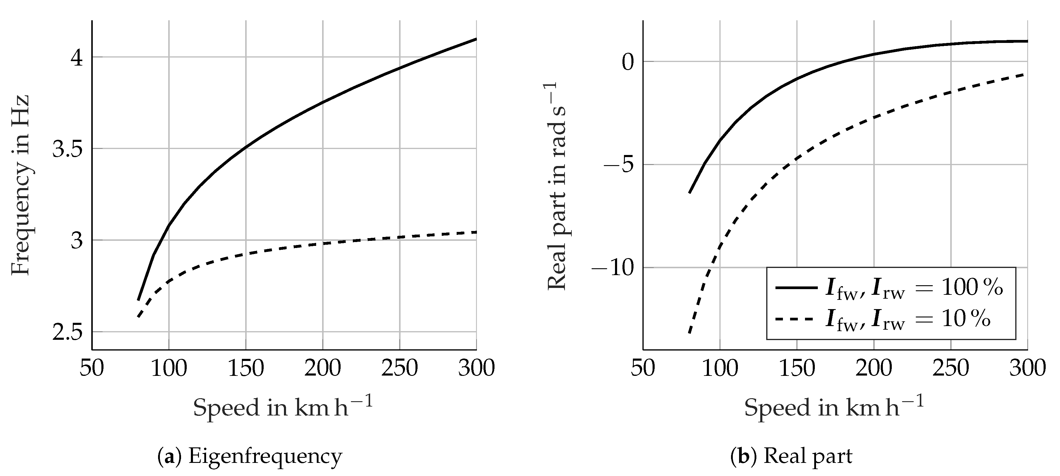
The correlation with Figure 9 is shown in Figure 12. The speed range starts now from 80 $\mathrm{k}$$\mathrm{m}$ $\mathrm{h}$⁻¹, as for the following reasoning only this range is necessary. Moreover, the weave with reduced wheel inertia is not present up to about 50 $\mathrm{k}$$\mathrm{m}$ $\mathrm{h}$⁻¹ and in the range 50 $-80$ $\mathrm{k}$$\mathrm{m}$ $\mathrm{h}$⁻¹ it is extremely well damped (real part > 25 $\mathrm{rad}$ $\mathrm{s}$⁻¹). Similarly to the full inertia case, the damping continues to decrease with increasing speed in the small inertia case shown in Figure 12b. As the gyroscopic effects are almost missing, the reason for this behaviour can be determined by investigating in the tyre response. The tyre-lateral force is proportional to the slip angle which is in turn proportional to the ratio between $v_{y_{\mathrm{C}}}$ and $v_{x_{\mathrm{C}}}$ (Equation (2)). The authors verified that $v_{y_{\mathrm{C}}}$ mainly depends on the kinematic steering angle (see [2] for its definition), which is proportional to the steering angle. Figure 11 shows that above a certain speed (100 $\mathrm{k}$$\mathrm{m}$ $\mathrm{h}$⁻¹) the amplitude of steering motion in the weave eigenvector remains fairly constant. The numerator of ${\alpha }_{\mathrm{ss}}$ in Equation (2) is therefore almost constant with speed. The denominator of ${\alpha }_{\mathrm{ss}}$ is given by $v_{x_{\mathrm{C}}}$, which clearly increases with speed. As a result, ${\alpha }_{\mathrm{ss}}$ decreases with increasing speed and so does the tyre-lateral force. The tyre-lateral forces tend to bring the motorcycle back to the equilibrium position, thereby stabilising the weave. The decreasing tyre force is therefore responsible for the decreasing weave damping and the hyperbolic behaviour of the dashed curve in Figure 12b.

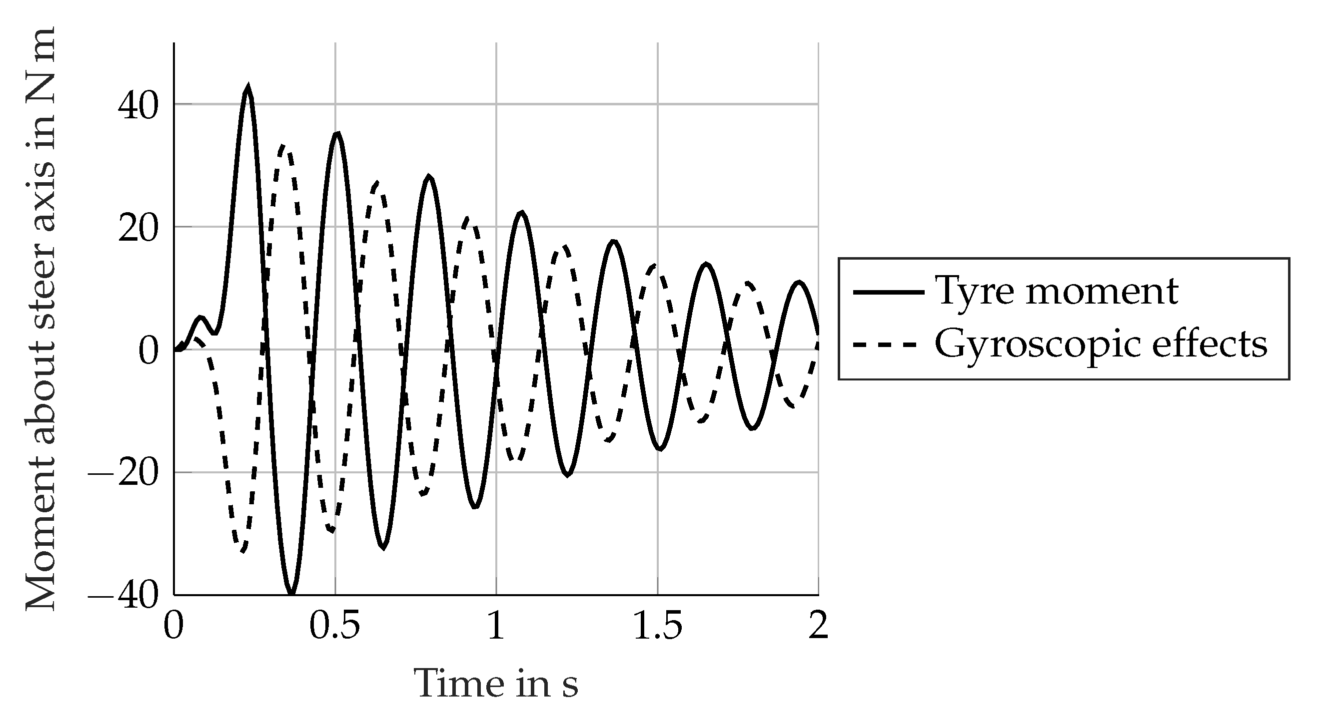
Considering again the curve with the original wheel inertia in Figure 12, the first observation is the smaller weave damping. This can be explained by taking into account the additional impact of the gyroscopic effects. The gyroscopic effects of the front wheel about the steering axis are in counterphase with respect to the tyre moments, as Figure 13 shows, therefore they work against them. For this reason, the weave damping is lower compared to the reduced inertia case. The gyroscopic effects also justify the slower damping decrease in the case with original wheel inertia (see Figure 12). In fact, due to the progressively changing eigenvector (Figure 10), i.e., the decreasing roll motion amplitude, the gyroscopic effects increase underproportionally with the speed. For example, in a time simulation with lateral force excitation, the first peak of the front wheel gyroscopic effects about the z axis increase from 100 to 150 $\mathrm{k}$$\mathrm{m}$ $\mathrm{h}$⁻¹ by 37.5%, while they only increase by 14.5% from 250 to 300 $\mathrm{k}$$\mathrm{m}$ $\mathrm{h}$⁻¹. As a consequence, they also underproportionally reduce the tyre forces with increasing speed. This, combined with the decreasing tyre forces, leads to the mentioned saturation above 220 $\mathrm{k}$$\mathrm{m}$ $\mathrm{h}$⁻¹, which is not present in the reduced inertia case.

The last characteristic to be observed is the increase in damping shown below 80 $\mathrm{k}$$\mathrm{m}$ $\mathrm{h}$⁻¹ in Figure 9b. The authors’ belief is that in this lower speed range the weave mode can still be seen as the already mentioned low-speed “self-stabilising” motion. When increasing the speed, this motion progressively changes to the “real” weave, thereby producing the observed increase in damping. Figure 14 illustrates this fact. Following the three compass plots with increasing speed, one can see that the phase and amplitude of the phasors progressively change; i.e., the weave changes from the “self-stabilising” motion to the classical weave. In fact, above 100 $\mathrm{k}$$\mathrm{m}$ $\mathrm{h}$⁻¹ the relative angle between the phasors no longer changes significantly, as the comparison of Figure 10b,c shows.

4.3. Rider Influence

As explained in Section 3.3, the literature offers different examples of rider modelling. These references often analyse the influences of the rider on weave and wobble stability. For example, reference [42] investigates the effect of the rider yaw combined with the connection to the handlebar. Reference [7] proposes the eigenvalue analysis with the 3-DoF rider also used in the present work. In order to obtain a better overview of the single influences, this section aims to briefly summarise the essential differences between the three different DoF models used for rider modelling. This is shown in Figure 15. The effect of the single DoF can be summarised as follows:

• The rider lean ${\alpha }_{\mathrm{ri}}$ stabilises the weave and destabilises the wobble at high speed. The increased stability of weave is a reasonable result because during the weave oscillation the rider lean is almost in counterphase to the motorcycle’s roll [41], thereby damping out this motion.
• The rider yaw ${\gamma }_{\mathrm{ri}}$ combined with the connection to the handlebar destabilises the weave, massively stabilises the wobble and also increases its eigenfrequency. This is in accordance with [42] and is a reasonable result, as the connection acts in a similar way to a steering damper, which also stabilises the wobble while destabilising the weave.
• The rider’s hip lateral motion $y_{\mathrm{ri}}$ hardly affects the eigenmodes, as also reported by [31]. The only remarkable influence is the increase in the wobble frequency at high speed.

Figure 16 shows the effect of the whole rider model, containing the three DoF ${\alpha }_{\mathrm{ri}},y_{\mathrm{ri}},{\gamma }_{\mathrm{ri}}$. In the weave the effect of ${\alpha }_{\mathrm{ri}}$ overcomes the others, thereby causing the already mentioned stabilisation at high speed. When concerning wobble, the effect of ${\gamma }_{\mathrm{ri}}$ and the connection with the handlebar are dominant, leading to an increase in both frequency and damping.

5. Conclusions and Outlook

The present work further analysed the physical phenomena behind the wobble and weave eigenmodes. In particular, the effect of the front fork bending compliance has been discussed and a possible justification for the well-known weave damping behaviour with increasing speed is provided. Finally, the effect of the single rider’s DoF on the weave and wobble mode has been shown.

The first aspect has been addressed before by Cossalter [5] and Spierings [6]. They noticed that the modelling of the fork bending compliance allows very similar results to the real driving experience to be obtained: the wobble mode is unstable at low speed and stabilises with increasing speed. Without this parameter, the simulation results are not realistic. Cossalter [5] justifies this behaviour considering the superposition of two effects, both caused by the fork bending compliance: this compliance alone is destabilising but it also produces a gyroscopic moment about the steering axis that stabilises the wobble. The first effect dominates at low speeds, while the second prevails at high speed. The present work provides an additional perspective for explaining the effect of the fork bending compliance, though maintaining the validity of the previous results [5]. The additional insight is given by the tyre behaviour. It was demonstrated that the lateral motion of the wheel contact point caused by the fork bending compliance reduces the lateral component of the contact point velocity $v_{y_{\mathrm{C}}}$. The tyre-lateral force is proportional to this velocity component through the slip angle. Reducing $v_{y_{\mathrm{C}}}$ also reduces the tyre force. This causes a reduction in the wobble damping at below 80 $\mathrm{k}$$\mathrm{m}$ $\mathrm{h}$⁻¹. At higher speeds, the effect of the gyroscopic moments introduced by the fork flexibility leads to increasing wobble damping with increasing speed, as explained by Cossalter [5].

The weave damping behaviour is well-known and involves a progressive stabilisation up to about 80 $\mathrm{k}$$\mathrm{m}$ $\mathrm{h}$⁻¹ (with the present parameters), then the damping decreases with increasing speed until it reaches a saturation above 220 $\mathrm{k}$$\mathrm{m}$ $\mathrm{h}$⁻¹. This peculiar behaviour can now be explained. The weave eigenvector changes with speed. In the lower speed range this corresponds to a change from a low frequency self-stabilising motion involving a lot of frame lateral displacement to a weave oscillation where the lateral motion is no longer significant. The eigenvector change is supposed to be the main cause of the damping increase below 80 $\mathrm{k}$$\mathrm{m}$ $\mathrm{h}$⁻¹. Above this lower speed range, the weave eigenvector does not change in the relative phase between phasors, but the roll component becomes progressively smaller. This influences the gyroscopic effects, which underproportionally increase with speed, thereby causing the plateau above 220 $\mathrm{k}$$\mathrm{m}$ $\mathrm{h}$⁻¹.

The multibody model used in this work was provided with a functionality to select the different DoF. This gives the chance to investigate the separated influence of the single DoF used in the rider model. In particular, the rider lean stabilises the weave and slightly destabilises the wobble; the rider yaw plus the connection with the handlebar destabilises the weave and remarkably stabilises the wobble. The whole 3-DoF rider model produces the same effect of the rider lean as regards weave and the same effect of rider yaw as regards wobble.

The contributions of the present paper to general motorcycle dynamics knowledge can be summarised as follows. A review of the literature on motorcycle dynamics and stability behaviour; this knowledge has been interpreted in order to derive some minimal prerequisites to the motorcycle model, with the aim of conducting a stability analysis. After that, the effect of the tyre response on the wobble damping was analysed, thereby leading to considerations that fuse together with and partially complete the theory exposed by Cossalter [5] and Spierings [6]. Moreover, a possible justification for the well-known weave damping behaviour was given, which was not found in the literature. Finally, the influence of the rider model on stability, which was already studied in previous works, has been summarised, thereby facilitating the interpretation of the effect of the single rider’s DoF.

Further development of the present paper could involve the inclusion of a “flexible body” to faithfully reproduce the different frame flexibilities without using lumped stiffnesses.

References

1. Sharp, R.S. Stability, Control and Steering Responses of Motorcycles. Veh. Syst. Dyn. 2001, 35, 291–318. [Google Scholar] [CrossRef]
2. Cossalter, V. Motorcycle Dynamics, 2nd ed.; Lulu Press: Morrisville, NC, USA, 2006. [Google Scholar]
3. Sharp, R.S. The stability and control of motorcycles. J. Mech. Eng. Sci. 1971, 13, 316–329. [Google Scholar] [CrossRef] [Green Version]
4. Koch, H. Zusammenhänge und Einflüsse von Lebensalter, Fahrerfahrung und Motorleistung auf die Unfallverwicklung von Motorradfahranfängern; VDI-Berichte: Düsseldorf, Germany, 1987. [Google Scholar]
5. Cossalter, V.; Lot, R.; Massaro, M. The influence of frame compliance and rider mobility on the scooter stability. Veh. Syst. Dyn. 2007, 45, 313–326. [Google Scholar] [CrossRef]
6. Splerings, P.T.J. The Effects of Lateral Front Fork Flexibility on the Vibrational Modes of Straight-Running Single-Track Vehicles. Veh. Syst. Dyn. 1981, 10, 21–35. [Google Scholar] [CrossRef]
7. Cossalter, V.; Lot, R.; Massaro, M. An advanced multibody code for handling and stability analysis of motorcycles. Meccanica 2011, 46, 943–958. [Google Scholar] [CrossRef]
8. Koenen, C.; Pacejka, H.B. The Influence of Frame Elasticity and Simple Rider Body Dynamics on Free Vibrations of Motorcycles in Curves. Veh. Syst. Dyn. 1981, 10, 70–73. [Google Scholar] [CrossRef]
9. Cossalter, V.; Doria, A.; Mitolo, L. Inertial and Modal Properties of Racing Motorcycles; SAE Technical Papers; SAE International: Warrendale, PA, USA, 2002. [Google Scholar]
10. Wisselmann, D. Motorrad-Fahrdynamik-Simulation. Modellbildung, Validierung und Anwendung. Ph.D. Thesis, VDI-Berichte, Dachau, Germany, 1992. [Google Scholar]
11. Schindler, T.; Förg, M.; Friedrich, M.; Schneider, M.; Esefeld, B.; Huber, R.; Zandler, R.; Ulbrich, H. Analysing Dynamical Phenomenons: Introduction to MBSim. In Proceedings of the 1st Joint International Conference on Multibody System Dynamics, Lappeenranta, Finland, 25–27 May 2010. [Google Scholar]
12. Sharp, R.S.; Evangelou, S.A.; Limebeer, D.J.N. Advances in the Modelling of Motorcycle Dynamics. Multibody Syst. Dyn. 2004, 12, 251–283. [Google Scholar] [CrossRef] [Green Version]
13. Limebeer, D.J.N.; Massaro, M. Dynamics and Optimal Control of Road Vehicles; Oxford University Press: Oxford, UK, 2018. [Google Scholar]
14. Cossalter, V.; Doria, A.; Massaro, M.; Taraborrelli, L. Experimental and numerical investigation on the motorcycle front frame flexibility and its effect on stability. Mech. Syst. Signal Process. 2015, 60–61, 452–471. [Google Scholar] [CrossRef]
15. Meirovitch, L. Elements of Vibration Analysis; Mc Grow Hill: New York, NY, USA, 1975. [Google Scholar]
16. Doria, A.; Favaron, V.; Taraborrelli, L.; Roa, S. Parametric analysis of the stability of a bicycle taking into account geometrical, mass and compliance properties. Int. J. Veh. Des. 2017, 75, 91–123. [Google Scholar] [CrossRef]
17. Doria, A.; Roa, S. On the influence of tyre and structural properties on the stability of bicycles. Veh. Syst. Dyn. 2018, 56, 947–966. [Google Scholar] [CrossRef]
18. Klinger, F.; Nusime, J.; Edelmann, J.; Plöchl, M. Wobble of a racing bicycle with a rider hands on and hands off the handlebar. Veh. Syst. Dyn. 2014, 52, 51–68. [Google Scholar] [CrossRef]
19. Sharp, R.S.; Alstead, C.J. The Influence of Structural Flexibilities on the Straight-running Stability of Motorcycles. Veh. Syst. Dyn. 1980, 9, 327–357. [Google Scholar] [CrossRef]
20. Plöchl, M.; Edelmann, J.; Angrosch, B.; Ott, C. On the wobble mode of a bicycle. Veh. Syst. Dyn. 2012, 50, 415–429. [Google Scholar] [CrossRef]
21. Roa, S.; Doria, A.; Muñoz, L. Optimization of the Bicycle Weave and Wobble Modes. Am. Soc. Mech. Eng. 2018, 3. [Google Scholar] [CrossRef]
22. Diermeyer, F.; Eisele, A. Lecture notes of the course Motorradtechnik. 2018; Unpublished manuscript. [Google Scholar]
23. Taraborrelli, L.; Favaron, V.; Doria, A. The effect of swingarm stiffness on motorcycle stability: Experimental measurements and numerical simulations. Int. J. Veh. Syst. Model. Test. 2017, 12, 240. [Google Scholar] [CrossRef]
24. Weir, D.H.; Zeller, J.W. Experimental investigation of the transient behaviour of motorcycles. SAE Trans. 1979, 88, 962–978. [Google Scholar]
25. De Vries, E.; Pacejka, H.B. Motorcycle Tyre Measurements and Models. Veh. Syst. Dyn. 1998, 29, 280–298. [Google Scholar] [CrossRef]
26. Pacejka, H.B.; Besselink, I. Tire and Vehicle Dynamics, 3rd ed.; Butterworth-Heinemann: Oxford, UK, 2012. [Google Scholar]
27. Evangelou, S.A.; Limebeer, D.J.N.; Sharp, R.S.; Smith, M.C. Mechanical steering compensators for high-performance motorcycles. J. Appl. Mech. Trans. 2007, 74, 332–346. [Google Scholar] [CrossRef]
28. Sharp, R.S.; Limebeer, D.J.N. A Motorcycle Model for Stability and Control Analysis. Multibody Syst. Dyn. 2001, 6, 123–142. [Google Scholar] [CrossRef]
29. Cossalter, V.; Lot, R.; Maggio, F. A Multibody Code for Motorcycle Handling and Stability Analysis with Validation and Examples of Application. In SAE International400 Commonwealth Drive; SAE Technical Paper Series; SAE International: Warrendale, PA, USA, 2003. [Google Scholar] [CrossRef]
30. Limebeer, D.J.N.; Sharma, A. Burst Oscillations in the Accelerating Bicycle. J. Appl. Mech. Trans. 2010, 77, 061012. [Google Scholar] [CrossRef]
31. Roe, G.E.; Thorpe, T.E. A solution of the low-speed wheel flutter instability in motorcycles. J. Mech. Eng. Sci. 1976, 18, 57–65. [Google Scholar] [CrossRef]
32. Cossalter, V.; Lot, R.; Maggio, F. The Modal Analysis of a Motorcycle in Straight Running and on a Curve. Meccanica 2004, 39, 1–16. [Google Scholar] [CrossRef]
33. Limebeer, D.J.N.; Sharp, R.S.; Evangelou, S.A. Motorcycle Steering Oscillations due to Road Profiling. J. Appl. Mech. Trans. 2002, 69, 724–739. [Google Scholar] [CrossRef] [Green Version]
34. Sharp, R.S. The Influence of the Suspension System on Motorcycle Weave-mode Oscillations. Veh. Syst. Dyn. 1976, 5, 147–154. [Google Scholar] [CrossRef]
35. Lot, R. A Motorcycle Tire Model for Dynamic Simulations: Theoretical and Experimental Aspects. Meccanica 2004, 39, 207–220. [Google Scholar] [CrossRef]
36. Evangelou, S.A.; Limebeer, D.J.N.; Tomas-Rodriguez, M. Suppression of Burst Oscillation in Racing Motorcycle. J. Appl. Mech. 2013, 80, 011003. [Google Scholar] [CrossRef] [Green Version]
37. Karnopp, D. Vehicle Dynamics, Stability, and Control, 2nd ed.; CRC Press Taylor and Francis: Boca Raton, FL, USA, 2013. [Google Scholar]
38. Robbins, D.H. Anthropometry of Motor Vehicle Occupants: Final Report October 1980–December 1983; University of Michigan Transportation Research Inst: Ann Arbor, MI, USA, 1983; Volume 83-53-2. [Google Scholar]
39. Wunram, K.; Eckstein, L.; Rettweiler, P. Potenzial Aktiver Fahrwerke zur Erhöhung der Fahrsicherheit von Motorrädern: Bericht zum Forschungsprojekt FE 82.328/2007; Berichte der Bundesanstalt für Strassenwesen, Fahrzeugtechnik; Wirtschaftsverl. NW Verl. für Neue Wiss: Bremerhaven, Germany, 2011; Volume 81. [Google Scholar]
40. Sharp, R.S.; Limebeer, D.J.N. On steering wobble oscillations of motorcycles. Proc. Inst. Mech. Eng. Part C J. Mech. Eng. Sci. 2004, 218, 1449–1456. [Google Scholar] [CrossRef] [Green Version]
41. Doria, A.; Formentini, M.; Tognazzo, M. Experimental and numerical analysis of rider motion in weave conditions. Veh. Syst. Dyn. 2012, 50, 1247–1260. [Google Scholar] [CrossRef]
42. Cossalter, V.; Doria, A.; Lot, R.; Massaro, M. The effect of rider’s passive steering impedance on motorcycle stability: Identification and analysis. Meccanica 2011, 46, 279–292. [Google Scholar] [CrossRef]
43. Sequenzia, G.; Oliveri, S.M.; Fatuzzo, G.; Calì, M. An advanced multibody model for evaluating rider’s influence on motorcycle dynamics. Proc. Inst. Mech. Eng. Part K J. Multi-Body Dyn. 2015, 229, 193–207. [Google Scholar] [CrossRef]
44. Mitschke, M. Dynamik der Kraftfahrzeuge; Springer: Berlin/Heidelberg, Germany, 1972. [Google Scholar]
45. Schröter, K.G. Brake Steer Torque Optimized Corner Braking of Motorcycles. Ph.D. Thesis, Technische Universität Darmstadt, Darmstadt, Germany, 2015. [Google Scholar]
Figure 1. Motorcycle sketch with the DoF associated with the stiffnesses. The small rectangles indicate the related joints. The red points represent the bodies’ centre of mass.
Applsci 10 06826 g001
Figure 2. Model validation with steady-state analysis: comparison between the current model and the model of Sharp for a steady-state cornering maneuver. F y f , F y r are the front and rear tyre-lateral forces, while M z f , M z r are the front and rear tyre aligning moments and T δ is the steer torque.
Applsci 10 06826 g002
Figure 3. Model validation with eigenvalue analysis: comparison between the current model (parametrised with the same data of the Pacejka model) and the model of Pacejka.
Applsci 10 06826 g003
Figure 4. Influence of front fork flexibility on wobble.
Applsci 10 06826 g004
Figure 5. Variation of the lateral velocity at the contact point due to lateral fork flexibility.
Applsci 10 06826 g005
Figure 6. Effect of compensating Δ v y C on wobble damping. In the dotted curve only Δ v y C is compensated. In the dash-dotted curve both Δ v y C and Δ M z (with Equation (9)) are compensated.
Applsci 10 06826 g006
Figure 7. Variation of the lateral velocity of the contact point v y C due to front fork flexibility. Time simulation at 50 k m h −1 and with a steer torque impulse as excitation.
Applsci 10 06826 g007
Figure 8. (a) Wobble damping for the 2 and 3-DoF models with variation of the tensor I fw and compensation of Δ v y C . The curve with I fw = 1 % for the 2-DoF model is identical to that with I fw = 100 % so it was not plotted. (b) Figure 4b copied to facilitate the comparison.
Applsci 10 06826 g008
Figure 9. Weave eigenfrequency and damping as a speed function.
Applsci 10 06826 g009
Figure 10. Compass plot of the weave eigenvector at different speeds. δ is the steering angle, ψ is the yaw angle, ρ is the roll angle and y is the lateral displacement.
Applsci 10 06826 g010
Figure 11. Compass plot of the weave eigenvector at different speeds with I fw , I rw = 10 % .
Applsci 10 06826 g011
Figure 12. Comparison between the eigenvalue analysis with original wheel inertia tensors and reduced inertia tensors.
Applsci 10 06826 g012
Figure 13. Front wheel gyroscopic effects and tyre moments about the steering axis. The time simulation was obtained with a lateral force excitation on the motorcycle frame at the speed of 150 k m h −1.
Applsci 10 06826 g013
Figure 14. Compass plot of the weave eigenvector at different speeds.
Applsci 10 06826 g014
Figure 15. The rffects of the single rider’s DoF on the weave and wobble modes.
Applsci 10 06826 g015
Figure 16. Effect of the whole rider model (3-DoF) on the weave and wobble modes.
Applsci 10 06826 g016