Next Article in Journal
Concentrations and Emissions of Ammonia from Different Laying Hen Production Systems of Conventional Cage, Aviary and Natural Mating Colony Cage in North China Plain
Next Article in Special Issue
Analysis of Eddy-Current Probe Signals in Steam Generator U-Bend Tubes Using the Finite Element Method
Previous Article in Journal
Fuzzy Logic-Based Adaptive Control of Specific Growth Rate in Fed-Batch Biotechnological Processes. A Simulation Study
Previous Article in Special Issue
Investigation on the Formation Mechanism of Crack Indications and the Influences of Related Parameters in Magnetic Particle Inspection
 
 
Addendum published on 12 April 2021, see Appl. Sci. 2021, 11(8), 3451.
Article

A Method of Defect Depth Estimation for Simulated Infrared Thermography Data with Deep Learning

Computer Vision and Systems Laboratory, Department of Electrical and Computer Engineering, Université Laval, 1065, av. de la Médecine, Québec QC G1V 0A6, Canada
*
Authors to whom correspondence should be addressed.
Appl. Sci. 2020, 10(19), 6819; https://doi.org/10.3390/app10196819
Submission received: 25 August 2020 / Revised: 21 September 2020 / Accepted: 25 September 2020 / Published: 29 September 2020
(This article belongs to the Special Issue Structural Health Monitoring & Nondestructive Testing)

Abstract

:
Infrared thermography has already been proven to be a significant method in non-destructive evaluation since it gives information with immediacy, rapidity, and low cost. However, the thorniest issue for the wider application of IRT is quantification. In this work, we proposed a specific depth quantifying technique by employing the Gated Recurrent Units (GRUs) in composite material samples via pulsed thermography (PT). Finite Element Method (FEM) modeling provides the economic examination of the response pulsed thermography. In this work, Carbon Fiber Reinforced Polymer (CFRP) specimens embedded with flat bottom holes are stimulated by a FEM modeling (COMSOL) with precisely controlled depth and geometrics of the defects. The GRU model automatically quantified the depth of defects presented in the stimulated CFRP material. The proposed method evaluated the accuracy and performance of synthetic CFRP data from FEM for defect depth predictions.

1. Introduction

Non-destructive evaluation (NDE) has emerged as an important method for the evaluation of the properties of components or systems without damaging their structure. Several state of the arts methodologies such as Pulsed Phase Thermography (PPT) [1], Principal Component Thermography (PCT) [2], Differential of Absolute Contrast (DAC) [3], Thermographic Signal Reconstruction (TSR) [4], as well as Candid Covariance Free Incremental Principal Component Thermography [5], have been implemented to process thermographic sequences and improve the defect visibility. These techniques can be beneficial for qualitative analysis of composite materials. However, to introduce a method for conducting quantitative study (defect depth estimation) with deep learning is a novel topic to be explored.
Quantitative analysis is playing an important role in the modern industrial field of non-destructive testing (NDT). Defect characterization is one of the current topics of interest in quantitative data analysis of active thermography. In this topic, thermographic information involves extracting quantitative subsurface properties from defects such as defect depth, lateral size, thermal resistivity, from an experimental Thermal Non-destructive Testing (TNDT) dataset utilized to characterize defects. Several approaches have already been proposed to analyze the depth in the region of defects in pulsed thermography. In general, these approaches evaluate the defects depth by using the maximum thermal contrast C_max, the instant of maximum thermal contrast Tc_max or artificial neural networks to analyze the depth of defects based on mathematical equations. The Peak Temperature Contrast Method [6] estimated the depth based on the characteristic time from peak contrast. The peak contrast corresponding to the maximum contrast has a proportional correlation with the square of the defect depth. Daribi et al. [7] proposed neural networks for defect characterization of defect depth. The results demonstrated that the networks should be trained by representative and non-redundant data in order to obtain a high degree of classification accuracy.
In this work, there is an attempt to detect the depth of defects in Carbon Fiber Reinforced Polymer (CFRP) via Gated Recurrent Units (GRUs) [8]. GRU is an updated recurrent neural network (RNN) particularly designed for time series prediction. GRU can be considered as a variation of Long Short-Term Memory (LSTM) [9]. Compared with the LSTM and RNN temporal model, the GRU has adapted a few learning parameters which could save computational expenses for training and obtained an excellent performance. According to our knowledge, this is the first time that the thermal temporal characteristic model (GRU; RNN; LSTM etc.) is used to qualify the depth of defects.
We modeled a 3D version of CFRP specimen stimulation from COMSOL. Then, it was further tested on the systemic data by the GRU model to validate its accuracy. The remainder of this paper is structured as follows: Section 2 provides the pulsed thermography theory and conception indication, as well as the detailed characteristics of FEM simulations. Section 3 proposed a GRU model-based defects depth estimation strategy and introduces the GRU deep learning model architectures. Section 4 provides the experimental results analysis. Section 5 concludes this paper.

2. Thermal Consideration and FEM Stimulation

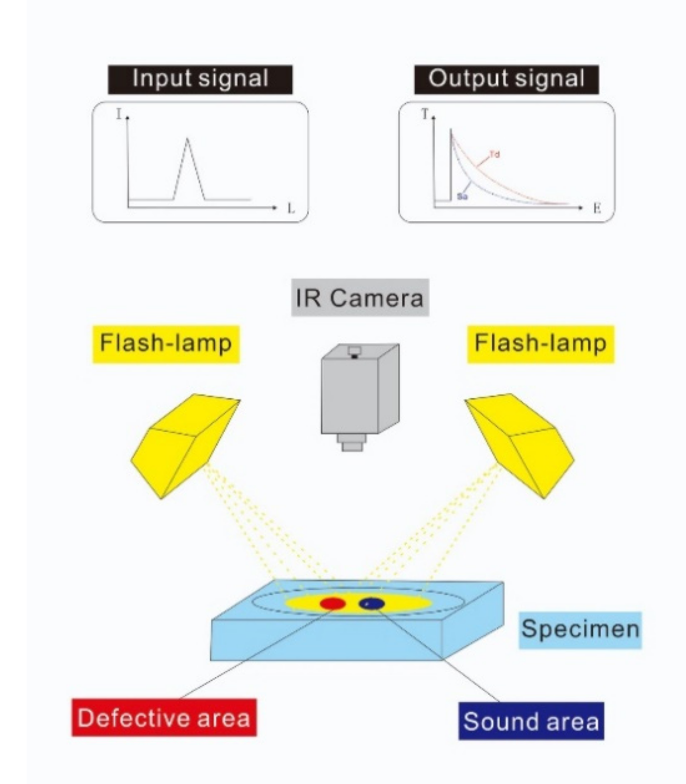
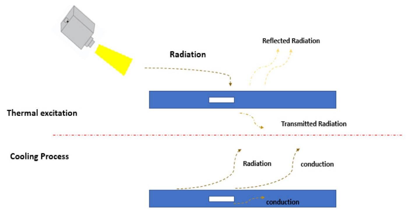
2.1. Pulsed Thermography

In pulsed thermography (PT), a high-power exponential heating impulse is applied to the samples, and a thermal response is measured during a period of time. Due to the heat conduction, a surface region which has an internal defect underneath the surface perturbs the thermal waves propagation on the surface of specimens in comparison to the sound (non-defective) region. We can then see the changes of the temperature variation, since the internal defects possess different thermo-physical (conductivity, density and heat capacity) that have an impact on heat flow. These thermal differences can be observed as surface features and recorded with an infrared camera as indicated in Figure 1 [10].
Temporal evolutions can be observed from the defective regions and subsurface sound regions. A thermal contrast is acquired as a feature vector which is obtained distinctly via the thermal value from the defective region subtracted from the corresponding value from the surrounding sound region [11] as indicated in Equation (1), where Td(t) is the temperature value on the pixel point of the defect area. The temperature value on the reference point of the sound area is T s t Then the ΔT(t) is the absolute thermal contrast extracted from the defect and sound region. The thermal contrast is an excellent technique to distinguish the temperature difference to learn the depth of the defects, as shown in Figure 1.
Δ T ( t ) = T d t T s t

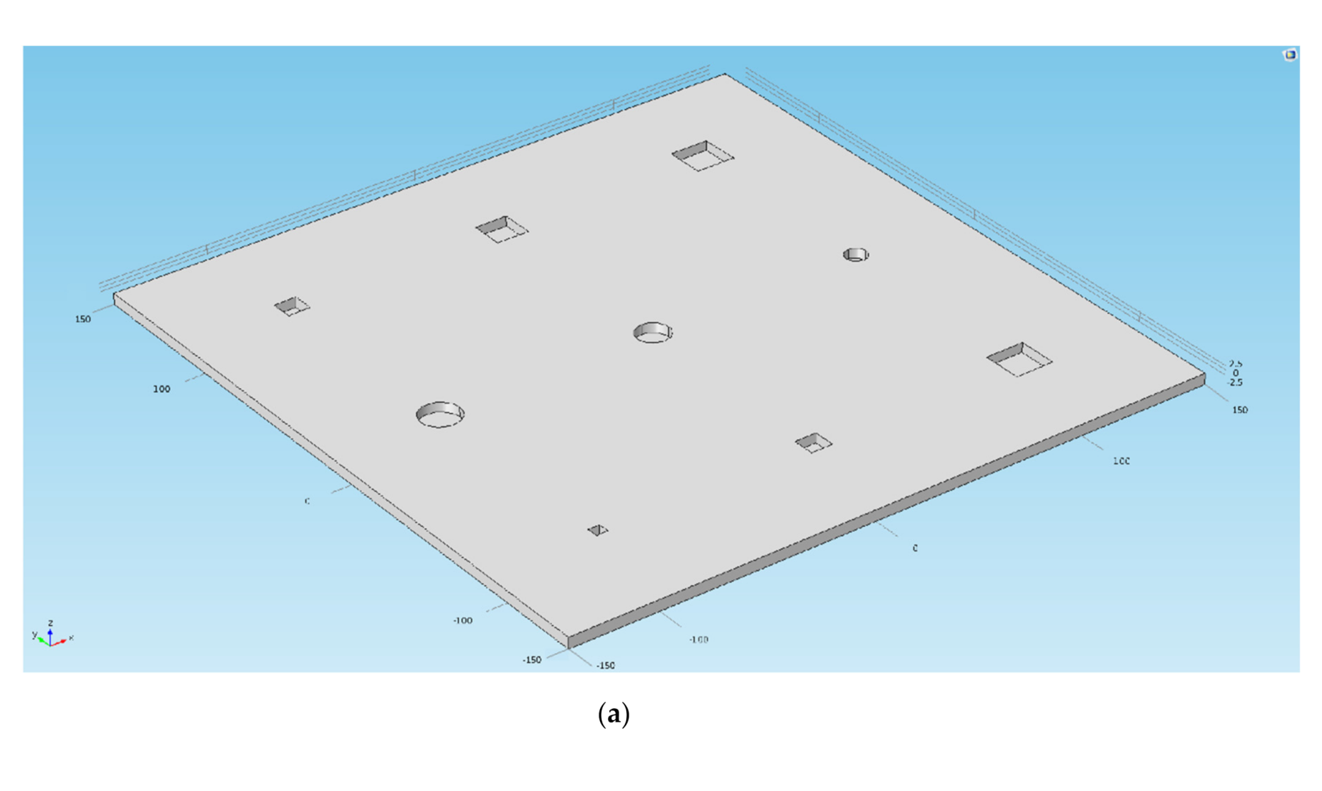
2.2. Finite Element Modeling with Transient Heat Transfer

Finite Element Modelling (FEM: COMSOL, etc.) [12] has become an important and economical platform to evaluate the thermal response of pulsed thermography, which builds up models for the platform of components that allow us to flexibly examine all specific physical aspects of thermal data such as geometries and properties of materials. Simulated thermograms matched well with experimental data.
In this work, COMSOL will be utilized as a 3D based simulation to build up models for the synthetic data to provide for depth estimation of artificial defects. A Carbon Fiber Reinforced Polymer (CFRP) structure-based specimen containing artificial defects of different shapes (flat-bottom holes) is modeled as shown in Figure 2. A high thermal pulse is projected on the surface of specimens. Due to the existence of the temperature gradients in the sample, a thermal front propagates from the high temperature region on the surface to the region underneath. A delamination or discontinuities create a lower thermal diffusion rate to the heat flow and then reflect the unnormal thermal patterns on the surface. The COMSOL software is utilized as the heat transfer simulation model for obtaining the temperature evaluations of the surface of each sample, as indicated below [13]:
ρ C P T t   · k T = 0
x w x T x + y w y T y + z w z T z = ρ C P T t
n · w · T = h c o n v T a m b T + σ T c ε T a m b 4 T 4
where in Equations (2)–(4), the density is ρ k g m 3 , constant specific heat is c ρ J k g . m , and the absolute temperature is T(K). Time variable is set as t(s). A rectangular coordinate system (x, y, z) as in Equation (3) in anisotropic media can lead to numerous possible solutions. w,   w x ,   w y ,   w z w m . K are the main conductivity rates and conductivity rates which respectively for three coordinates (x, y, z) in 3D thermal modeling. The convection heat transfer is given by h c o n v   w m 2 k . In Equation (4), a boundary condition that regarding to the thermal heat transfer from radiation and convection between the all the specimen surfaces and the ambient temperature has been indicated, where T a m b is an initial environment temperature which consider all the external environment as the same temperature; σ T c w m 2 k 4 is the Stefan–Boltzmann physical constant which links the temperature with energy; ε represents surface emissivity.
COMSOL’s heat transfer module are adapted in this work which uses the 3D transient heat equation and provides the specimen temperature distribution, to simulate the specimen’s thermal response after a heat pulse is applied to the specimen surface. A Gaussian power density distribution was employed to model the heat source, which closely approximates a real heat pulse from two flashes, i.e., a slightly larger heat accumulation at the center of the specimen. The heat pulse is applied as a radiative source that is partly absorbed by the specimen surface and transferred inside the specimen by heat conduction.
Table 1 briefly illustrates the physical properties of CFRP specimens and pulsed thermography parameters involved in the COMSOL simulation in this experiment. All properties and parameters in Table 1 are cited from the literature [14]. In this table,   T i is the initial temperature of an experimental specimen that was texted by PT. t e n d means the whole cooling processing to observe the temperature evaluation after the heating pulse application, also means the process time to finish computations. The time step is 0.0063 (the framerate: 158 frame/second). In this FEM stimulation, three types of heat flux transformation (radiation; convention; conduction) occurring during the thermal excitation period and cooling process are illustrated in Figure 2.
Table 2 and Table 3 provide the description of defect characteristics including the depth, size, shape of each defects, which characterized respectively two different group samples for training and testing. The training group has six CFRP samples (30 cm × 30 cm). Each sample has a different geometric distribution, depth, and size of defects.
Each row in every CFRP samples has the same depth of defect, which included 22 different constant values from 0.5 mm to 2.2 mm to be set from the first row in training sample 1 to the last row in training sample 6. We extracted five vectors from each defect region for GRU model training with depth estimation. The testing group has four CFRP samples (30 cm × 30 cm).
In order to differ from the training samples, the testing group consists of samples A, B, C, D. The depth of defects in the test samples ranges from [0.5 mm, 2.2 mm] but has a size that differs from that of the training samples. The CFRP geometrics of the structure of training sample 1 is indicated in Figure 3.

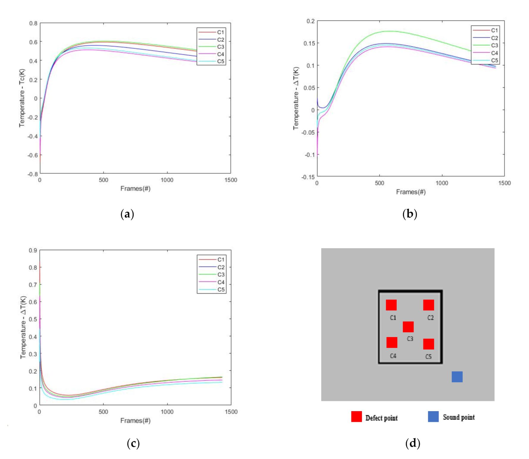
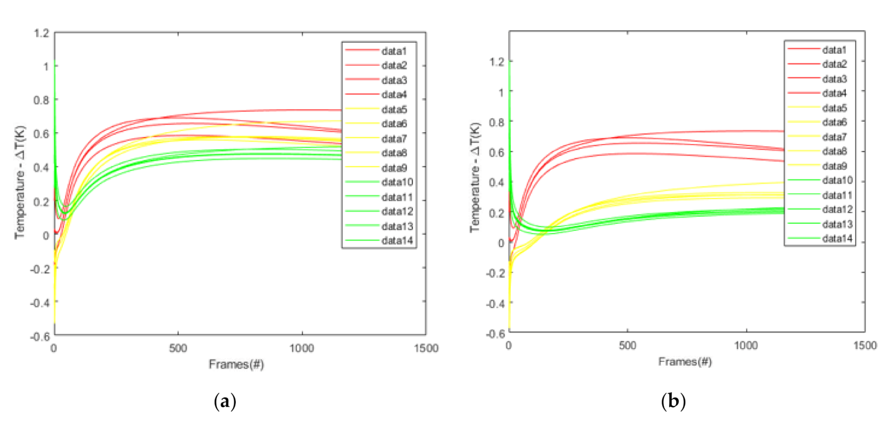
2.3. Temperature and Thermal Contrast Curves

In transient thermography, previous researchers [6] concluded that the time t c that corresponds to the maximum temperature contrast ΔT has an approximately proportional relationship with the square of the depth of the defect ( d 2 ). Simultaneously, the proportionality coefficient of this relationship rested with the lateral size of the depth: the smaller the defects, the lower the maximum contrast ∆T and earlier peak time. As indicated in Figure 4, an interesting case is highlighted. We observed the temperature evaluation of three defects of the same size (18 mm × 18 mm) but different depth such as (0.5 mm, 1.0 mm, 1.5 mm). Although the three defects have the same shape, it can be demonstrated that the shallower the defect, the higher the peak temperature value which can be obtained.
In this work, five contrast vectors have been extracted above each defect region on the surface from the different points in the defects to reduce the inaccurate influences caused by the small temperature variation. In Figure 5d as indicated in the below, in each defect region, the red cube is a defect point which localized on the corner of the upper left (C1); upper right (C2); center (C3); lower left (C4); lower right (C5). The blue cube is the reference point with respect to each defect point that we extracted. In Figure 5a–c, the data distribution of the thermal contrast curves is illustrated. C1-C5 are thermal contrasts that extracted from each defect point (in Figure 5d) based on the temperature difference between the defect point and reference sound point.
Notice that each training sequence to be processed in this work are extracted from the three quarters frames in the total frames of the one thermal sequence which already include the information of peak thermal contrast T m a x and corresponding t _ m a x . As a result, the last quarter frames of thermal curves were not extracted in this work which would show a dramatic decrease of the thermal contrasts in the graphs. To be notice that, all the thermal sequence stimulated from the COMSOL software based on the parameters as indicated on Table 2. All the extraction work was implemented in a program in MATLAB software. This partial extraction in thermal data could save the computational expense for the training in GRU to some extent.
A corresponding synthetic thermogram frame for training sample 2 in t = 3 s generated from COMSOL is indicated at in Figure 6a; nine artificial flat bottom Figure 6b hole defects were embedded with different depths in the shapes of either circles or squares.

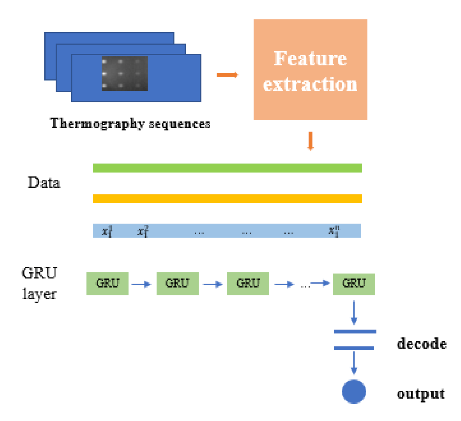
3. Proposed Strategy for Defect Depth Estimation

In this section, a defect depth estimation strategy has been proposed to detect and identify the depth of each defect in thermal images as indicated in Figure 7. This design of detection system originated from the GRU neural network. The infrared thermal module and simulations are provided by COMSOL (FEM simulation) to examine the depth of defects in pulsed thermography (PT). First, the synthetic thermal sequences are acquired from FEM (COMSOL) based on the heat transfer modeling in FEM. Then, several thermal contrast feature vectors are extracted from each defect region to feed into the input of GRU. The output of GRU consists of a unique node which estimated the depth during the training. The mean absolute error is chosen as the loss function with the GRU model in the equation as below Equation (5). In the end, the predicted depth output from the GRU is based on the feature extraction of thermal contrast vectors.
L c o s t = i = 1 m y y ^ 2 m
The GRU takes each vector at a time point in the input. This learning model was trained for 2500 epochs of each process. The training loss converged to the optimistic value and then flattened. In addition, the number of training curves (batch size) is set m. y ,   y ^ are the ground truth and estimated depth respectively.

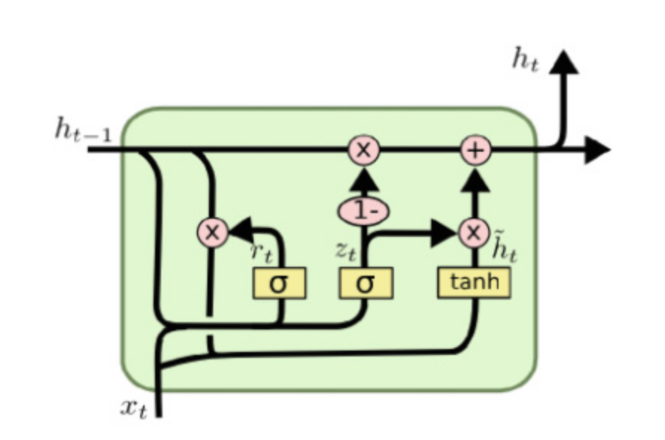
Gated Recurrent Unit Model with Depth Estimator

Due to the time continuity of the thermal sequence, each frame collected from the experiment is related to the recent historical frame, therefore the time series memory deep learning model can be applied to the thermography data based on this feature. The GRU model is originally from RNN which is a time series model that can handle the continuous information such as thermal sequences [15]. During the cooling period of the thermal data, the temperature evaluation curves over time are acquired from the given infrared frames. The learned GRU model is able to distinguish whether the pixel is from a defective region or a sound region due to the training period. Therefore, the multiple units of GRU could be applied to extract the features of the temperature evaluations from the samples based on physical properties.
The GRU neural network in Figure 8 are structured as follows [16]. In Equations (6)–(9), R t , Z t represent the update, reset gate units respectively. S z ,   S r , S are the weight factors for each gate unit.   x t is the current input.   h t 1 is the input from the previous time step in the hidden state. h t is the input of current memory from the hidden state. U z , U r , U o are the weight factors for previous time information h t 1 . σ . represents the sigmoid function. ° is denoted as the Hadamard product [17].
Z t = σ S z x t + U z h t 1
R t = σ S r x t + U r h t 1
h t = t a n h S z t + R t ° U o h t 1
h t = Z t ° t a n h + 1 Z t °   h t
As shown in Figure 9, in this work, the original thermal sequences were reshaped into vectors. The particular thermal contrast vectors are directly fed into the input of the GRU network structure. Each thermal contrast vector in the defect region is decoded with the depth value of corresponding defect at the output of GRU based on the thermal properties from the training sequences. In order to select the points for the simulated thermal sequences to extract temperature curves vectors, 5 different locations inside each defect surface in these defective areas were selected. Since the temperature of the defect region is not even, these selected points accounted for small temperature variations and change above each defect surface region. Each thermal contrast vector is vectorized with the same length in the time of the thermal sequence. Therefore, the input values of GRU are fed into the particular thermal contrast vectors. The output from the decode section (to be connected with the fully connected layer) are set with the corresponding defect depth of each vector. The estimated depth values in the defect region output from GRU are based on the thermal properties from the training sequences.

4. Experimental Validation and Results

4.1. Inference and Training

In this research, the training processing on GPU (NVIDIA GeForce GTX 1080Ti) took about 30 min. The operating system was set as: Ubuntu 14. 04. CPU: i7-5930k. Memory: 64 GB. Adam was introduced as optimizer.
The whole training process was also conducted using the Adam optimization. Some main hyper parameters and training parameters are set as below: weight decay 0.0001, the learning rate 0.001 and learning momentum 0.9. In this work, the temperature variety and contrast reflect on each vector. Therefore, the LSTM time step was set to 1429 (1429 frames as a time step as input).

4.2. Data Processing

To reduce the overfitting issue, the cross-validation verification method is proposed in this study. First, we collected 270 thermal contrast curves from the simulation data (5 thermal contrast curves extracted from each defect averagely). Then, we shuffled all of the data and spilt 80% of the data to train with the GRU model, while 20% were utilized to validate the performance of the GRU.
All obtained training data (the thermal contrast evaluation curves) were normalized and truncated as a fixed length of duration. Simultaneously, the input data were normalized by subtracting from the mean value of the thermal curves ( μ T c ) and dividing by the standard deviation of thermal contrast ( σ T c ) using Equation (10).
T c , n i ^ t = T c ^ t μ T c σ T c

4.3. Depth Estimation Results and Validation

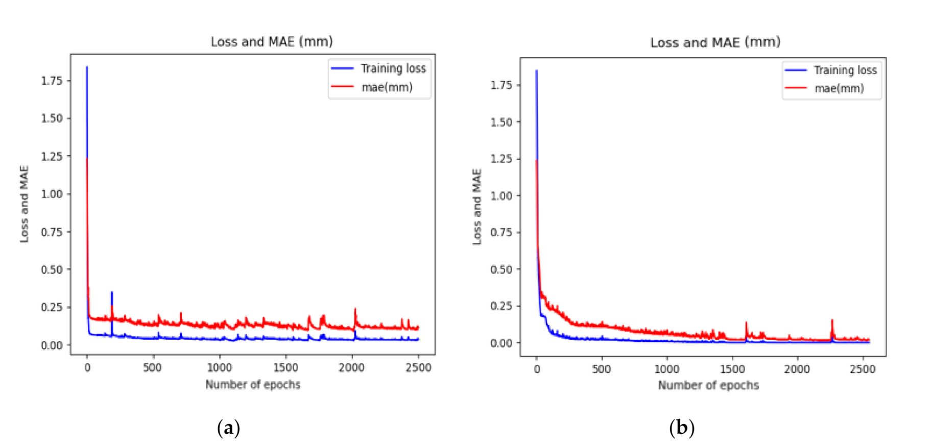
Result Analysis—Mean Absolute Error (MAE)

In statistics, the mean absolute error (MAE) [18] is one of the metrics to evaluate how close the forecasts are to the eventual outcomes. In the machine learning field, it can indirectly reflect the accuracy and performance of the machine learning model (GRU). In this work, we adapted the MAE to assess the performance of the GRU for depth estimation with infrared thermography. As we can see from Figure 10a, we trained the GRU to estimate the data from testing before the data normalization. The obtained training loss was 0.055. The MAE converged to 0.0165 mm. The error between the predictive value and actual value was within the range of 0.17   m m ,   0.17   m m . After the standard deviation normalization for all the distributed data in Figure 10b, the predictive value tended to approach the actual depth for the defect. The MAE error shrank to the range of 0.11   m m ,   0.11   m m and the training loss converged to 0.0295. This showed an acceptable performance with an improved estimate of the depth by the GRU model with standard deviation normalization.
In Table 4, the estimated output 1 and the MAE 1 were obtained from raw data without normalization (average values over the two estimated outputs from CFRP specimen groups: (A, C); (B, D)). Then, the estimated output 2 and the MAE 2 resulted from raw data of the same procedure but with normalization.
Based on Table 2, the calculated accuracy in the GRU model for the depth estimation reached 90% before data normalization (standard deviation). After normalization, the results provided an accuracy greater than 95%. This performance demonstrated that the GRU enabled a high performance for accurate depth estimation. This estimation is attributed to the ideal environment without experimental issues (noise; defective pixels). As shown in the Figure 11 below, the thermal data distribution from training (before; after) normalization has been indicated. In the data distribution (a), each group of color data curves (yellow; red; green) represents a different specific depth from defects. The thermal data were normalized by Equation (10) in Figure 10b. The distinguishable features of difference between the depths were recognized by the following principle: shallow defects had greater maximum thermal contrasts that occur earlier than deep defects. These results outperformed the previous works obtained from [7] for depth estimation in automated infrared thermography with regular neural networks.

5. Conclusions

This work elaborated the complicated and non-linear issues of evaluating defect depths in composite materials via infrared thermography with a GRU learning model. The methodology proposed here employed a GRU model combined with pulsed thermography to analyze the depth of defects. The simulated samples provide an economical platform for GRU training and depth estimation. Quantitative analysis of defect depth (subsurface features) has been evaluated by a GRU based statistical method through developed neural network modeling and cross validation experimental verification. It has been proven that the GRU modeling can produce an advanced depth detection. For future work, the experimental data have to be evaluated for the robustness of the GRU model. Further, other types of deep learning models and modified versions of the GRU model have to be applied to increase the depth estimation ability in this topic.

Author Contributions

Q.F.; conceived and designed the experiments, Q.F.; proposed the methodology, Q.F.; performed the experiment, Q.F.; performed the data analyses and wrote manuscript, X.M.; reviewed and edited manuscript, X.M.; supervised the project. All authors have read and agreed to the published version of the manuscript.

Funding

This research received no external funding.

Acknowledgments

This research is conducted under the Tier One - Multipolar Infrared Vision Canada Research Chair (MIVIM) in the Department of Electrical and Computer Engineering at Laval University. Authors would also like to thank the Chinese Scholarship Council for their financial support and help.

Conflicts of Interest

The authors declare no conflict of interest.

References

  1. D’Accardi, E.; Palano, F.; Tamborrino, R.; Palumbo, D.; Tatì, A.; Terzi, R.; Galietti, U. Pulsed phase thermography approach for the characterization of delaminations in cfrp and comparison to phased array ultrasonic testing. J. Nondestruct. Eval. 2019, 38, 20. [Google Scholar] [CrossRef]
  2. Rajic, N. Principal component thermography for flaw contrast enhancement and flaw depth characterisation in composite structures. Compos. Struct. 2002, 58, 521–528. [Google Scholar] [CrossRef]
  3. Martin, R.E.; Gyekenyesi, A.L.; Shepard, S.M. Interpreting the results of pulsed thermography data. Mater. Eval. 2003, 61, 611–616. [Google Scholar]
  4. Shepard, S.M.; Lhota, J.R.; Rubadeux, B.A.; Wang, D.; Ahmed, T. Reconstruction and enhancement of active thermographic image sequences. Opt. Eng. 2003, 42, 1337–1342. [Google Scholar] [CrossRef]
  5. Weng, J.; Zhang, Y.; Hwang, W.S. Candid covariance-free incremental principal component analysis. IEEE Trans. Pattern Anal. Machine Intell. 2003, 25, 1034–1040. [Google Scholar] [CrossRef] [Green Version]
  6. Sun, J.G. Analysis of pulsed thermography methods for defect depth prediction. J. Heat Transf. 2006, 128, 329–338. [Google Scholar] [CrossRef]
  7. Darabi, A.; Maldague, X. Neural network-based defect detection and depth estimation in TNDE. Ndt E Int. 2002, 35, 165–175. [Google Scholar] [CrossRef]
  8. Chung, J.; Gulcehre, C.; Cho, K.H.; Bengio, Y. Empirical evaluation of gated recurrent neural networks on sequence modeling. arXiv 2014, arXiv:1412.3555. [Google Scholar]
  9. Hochreiter, S.; Schmidhuber, J. Long short-term memory. Neural Comput. 1997, 9, 1735–1780. [Google Scholar] [CrossRef] [PubMed]
  10. Zissis, G.J. Infrared technology fundamentals. Opt. Eng. 1976, 15, 156484. [Google Scholar] [CrossRef]
  11. Saeed, N.; Abdulrahman, Y.; Amer, S.; Omar, M.A. Experimentally validated defect depth estimation using artificial neural network in pulsed thermography. Infrared Phys. Technol. 2019, 98, 192–200. [Google Scholar] [CrossRef]
  12. Peeters, J.; Steenackers, G.; Ribbens, B.; Arroud, G.; Dirckx, J. Finite element optimization by pulsed thermography with adaptive response surfaces. In Proceedings of the 12th International Conference on Quantitative Infrared Thermography (QIRT), Bordeaux, France, 7–11 July 2014. [Google Scholar]
  13. Lopez, F.; de Paulo Nicolau, V.; Ibarra-Castanedo, C.; Maldague, X. Thermal–numerical model and computational simulation of pulsed thermography inspection of carbon fiber-reinforced composites. Int. J. Therm. Sci. 2014, 86, 325–340. [Google Scholar] [CrossRef]
  14. Pilling, M.W.; Yates, B.; Black, M.A.; Tattersall, P. The thermal conductivity of carbon fibre-reinforced composites. J. Mater. Sci. 1979, 14, 1326–1338. [Google Scholar] [CrossRef]
  15. Chung, J.; Gulcehre, C.; Cho, K.; Bengio, Y. Gated Feedback Recurrent Neural Networks. 2015. Available online: http://proceedings.mlr.press/v37/chung15.pdf (accessed on 28 September 2020).
  16. Gulcehre, C.; Cho, K.; Pascanu, R.; Bengio, Y. Learned-Norm Pooling for Deep Feedforward and Recurrent Neural Networks. In Lecture Notes in Computer Science; Springer: Berlin/Heidelberg, Germany, 2014. [Google Scholar]
  17. Horn, R.A. The hadamard product. Proc. Symp. Appl. Math. 1990, 40, 87–169. [Google Scholar]
  18. Kassam, S. Quantization based on the mean-absolute-error criterion. IEEE Trans. Commun. 1978, 26, 267–270. [Google Scholar] [CrossRef]
Figure 1. Pulsed thermographic testing using optical excitation.
Applsci 10 06819 g001
Figure 2. Heat transfer during the thermal excitation and cooling process during FEM stimulation.
Applsci 10 06819 g002
Figure 3. Representative CFRP training sample 1 configuration
Applsci 10 06819 g003
Figure 4. Temperature contrast evaluation for defects located at different depths with the same size (0.5 mm, 1.0 mm, 1.5 mm) in training samples (the framerate: 158 frame/second).
Applsci 10 06819 g004
Figure 5. Data distribution of temperature contrast evaluation for different depths in training samples (a) 0.5 mm; (b) 1.0 mm; (c) 1.5 mm (the framerate: 158 frame/second); (d) five defective point with corresponding reference point on a defect region.
Applsci 10 06819 g005
Figure 6. (a) 3D printed defects geometrics are highlighted in training samples; (b) the corresponding synthetic colorful thermograms in t = 3 s.
Applsci 10 06819 g006aApplsci 10 06819 g006b
Figure 7. GRU model-based defects depth estimation strategy.
Applsci 10 06819 g007
Figure 8. Gated Recurrent Unit.
Applsci 10 06819 g008
Figure 9. The process of Gated Recurrent Unit (GRU) depth estimation.
Applsci 10 06819 g009
Figure 10. The mean absolute error and the training loss with GRU before (a) and after (b) standard deviation normalization.
Applsci 10 06819 g010
Figure 11. The data distribution before (a) and after (b) standard deviation normalization from all the selected locations for training (the framerate: 158frame/second).
Applsci 10 06819 g011
Table 1. Physical properties and parameters of stimulation.
SignParameters in Experimental SimulationReal Value
ρ Material density1500 k g m 3
ε Emissivity0.90
C P Constant specific heating1000 J k g . m
LSpecimen length300 mm
WSpecimen with300 mm
HSpecimen height5 mm
t e n d Processing time to finish computations9 s
T i The temperature from initialization293.15 k
T a m b The temperature from ambient293.15 k
W s o u r c e Heat source wattage600 Watts
H c e n t e r Heat source center(15 cm, 15 cm)
PHeat pulse density100,000 W m . m
hThe distance between the lamp and specimen80 cm
STime step0.0063 s
t p u l s e Heating time0.0126 s
Table 2. Defect characteristics of training samples.
SampleRowDepth(mm)ShapeDefect Size (mm)
110.5 mmQuadrangleSize = 10; 15; 18
20.6 mmRoundDiameter = 18; 15; 5
30.7 mmQuadrangleSize = 5; 10; 18
210.8 mmQuadrangleSize = 5; 10; 15
20.9 mmRoundDiameter = 18; 15; 10
31.0 mmQuadrangleSize = 5; 15; 18
311.1 mmQuadrangleSize = 5; 10; 18
21.2 mmRoundDiameter = 15; 10; 5
31.3 mmQuadrangleSize = 10; 15; 18
411.4 mmRoundSize = 5; 15; 18
21.5 mmQuadrangleDiameter = 18;10; 5
31.6 mmRoundSize = 5; 10; 15
511.7 mmRoundDiameter = 10; 15; 18
21.8 mmQuadrangleSize = 18; 15; 5
31.9 mmRoundDiameter = 5; 10; 18
612.0 mmRoundDiameter = 5; 10 ;15
22.1 mmQuadrangleSize = 18; 15;10
32.2 mmRoundDiameter = 5 ;15 ;18
Table 3. Defect characteristics of testing samples.
SampleRow#Depth (Left; Middle; Right)ShapeDefect Size (Left; Middle; Right) (mm)
A1Depth = 0.5; 0.8; 1.1QuadrangleSize = 3 ;16 ;13
2Depth = 0.6; 0.9; 1.2RoundDiameter = 8; 3; 16
3Depth = 0.7; 1.0; 1.3QuadrangleSize = 13; 8; 16
B1Depth = 1.4; 1.7; 2.0QuadrangleSize = 8; 3; 16
2Depth = 1.5; 1.8; 2.1RoundDiameter = 13; 8; 3
3Depth = 1.6; 1.9; 2.2QuadrangleSize = 16; 13; 8
C1Depth = 0.5; 0.8; 1.1RoundSize = 4; 17; 14
2Depth = 0.6; 0.9; 1.2QuadrangleDiameter = 9; 4; 17
3Depth = 0.7; 1.0; 1.3RoundSize = 14; 9; 4
D1Depth = 1.4; 1.7; 2.0RoundSize = 9; 4; 17
2Depth = 1.5; 1.8; 2.1QuadrangleDiameter = 14;9;4
3Depth = 1.6; 1.9; 2.2RoundSize = 17; 14; 9
Table 4. The results of depth estimation of defects located in the designated specimen.
SampleExpected Output (mm)Estimated Output 1 (mm)MAE1 * (mm)Estimated Output 2 (mm)MAE2 * (mm)
A C0.50.5220.0220.5070.007
A C0.60.6040.0040.6030.003
A C0.70.7080.0080.7060.006
A C0.80.8140.0140.8070.007
A C0.90.9120.0120.9130.013
A C1.01.0410.0411.0250.025
A C1.11.1090.0091.0110.011
A C1.21.2220.0221.2180.018
A C1.31.3180.0181.3140.014
B D1.41.4200.0201.4180.018
B D1.51.5140.0141.5090.009
B D1.61.6300.0301.6190.019
B D1.71.7180.0181.7150.015
B D1.81.8200.0201.8170.017
B D1.91.9180.0181.9200.020
B D2.02.0130.0132.0050.005
B D2.12.1120.0122.0100.010
B D2.22.2250.0252.2220.022
* MAE means mean square error. An average over sample for absolute different between actual and predicted observation.

