The Effect of Weather in Soccer Results: An Approach Using Machine Learning Techniques

Abstract

The growing popularity of soccer has led to the prediction of match results becoming of interest to the research community. The aim of this research is to detect the effects of weather on the result of matches by implementing Random Forest, Support Vector Machine, K-Nearest Neighbors Algorithm, and Extremely Randomized Trees Classifier. The analysis was executed using the Spanish La Liga and Segunda division from the seasons 2013–2014 to 2017–2018 in combination with weather data. Two tasks were proposed as part of this study: the first was to find out whether the game will end in a draw, a win by the hosts or a victory by the guests, and the second was to determine whether the match will end in a draw or if one of the teams will win. The results show that, for the first task, Extremely Randomized Trees Classifier is a better method, with an accuracy of 65.9%, and, for the second task, Support Vector Machine yielded better results with an accuracy of 79.3%. Moreover, it is possible to predict whether the game will end in a draw or not with 0.85 AUC-ROC. Additionally, for comparative purposes, the analysis was also performed without weather data.

1. Introduction

Soccer is considered the most popular team sport with about 250 million players all over the world. A significant amount of money circulates around this type of sport. For example, each of five best European leagues: the Premier League, La Liga, Bundesliga, Serie A, and Ligue 1 has a total wage cost of about £600 million [1]. In addition, bearing in mind the circulation of money through betting [2] makes it even more important to accurately predict the results of matches, which is important not only for betting organizations but also for fans, bettors, and stakeholders. Therefore, given the importance of the prediction of the results of soccer matches, it comes as no surprise that it has been the center of attention for years, and different techniques have been applied in order to predict the results accurately.

In the early days of this kind of research, statistical methods were mainly used to predict the results [3,4]. Nowadays, in parallel with the development of different technologies, the integration of Machine Learning (ML) techniques in the prediction analysis is increasingly more common. In view of the importance of ML technologies, Bunker and Thabtah [5] suggested a framework based on these technologies to predict sports results. Ulmer et al. [6] analyzed soccer results by implementing the following ML methods: Linear from stochastic gradient descent, Naive Bayes, Hidden Markov Model, Support Vector Machine (SVM), and Random Forest (RF). The final results showed that the Linear classifier was better than the others (with 0.48 error rates). Berrar et al. [7] proposed a new approach based on recency feature extraction and rating feature learning combined with K-Nearest Neighbors (KNN) learning and extreme gradient boosted trees (XGBoost). As an evaluation metric, the Ranked Probability Score (RPS) was used, and the results showed that XGBoost with rating features performed better (RPSavg = 0.2023). Eggels et al. [8] proposed to estimate the probability of each goal-scoring opportunity, instead of directly predicting the game result, and integration of these probabilities will give the final match result. The authors applied the following algorithms: Logistic Regression, Decision tree, RF, and a decision tree boosted with Ada-boost. The results showed that RF outperformed other techniques. Although women’s soccer is not as popular as men’s, it has still attracted the attention of researchers. One of these studies was carried out by Groll et al. [9]. The authors applied a hybrid model based on RF and two ranking methods (Poisson ranking method and abilities based on bookmakers’ odds).

It must be mentioned that the results of such studies depend not only on the methods implemented but are also more and more dependent on the features included in the analysis. Kampakis and Adamides [10] showed that the integration of data from Twitter could significantly improve the final results. In another study conducted by Shin and Gasparyan [11], the authors utilized virtual data extracted from video games for soccer result prediction.

Another important aspect is the weather conditions. These were the main subject of several studies and, although the main objective was not to predict the final result, some of them were focused on analyzing the impact of the weather on different features of the game, such as the distances run by players, injuries, successful passes, etc. For example, Landset et al. [12] tried to analyze the occurrence of injuries by considering weather conditions and the playing surface. They applied nine classifiers, and the results showed that SVM outperformed other methods. Mohr et al. [13] attempted to correlate hot conditions with the physiological and physical status of the players. Two types of conditions were taken into account for analysis: temperate and warm ambient conditions. The results showed that warm weather conditions cause the following consequences: a reduction in the distance covered in the match and high intensity running, and an improvement in peak sprinting speed and successful passes. Similar research to this last study was carried out by Nassis et al. [14], who chose 64 games in the 2014 FIFA World Cup in Brazil in order to compare environmental conditions. The datasets consisted of Wet-bulb globe temperature parameters and relative humidity recorded one hour before the game. The environmental conditions were divided into high, moderate, and low stresses. They also found that the distance covered at high intensity was also lower under high environmental stress than when such stress was low, the rate of successful passes was higher under high environmental stress, and the number of sprints was lower under high environmental stress than under moderate or low stress conditions. Orchard et al. [15] examined the relation between climatic characteristics and the occurrence of injuries. They compared the Australian Football League (AFL) with European soccer, and the main findings were that AFL teams have a higher probability of injuries in northern (warmer) areas. In contrast, European teams suffer injuries more often in northern (cooler) areas. The interesting observation derived from the latter study was related to the type of injury. The authors found that ankle sprains and anterior cruciate ligament injuries are more likely to appear in areas with warmer climates, whereas Achilles tendinopathy was more common in colder regions. Another observation was carried out by Schwellnus et al. [16] with the aim of analyzing the environmental conditions and impact of jet lag on exercise performance during the 2010 FIFA World Cup in South Africa. From their results, they tried to give valuable advice in order to prevent negative consequences of these two factors. Lucena et al. [17] analyzed variations in weather conditions after the 2014 World Cup, in Brazil. Also worth mentioning in this part is the study by Owramipur et al. [18], whose objective was to predict soccer results using the Bayesian Network model. The model was applied on the matches of Barcelona team in the 2008–2009 season. One of the factors that the authors took into account in the analysis was estimation of the weather with two categories: good and bad.

As mentioned earlier, research highlights the importance of the prediction of the results of soccer games and the influence of weather conditions on the final results; however, there is no study focusing on predicting soccer outcomes including weather data as one of the primary features. Therefore, taking into account the power of ML technologies and the importance of the weather conditions on soccer matches, the main aim of this study was to predict soccer results, as the main feature, by considering weather conditions with the help of ML technologies. In addition, the following questions were formulated as the main research questions: (a) How do weather conditions affect the results of soccer matches?; and (b) Which ML methods can predict the results of soccer matches with greater accuracy, taking the weather conditions into account as a principal feature?

The rest of the paper has the following structure: Section 2 introduces the datasets that were utilized and describes each step involved in the workflow of the applied methodology. Section 3 presents the results. Section 4 discusses the obtained results and offers the overall conclusion from the work.

2. Materials and Methods

This section describes the datasets and the methods which were applied in order to implement the analysis and answer the research questions of the current study. The core of the methodology is based on the concept and the tools provided by ML.

The main aim of this study is to predict the result of the game, which can be one of the following results: home team win, away team win, and a draw. An additional task extracted from the main objective is to find out if the result of the game will be a draw or not. On the basis of these objectives, two case studies were defined: case study 1 (home team win, away team win, and a draw) and case study 2 (a draw or not a draw), and the obtained results were compared with the outcomes of the analysis performed without weather data. It is evident that both case studies belong to supervised learning, and they are classification problems, although it should be noted that the first case study is a multivariate classification problem, and the second is a bivariate problem.

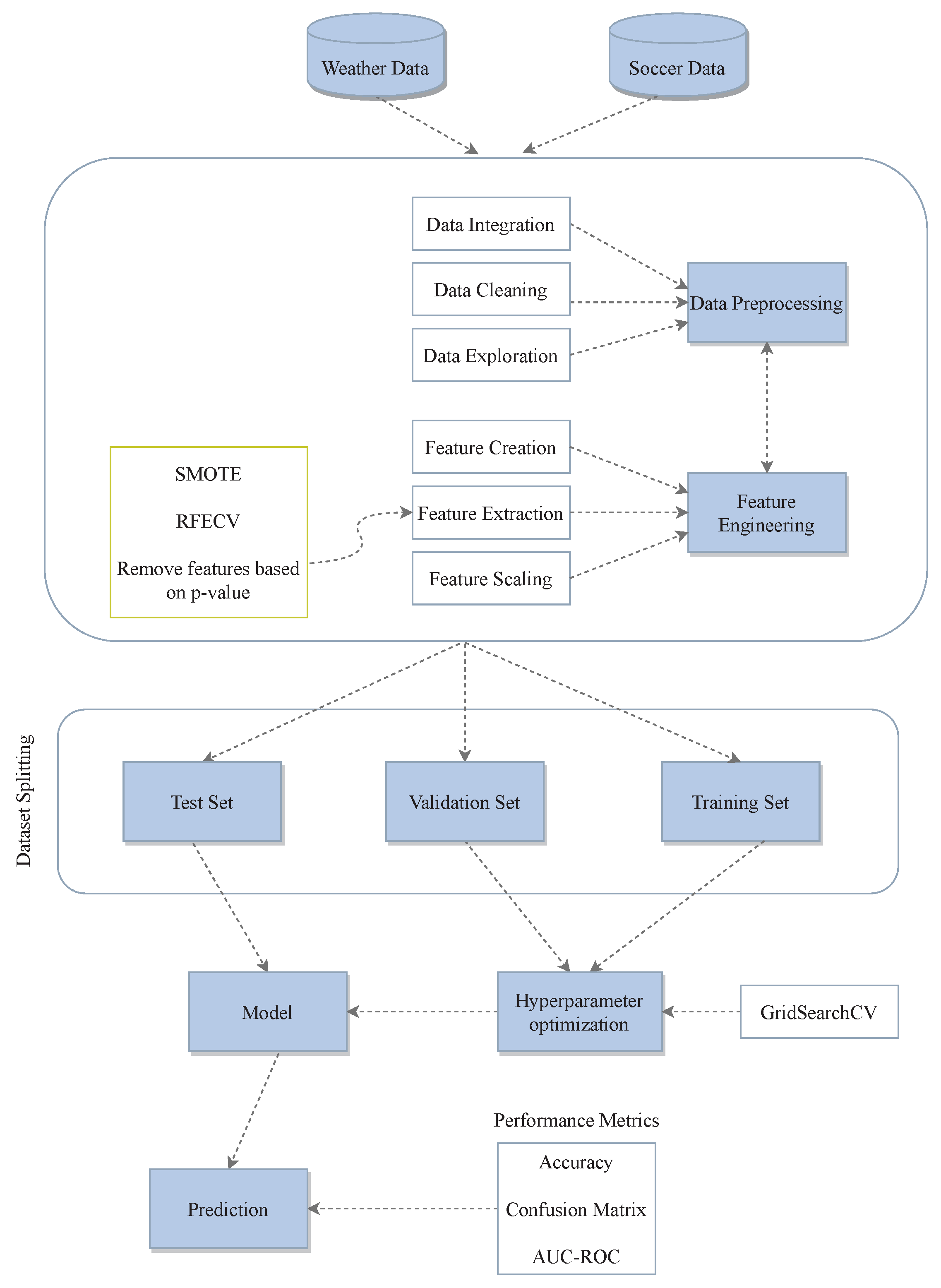
Figure 1 shows the workflow of the methodology implemented, and below it each item is described separately.

2.1. Data

The data used in this study consist of two datasets: soccer and weather. The data on soccer results are from previous matches played in the Spanish La Liga and Segunda division (La Liga 2) in the seasons 2013–2014 to 2017–2018. These are the top two divisions in men’s professional football in the Spanish football league. Overall, 20 teams compete in La Liga and 22 in the Segunda division. After each season, the three teams that finish in the lowest positions in La Liga are relegated and replaced by the two best teams and the winner of a play-off in the Segunda division. The data are available online in comma-separated values (CSV) files [19]. They include shots on goal, corners, fouls, offsides, odds (more than ten major online bookmakers, for example, Bet365, Blue Square, Gamebookers, Interwetten, Ladbrokes, William Hill odds), red cards, referees, and full-time and half-time results.

The weather data were obtained from the Agencia Estatal de Meteorología (AEMET) [20]. They include a station identifier, date, maximum temperature °C), time of maximum temperature, minimum temperature (°C), time of minimum temperature, average temperature (°C), maximum gust of wind (Km/h), the maximum gust time, maximum wind speed (Km/h), maximum wind speed time, daily total precipitation (mm), precipitation from 00.00 to 06.00 (mm), precipitation from 06.00 to 12.00 (mm), precipitation from 12.00 to 18.00 (mm), and precipitation from 18.00 to 24.00 (mm).

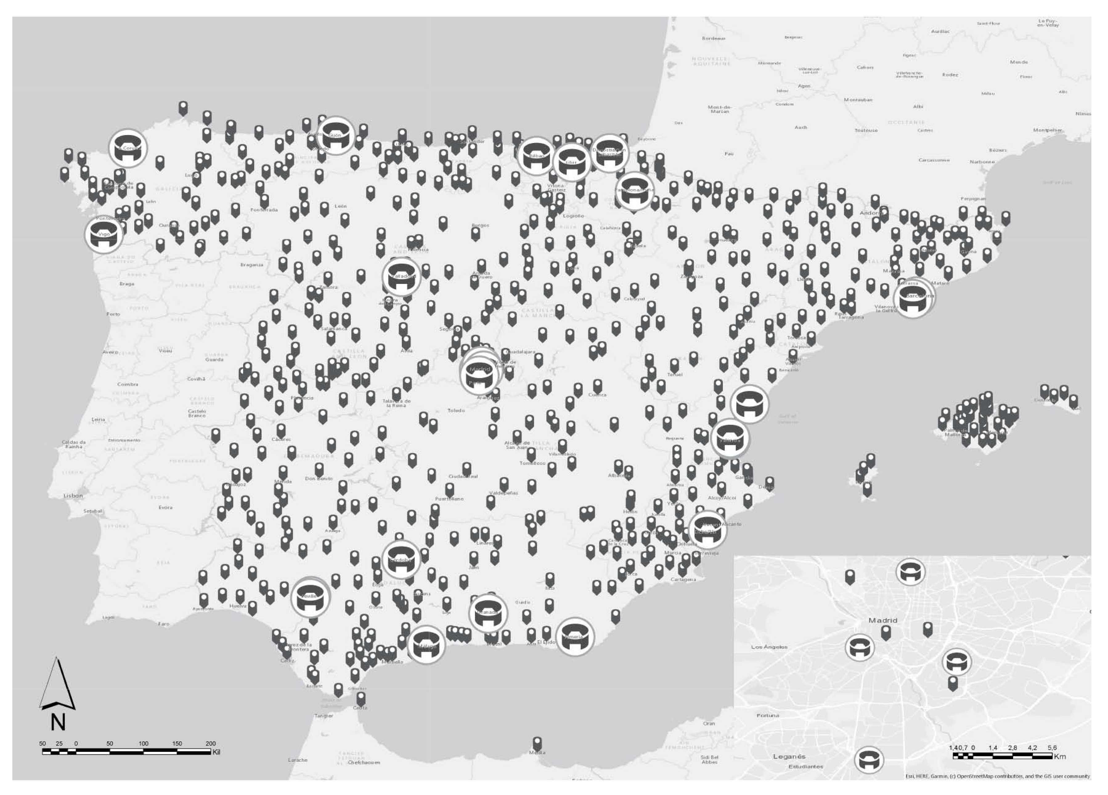
To combine two datasets, the first step was to find the nearest weather stations to the stadiums where certain football matches took place. Figure 2 shows the location of the weather stations and the stadiums in Spain. Overall, there are 775 weather stations and 25 stadiums in the selected datasets.

After finding the closest weather station, the next step was to join the two datasets using ID and Date columns. The features that were extracted for this study are dates, names of teams, odds (Bet365, Bet&Win), maximum, minimum and average temperature, precipitation, maximum gust of wind, and maximum wind speed. The dataset contains 3884 records, excluding all null values.

Table 1. Weather variables and corresponding value ranges.

Variables	Value Ranges	Variables	Value Ranges
Tmax_Home (°C)	0–42	Tmed_Away (°C)	−2–31
Tmin_Home (°C)	−8–26	Racha_Away (Km/h)	0–97
Tmed_Home (°C)	−1–32	Tprec_Away (mm)	0–95
Racha_Home (Km/h)	0–117	Vmax_Away (Km/h)	0–68
Tprec_Home (mm)	0–90	Tmed_Diff (°C)	0–30
Vmax_Home (Km/h)	0–72	Trange_Diff (°C)	0–26.8
Tmax_Away (°C)	0–39	Tprec_Diff (mm)	0–90
Tmin_Away (°C)	−7–26	Vmax_Diff (Km/h)	0–59

displays existing weather variables, new created variables using several features from an existing list and equivalent ranges, where Tmax, Tmin, Tmed are maximum, minimum, and average temperatures, Racha is maximum gust of wind, Tprec is daily total precipitation, Vmax is maximum wind speed, Tmed_Diff is the average temperature difference, Trange_Diff is the difference in temperature range, Tprec_Diff is the difference in precipitation, and Vmax_Diff is the difference in wind speed (the last four components are calculated using the home team and the away team observations).

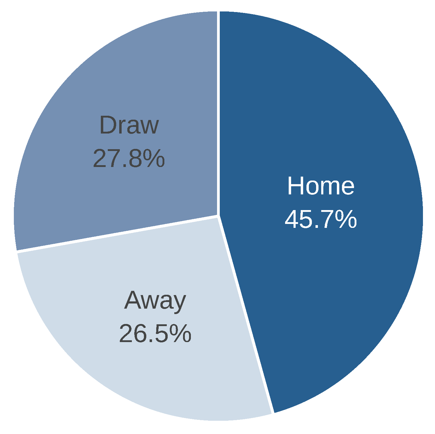
Regarding full-time results for the whole period, Figure 3 illustrates the distribution as a percentage for each case: home win, draw, and away win. It can be seen that the number of full-time results with the home team winning exceeds other results, which can be explained by the advantage enjoyed by the home team. Many studies and analyses aim to reveal the benefits of a home team [21,22]. There are many factors behind this concept, such as traveling, fans, referees, and field composition. Traveling, which is closely related to the research questions of this study (weather conditions), as well as the duration of the journey, and geographical conditions affect the performance of teams [23]. Apart from this factor, the influence of fans and referees is also very important. The shouting and noise expressed by the fans can cause low performance in the away team, but more often it can affect referees when it comes to making a decision, and it is obvious that the referees’ decisions can have a vital effect on the final result [24]. Several studies have confirmed the belief that referees are biased toward the home team [25,26]. The conditions of the playing field are also crucial, as the home team is more familiar with the environment and knows better how to play on their own pitch [27].

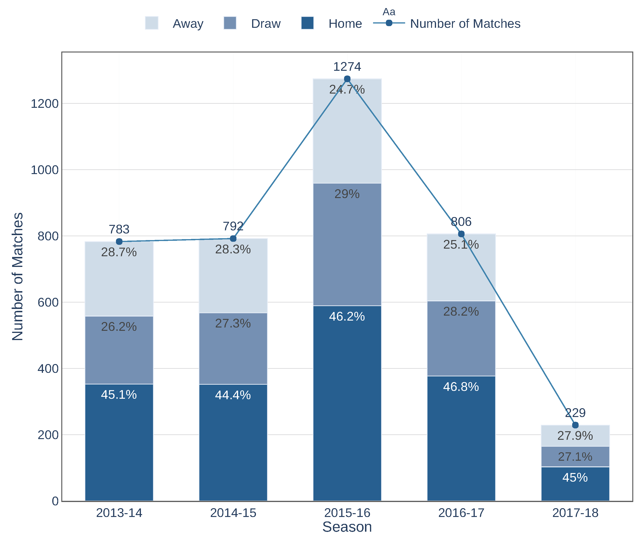
The same pattern can also be noted in Figure 4, which shows full-time results for each season. During the five seasons, the home team won more frequently. It can be observed that the number of matches during the seasons has been changed. The reason for having fewer matches for the 2017–2018 season has to do with the availability of the weather data used in this study (the soccer data were only included for matches for which complete weather data were available).

2.2. Data Preprocessing

This step includes data integration (by combining weather and soccer datasets), cleaning, and exploring the result obtained, which is described in detail in the previous section. Visualization of the entire dataset and different features was implemented, which made it possible to gain insights, to handle missing values, and to find existing outliers.

2.3. Feature Engineering

Feature engineering is the ML workflow stage that is in circular connection with data preprocessing. The following substeps were involved in feature engineering: feature creation, feature extraction, and feature scaling. After data exploration, new features were created, namely, temperature differences taking the mean and range of temperatures, precipitation differences, and the differences in wind speed between the home team and the away team.

The second component of feature engineering is feature extraction, which was performed using the Synthetic Minority Over-sampling Technique (SMOTE), Recursive feature elimination with cross-validation (RFECV), and calculation of the p-value. As seen in Figure 3, there is an imbalance between the classes. Therefore, SMOTE served to solve the problem of imbalanced classification [28]. RFECV was applied to remove the weakest features [29]. Finally, calculating the p-value helped to select features whose p-value is smaller than the defined threshold (0.05) [30] and Statsmodels was implemented in order to calculate the p-values [31]. This step is significant because selecting more representative and relevant features can prevent the scourge of dimensionality and unnecessary storage, reduce computational time, and improve accuracy [32].

The next phase was feature scaling. Depending on the ML model, feature scaling can lead to improved accuracy. Thus, before specific algorithm implementation, feature scaling was applied.

2.4. Dataset Splitting

After data preprocessing and feature engineering, it is necessary to split the data into the training and the test sets, which was carried out with ratios of 0.8 and 0.2. However, having only these two sets can lead to weak performance. The training set is the basis for training the model and fitting its parameters to the data, but it is necessary to define and determine the hyperparameters of the model. Therefore, k-fold cross-validation was applied, and in this case k was equal to five.

2.5. Hyperparameter Optimization

Hyperparameter optimization, also called hyperparameter tuning, is the process of finding optimal hyperparameters for the learning algorithm, to determine the architecture of the models in order to minimize the defined loss function. Several approaches can be used to execute this step: Grid search, Random search, Bayesian optimization, Gradient-based optimization, etc. [33]. In this study, Grid search was applied, despite several drawbacks that it has. One of these drawbacks is that it searches in a predefined search space for all possible combinations, whereas, with Random search, where the statistical distribution is specified for the hyperparameters, the values are sampled randomly. According to Bergstra and Bengio [34], not all hyperparameters are equally necessary; their significance depends on the data, and thus random search is usually preferable. However, as the study does not involve big data and there are not many hyperparameters, Grid search was chosen.

2.6. Models

To complete the tasks, the following ML methods were applied: RF, SVM, KNN and Extremely Randomized Trees Classifiers (Extra-Trees).

RF is an ensemble of Decision Trees [35]. RF trains mainly by means of the bagging method [36]. The workflow behind bagging is as follows: it first trains decision trees in randomly selected subspaces, then receives the prediction from each tree, and eventually, by combining the results, it uses voting to select the best solution. It should be noted that sampling is performed with replacement. Compared to individual trees, bagging causes a reduction in variance, which, in turn, solves the issue of overfitting.

The concept of Extra-Trees was developed by Geurts et al. [37], who described the model in detail and presented its advantages compared to other tree-based ensemble methods. Extra-Trees differs in the way it builds decision trees. It does not require bootstraping observations, and the splitting of the nodes and selection of the cut-points are performed randomly. Randomization improves accuracy and reduces the computational time; it also diminishes variance, which is an issue for other tree-based methods (Classification and Regression Trees, C4.5, etc.).

SVM aims to find a hyperplane that can classify data points. There may be multiple hyperplanes, and SVM tries to find a hyperplane with a maximum margin. The dimension of the hyperplane depends on the number of features; specifically, it is equal to the number of features minus 1. To solve the problem of finding a nonlinear decision boundary, SVM uses a kernel trick [38].

KNN is a type of lazy and non-parametric learning algorithm. It works based on the concept of proximity, especially given the belief that closer things share more similarities. The K value is used to control and adjust the proximity distance. KNN uses various distance calculation functions, such as Euclidean distance, Manhattan distance, Hamming distance, etc. The choice of a specific function depends on the data structure. One of the disadvantages of KNN is its high computational cost [39].

2.7. Prediction

To evaluate and compare the performance of ML models with the selected parameters on the extracted dataset, the prediction was executed on the test set using the following performance metrics: Accuracy, Confusion Matrix, and Area Under the Curve of Receiver Operating Characteristics (AUC-ROC).

Table 2. The possible results of the classification prediction.

	Predicted Class
		Class = Yes	Class = No
Actual Class	Class = Yes	True Positive	False Negative
	Class = No	False Positive	True Negative

displays the results that can occur as a result of the prediction, and they are the basis for the calculation of the metrics mentioned above. The results are True Positives (TP), True Negatives (TN), False Positives (FP), and False Negatives (FN), and they are the basis for the calculation of the metrics mentioned above. Our goal is to maximize TP and TN, and minimize FN and FP.

The Confusion Matrix is basically the combination of these results [40].

Accuracy (Equation (1)) is the number of correctly predicted data points from all data points [40].

$$Accuracy=\frac{TP+TN}{TP+FN+TN+FP}$$

(1)

Before explaining AUC-ROC, it is important to introduce two terms: sensitivity (also called Recall or True Positive Rate (TPR)) (Equation (2)) and False Positive Rate (FPR) (Equation (3)):

$$Sensitivity\left(TPR\right)=\frac{TP}{TP+FN}$$

(2)

$$FalsePositiveRate\left(FPR\right)=1-\frac{TN}{TN+FP}$$

(3)

Receiver Operating Characteristics (ROC) is a probability curve, and it is plotted with TPR (y-axis) against FPR (x-axis). AUC-ROC is the area under the ROC, which shows how well positive classes are separated from negative classes, and it can range from 0 to 1 [41].

3. Results

After a thorough description of the methodology and development process applied in this study, the outputs achieved will now be presented. This section presents the obtained results.

Figure 5 shows the result after applying RFECV, particularly the accuracy of classification based on the number of selected features for case study 1. It can be noted that accuracy increases, although after about nine features, it starts to vary. To know exactly which features are not important, the p-value was calculated, and features with a value greater than 0.05 were excluded.

Table 3. Variables and corresponding p-values.

Variables	P > |t|	Variables	P > |t|
Tmax_Home	0.0588	B365D	0.0000
Tmin_Home	0.1232	B365A	0.0000
Tmed_Home	0.0981	BWH	0.4560
Racha_Home	0.2068	BWD	0.4059
Vmax_Home	0.8757	BWA	0.0000
Tmax_Away	0.6878	Tmed_Diff	0.0000
Tmin_Away	0.4443	Vmax_Diff	0.0098
Tmed_Away	0.4524	Trange_Home	0.0007
Racha_Away	0.1619	Trange_Away	0.0002
Vmax_Away	0.6823	Trange_Diff	0.2831
B365H	0.0000

illustrates all the variables and their corresponding p-values for case study 1. The values in bold are features whose p-values are less than 0.05, and these features will be included in further analyses.

The same steps were also carried out for case study 2, and the final features which were used as an input to run ML models for both case studies are summarized in

Table 4. The final features of the proposed models including weather features.

Case Study 1	Case Study 2
B365H	B365H
B365D	B365D
B365A	B365A
Tmed_Diff	Tmed_Diff
Vmax_Diff	Vmax_Diff
Trange_Home	Trange_Home
Trange_Away	Trange_Away
BWA	Racha_Away

. The results of the implementation of ML techniques for both cases are illustrated below.

Table 5. Comparison of ML algorithms including weather features.

			CASE STUDY 1		CASE STUDY 2
Algorithm	Hyperparameter	Search Space	Optimal Value	Accur. (%)	Optimal Value	Accur. (%)
	Estimators	10, 50, 100, 150, 200, 250, 300, 350	300		200
RF	Min leaf	1, 5, 10, 50, 100, 200, 500	1	63.3	1	75.6
	Max features	auto, sqrt, log2	sqrt		log2
	Estimators	10, 50, 100, 150, 200, 250, 300, 350	100		250
Extra-Trees	Min leaf	1, 5, 10, 50, 100, 200, 500	1	65.9	1	76.4
	Max features	auto, sqrt, log2	auto		sqrt
	Kernels	linear, rbf	rbf		rbf
SVM	Gammas	0.1, 1, 10, 100, 500	100	64.1	500	79.3
	C	0.1, 1, 10, 100, 500	10		100
	K	3, …, 50	3		4
KNN	Weight	uniform, distance	distance	62.1	distance	71.1
	Metric	manhattan, minkowski, euclidean	manhattan		manhattan

presents the results of two case studies with the following features: Algorithm (RF, Extra-Trees, SVM, KNN), Hyperparameter (parameters that have been adjusted for each algorithm: RF and Extra-Trees: Estimators, Min leaf, Max features; SVM: Kernels, Gammas, C; KNN: K, Weight, Metric.), Search Space (the set of values for each hyperparameter), Optimal Value (the optimized value selected from the search space), and Accuracy. For comparison purposes, the same analysis was executed without weather data, and

Table 6. The final features of the proposed models excluding weather features.

Case Study 1	Case Study 2
B365H	B365H
B365D	B365D
B365A	B365A
BWA	BWA
	BWD

displays the final features serving as an input,

Table 7. Comparison of ML algorithms excluding weather features.

			CASE STUDY 1		CASE STUDY 2
Algorithm	Hyperparameter	Search Space	Optimal Value	Accur. (%)	Optimal Value	Accur. (%)
	Estimators	10, 50, 100, 150, 200, 250, 300, 350	300		250
RF	Min leaf	1, 5, 10, 50, 100, 200, 500	1	53.3	1	71.8
	Max features	auto, sqrt, log2	sqrt		auto
	Estimators	10, 50, 100, 150, 200, 250, 300, 350	150		50
Extra-Trees	Min leaf	1, 5, 10, 50, 100, 200, 500	1	52.8	1	74.9
	Max features	auto, sqrt, log2	sqrt		auto
	Kernels	linear, rbf	rbf		rbf
SVM	Gammas	0.1, 1, 10, 100, 500, 550	550	49.8	500	68.3
	C	0.1, 1, 10, 100, 500, 550	500		550
	K	3, …, 50	10		7
KNN	Weight	uniform, distance	distance	51.6	distance	71.9
	Metric	manhattan, minkowski, euclidean	minkowski		manhattan

shows the acquired results.

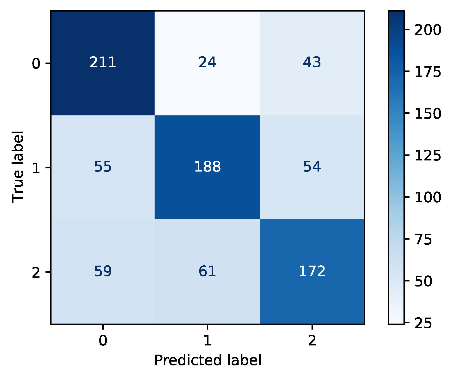
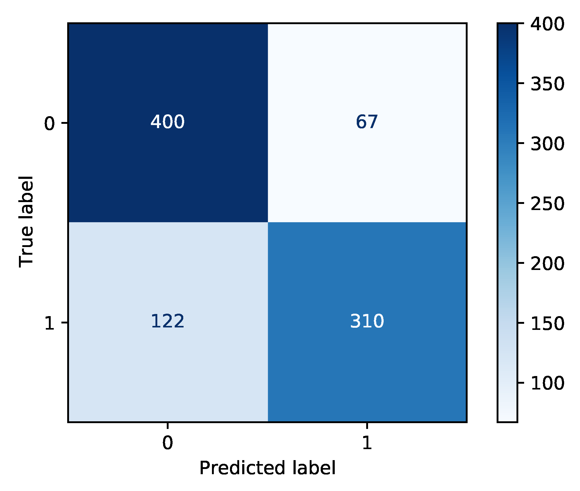
Figure 6 and Figure 7 show the confusion matrix for each outperformed method of the respective case study (case study 1: 0-away, 1-draw, 2-home; case study 2: 0-not draw, 1-draw).

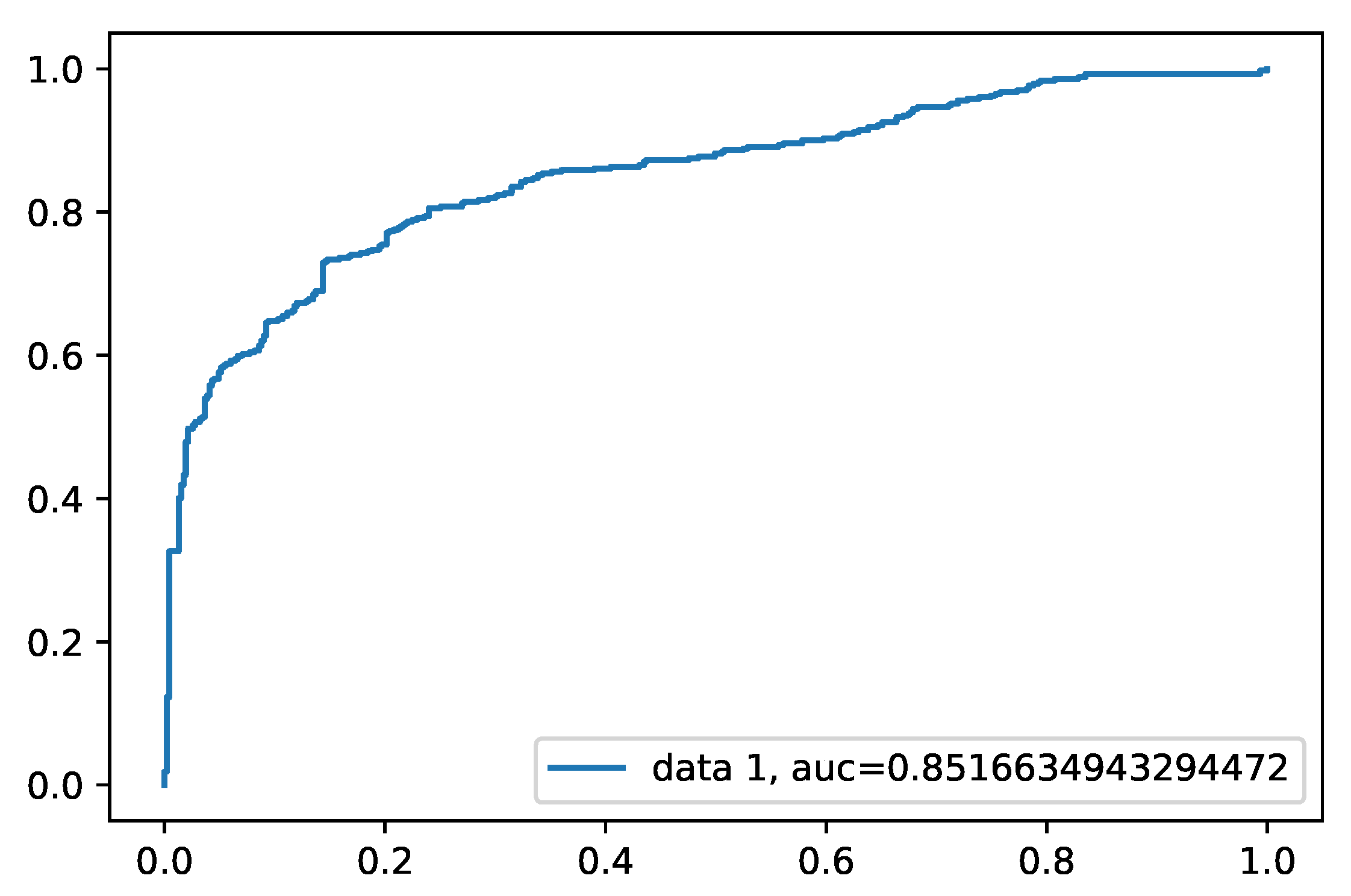
For case study 2, the area under the receiver operating characteristic was calculated. Figure 8 shows that the result is approximately 0.85.

4. Discussion and Conclusions

This work aims to predict soccer results considering the impact of weather conditions. It is evident that environmental conditions can dramatically change the output of soccer matches. Many studies have been conducted to find out the impact of weather conditions on different aspects of the game, such as injuries, speed, etc. Both financial involvement and the number of spectators are very high for this sport, and it is therefore crucial to be able to predict the result of the match with greater accuracy.

To complete the tasks addressed in this study, two case studies were set up. The first case study is to predict whether the game will result in a home team victory, an away team victory, or a draw. The second case study is to predict whether the result will be a draw or a non-draw. In order to clearly understand the importance of weather data for predicting soccer outcomes, additional analysis was performed, excluding weather data.

As previously mentioned, the following features were used in this study: dates, names of teams, odds (Bet365, Bet&Win), maximum, minimum and average temperature, difference in temperature taking the mean and the range of temperature between the home team and away team, precipitation, difference in precipitation between home team and away team, maximum gusts of wind and maximum wind speed, and the difference in wind speed between the home team and the away team.

Several techniques have been used to improve accuracy. SMOTE was applied in order to solve the problem related to the existing imbalance between classes. Later, RFECV was implemented to eliminate non-essential features. As shown in Table 4, eight features were used for each case study as final features, of which seven are the same (B365H, B365D, B365A, Tmed_Diff, Vmax_Diff, Trange_Home, Trange_Away).

After selecting and normalizing the features, the data were divided into sets for testing, training, and validation. The next step was to implement the ML methods and compare outputs. The following ML technologies were used for prediction: RF, Extra-Trees learning, SVM, and KNN.

The results show that the accuracy varies between 62.1 and 65.9 for case study 1, and between 71.1 and 79.3 for case study 2. Extra-Trees was the superior method with an accuracy of 65.9% for case study 1, and an SVM was more efficient, with an accuracy of 79.3% for case study 2. Moreover, with an AUC-ROC of 0.85, it can be predicted whether the game will end in a draw or not.

Regarding analysis carried out without weather data, the results show that the accuracy is in the range of 49.8–53.3 for case study 1, and 68.3–74.9 for case study 2. It can be noticed that RF outperformed other methods with 53.3% accuracy for case study 1, and Extra-Trees with 74.9% accuracy for case study 2.

Comparing the results of Table 5 and Table 7, it can be seen that analysis, including weather data, provides a significantly higher accuracy for case study 1. With regard to case study 2, the accuracy is also higher, except KNN, which is 0.8% lower from the results executed without weather data. The reason for this can be explained with the final features involved in the analysis presented in Table 6. It can be noticed that the final features related to betting odds are the same for case study 1 in both circumstances (with and without weather data); however, for case study 2, they differ. Therefore, it can be assumed that the analysis implemented with KNN model for case study 2, the weather data has no effect on improving the performance accuracy, while in other cases it does.

Regarding confusion matrices obtained from the analysis including weather data, it can be observed that in the first case study the higher erroneous classification was for the home-draw pair (instead of being classified as home, it was classified as draw). In the second case study, the higher misclassification was related to the classification of a non-draw, instead of being classified as a draw. The probable reason of this misclassification could be the small dataset, which in turn suggests insufficient quantity of the training data. Based on this assumption, as a limitation, the lack of data can be mentioned, considering also the fact that they are presented on a daily rate and there is no exact information at the same time when certain football matches were played. In addition, the location factor should be noted, as the weather stations are far from the stadiums and they do not provide accurate data about the stadiums.

In general, it can be concluded that integrating weather data with other features can be useful in predicting the result of a soccer match. Future work could be other types of features involvement in the analysis (for example, altitude), also the used features with more often rate can be valuable for the final output.