Data-Driven Real-Time Online Taxi-Hailing Demand Forecasting Based on Machine Learning Method

Featured Application

This research provides a valuable data-driven method on forecasting the online taxi-hailing demand, and it could be potentially applied to developing multi-modes transportation prediction.

Abstract

The development of the intelligent transport system has created conditions for solving the supply–demand imbalance of public transportation services. For example, forecasting the demand for online taxi-hailing could help to rebalance the resource of taxis. In this research, we introduced a method to forecast real-time online taxi-hailing demand. First, we analyze the relation between taxi demand and online taxi-hailing demand. Next, we propose six models containing different information based on backpropagation neural network (BPNN) and extreme gradient boosting (XGB) to forecast online taxi-hailing demand. Finally, we present a real-time online taxi-hailing demand forecasting model considering the projected taxi demand (“PTX”). The results indicate that including more information leads to better prediction performance, and the results show that including the information of projected taxi demand leads to a reduction of MAPE from 0.190 to 0.183 and an RMSE reduction from 23.921 to 21.050, and it increases R² from 0.845 to 0.853. The analysis indicates the demand regularity of online taxi-hailing and taxi, and the experiment realizes real-time prediction of online taxi-hailing by considering the projected taxi demand. The proposed method can help to schedule online taxi-hailing resources in advance.

1. Introduction

With the development of the intelligent transportation system, the travel of residents is growing more convenient. Nevertheless, because of the information asymmetry between passengers and drivers, the spatial and temporal distribution of passengers and drivers are inconsistent. The limited urban transportation resources were wasted by the information asymmetry between passengers and drivers. Therefore, trip demand in the urban area urgently needs to be studied. Recently, online taxi-hailing has gradually become the primary trip mode for urban residents. Meanwhile, the taxi still assumes the function of public transportation for urban residents. Under these circumstances, the online taxi-hailing demand would be affected by the taxi demand because of the homogeneity between the taxi and online taxi-hailing. Thus, we should take the taxi demand into account while studying the online taxi-hailing demand.

In the past, research that focused on forecasting traffic demand was mostly based on environmental data and GPS data [1,2,3,4,5,6,7,8,9,10,11,12,13,14,15,16,17,18,19,20,21,22,23,24,25,26,27,28,29,30,31,32]. Moreover, the research mined the features of GPS data and environmental data to forecast the trip demand, while the research ignored the relationship between the taxi and online taxi-hailing.

Therefore, this study aims to enhance the prediction effects of forecasting online taxi-hailing demand considering the taxi demand. Moreover, this research is a follow-up experiment of [32]. First, we use Pearson correlation analysis to screen the determinative influence factors to enhance the prediction accuracy. Then, online taxi-hailing demand forecasting models based on extreme gradient boosting (XGB) and backpropagation neural network (BPNN) were introduced to explore the relationship between taxi demand and online taxi-hailing demand. Next, we realize the real-time forecasting of online taxi-hailing demand by proposing a data-driven prediction method. This study would help to enhance the accuracy of online taxi-hailing demand forecasting and is essential for rebalancing traffic resources.

The literature review related to our study is presented in Section 2. Section 3 describes the data and the preprocessing of data in this study. Next, we proposed methods to enhance the accuracy of predicting online taxi-hailing demand in Section 4, while Section 5 concludes the results. Finally, the discussion and conclusion are shown in Section 6.

2. Related Work

Over the years, numerous works have been dedicated to enhancing the accuracy of trip demand forecasting. The first application of the trip demand forecasting is predicting trip demand based on a four-step process considering spatiotemporal factors [1]. L. Moreira-Matias et al. predicted the spatial distribution of taxi demand by presenting a method [2]. Then, he proposed a learning model considering real-time data to forecast the taxi-passenger demand’s spatiotemporal distribution [3]. Next, he proposed a combination forecasting model to forecast the taxi-passenger demand’s spatiotemporal distribution [4]. K. Zhang et al. forecasted the location of hotspots and tested the heat of the hotspots by presenting an adaptive forecasting method [5]. Next, N. Davis et al. proposed a time-series method to forecast the taxi demand by mining the regulation of taxi mobile app data [6]. X. Peng et al. forecasted the taxi demand hotspots based on social media check-ins to reduce the imbalanced supply and demand of taxis [7]. K. Zhao et al. predicted the taxi demand through three forecasting methods, respectively, based on the Markov model, Lempel–Ziv–Welch model, and ANN model [8]. Besides the GPS data and environmental data, J. Xu et al. also considered historical traffic behaviors as an important variable in the taxi demand forecasting problem, and they proposed an LSTM method to forecast taxi demand in several urban areas [9]. D. Zhang improved the hidden Markov chain model and proposed a D-model to forecast the taxi demand [10]. For exploring the relationship between taxi and subway, Y. Bao et al. took the interaction between taxi demand and subway demand into account to explore the impacts of the interaction on the accuracy of taxi demand and proposed a taxi demand prediction method based on a neural network model [11]. N. Davis explored the impacts of tessellation on-demand prediction effects and proposed a combination algorithm of different tessellation strategies to predict taxi demand [12].

The research above considered the impacts of the GPS data and the environmental data on prediction accuracy, but they did not take real-world event information into account. To address this problem, I. Markou et al. mined the real-world event information from unstructured data, and they applied the machine learning method to realize taxi demand forecasting [13]. S. Ishiguro et al. introduced the real-time demographic data into the taxi demand forecasting method and explored the impacts of demographic data on taxi demand forecasting accuracy by a stacked denoising autoencoder [14]. S. Liao conducted a comparison of two deep neural networks for forecasting trip demand and found that DNNs perform better than other traditional machine learning methods [15]. U. Vanichrujee et al. presented an ensemble method consisting of the LSTM model, GRU model, and extreme gradient boosting model (XGB) to forecast taxi demand [16]. J. Xu proposed a sequence learning method considering the historical demand to forecast trip demand [17]. H. Yao et al. presented a multi-view spatiotemporal network framework to simulate spatiotemporal relationships and forecasted the traffic demand [18]. H. Yan analyzed taxi requests and proposed a Bayesian hierarchical semiparametric model to forecast taxi demand [20]. L. Kuang introduced the unstructured data into a deep learning method to forecast the trip demand [21]. However, the methods above ignored the destination of passengers. L. Liu proposed a method to forecast the taxi demand between origin–destination pairs [22]. I. Markou introduced real-world events into the prediction method and used the data to forecast traffic demand [23]. F. Rodrigues et al. explored the relationship between drop-off points and pick-up points and proposed a spatio-temporal LSTM model to forecast the taxi demand [25]. F. Terroso-Saenz predicted taxi demand through the QUADRIVEN method based on human-generated data [26]. Y. Xu proposed a graph and time-series learning model considering the relationships between non-adjacent for city-wide taxi demand prediction [27]. H. Yu proposed a deep spatiotemporal recurrent convolutional neural network to forecast traffic flow [28]. X. Liu explored the impacts of the socio-economic, transport system, and land-use patterns on taxi demand forecasting [29]. A. Saadallah introduced the BRIGHT method, which is an ensemble of time series analysis models to forecast taxi demand precisely [30]. A. Safikhani proposed a STAR model to analyze the spatiotemporal distribution of taxis and introduced the LASSO-type penalized methods to tackle parameter estimation [31]. Recently, Z. Liu proposed a combination forecasting model considering the random forest method and ridge regression method to predict taxi demand in hotspots [32].

In general, given the relationship between different trip modes, more attempts can be justified. This study is initiated by a real-world case study to better understand the underlying relationship between the demands of different trip modes.

3. Data Description

3.1. Taxi GPS Data

We obtained the GPS data from the Xi’an Taxi Management Office in Xi’an city of China. The data include location information, vehicle state information, time information, and license plate information. Moreover, the taxi GPS data were recorded every 5 s for 30 days in November 2016 and include 40 million points which are located in Xi’an city of China. The GPS data were cleaned and selected. An instance of taxi GPS data is shown in

Table 1. An instance of taxi GPS data.

Field	Type	Sample	Comment
License plate number	String	BMvCh8nxqktd xniovIFuns	Anonymized
Time	String	1 November 2016 00:01:35	Time
Longitude	String	108.908109	WGS84 Coordinate System
Latitude	String	34.235744	WGS84 Coordinate System
Vehicle state	String	1	0: Without passenger 1: With passenger

.

3.2. Online Taxi-Hailing GPS Data

Online taxi-hailing GPS data are from Didi Chuxing GAIA Initiative, and the GPS data are located in Xi’an city of China. The dataset consists of 600 million track points, and it was recorded every 2–4 s for 30 days in November 2016. An instance of online taxi-hailing GPS data is shown in

Table 2. An instance of online taxi-hailing GPS data.

Field	Type	Sample	Comment
Driver ID	String	glox.jrrlltBMvCh8n xqktdr2dtopmlH	Anonymized
Order ID	String	jkkt8kxniovIFuns9q rrlvst@iqnpkwz	Anonymized
Time Stamp	String	1478223613 (4 November 2016 09:40:13)	Unix timestamp, in seconds
Longitude	String	104.04392	GCJ-02 Coordinate System
Latitude	String	34.04392	GCJ-02 Coordinate System

.

3.3. Environmental Data

The environmental data conclude air quality data and meteorological data. The air quality data in Xi’an city are from the official website of Green Breathing. The meteorological data in Xi’an city were derived from the National Meteorological Information Center. This study selects the hourly environmental data of Xi’an. In general, the environmental data contain 15 dimensions for the research (

Table 3. Environmental data structure description.

Data	Indicators	Description
Air quality data	AQI	Air Quality Index
	CO	The concentration of CO (μg/m3)
	NO2	The concentration of NO2 (μg/m3)
	O3	The concentration of O3 (μg/m3)
	PM2.5	The concentration of PM2.5 (μg/m3)
	PM10	The concentration of PM10 (μg/m3)
	SO2	The concentration of SO2 (μg/m3)
Meteorological data	W	Weather. 1: Sunny 2: Cloudy 3: Raining 4: Haze
	WS	Wind speed (m/s)
	TEM	Temperature (°C)
	SSD	Sunshine duration (h)
	PRE	Precipitation (mm)
	TG	Sensible temperature (°C)
	VIS	Horizontal visibility (m)

).

4. Methods

4.1. Feature Selection

Ensuring that the correlations between the features and the dependent variables are important in the prediction problem. Likewise, ensuring that the features are independent of one another is also important for improving the prediction accuracy. While modeling the forecasting method, both the features which exhibit strong, multiple collinearities and the features which have a low correlation with the dependent variable should be eliminated for enhancing the prediction accuracy. Thus, we choose the Pearson correlation analysis to test the correlation of all features and the dependent variable [33,34]. The calculation of Pearson correlation analysis is as Equation (1).

$${\mathsf{\rho }}_{\mathrm{X},\mathrm{Y}}=\frac{\mathrm{cov}\left(\mathrm{X},\mathrm{Y}\right)}{{\mathsf{\sigma }}_{\mathrm{X}}{\mathsf{\sigma }}_{\mathrm{Y}}}=\frac{\mathrm{E}\left[\left(\mathrm{X}-{\mathsf{\mu }}_{\mathrm{X}}\right)\left(\mathrm{Y}-{\mathsf{\mu }}_{\mathrm{X}}\right)\right]}{{\mathsf{\sigma }}_{\mathrm{X}}{\mathsf{\sigma }}_{\mathrm{Y}}},$$

(1)

$\mathrm{cov}\left(\mathrm{X},\mathrm{Y}\right)$ is the covariance between the features X and Y. ${\mathsf{\sigma }}_{\mathrm{X}}$ and ${\mathsf{\sigma }}_{\mathrm{Y}}$ indicate the standard deviations of the features X and Y. ${\mathsf{\rho }}_{\mathrm{X},\mathrm{Y}}$ is the correlation value of the features X and Y. The value range of ${\mathsf{\rho }}_{\mathrm{X},\mathrm{Y}}$ belongs to $\left(-1,1\right)$. If ${\mathsf{\rho }}_{\mathrm{X},\mathrm{Y}}>0$, the two features are positively correlated: if ${\mathsf{\rho }}_{\mathrm{X},\mathrm{Y}}<0$, the two features are negatively correlated. The larger absolute value of ${\mathsf{\rho }}_{\mathrm{X},\mathrm{Y}}$ indicates a stronger correlation between the features X and Y.

4.2. BPNN

Artificial neural networks (ANNs) possess attributes of learning, generalizing, parallel processing, and error endurance. These attributes make the ANNs useful in modeling complex situations. Therefore, we employ BPNN, a type of ANN, for forecasting online taxi-hailing demand in this study [35,36]. A three-layer BPNN employed in this paper is shown in Figure 1 [37]. In Figure 1, “T” indicates the information of time factors, “E” is the information of environmental factors, and “TX” represents the information of taxi demand.

The connection weights among nodes are obtained by data training in the backpropagation process. Then, it produces the minimized least-mean-square error between the true and the estimated values from the neural network’s output. First, the connection weights are assigned initial values. Then, the weights are updated based on the back-propagated error between the predicted and true output values. Assume that there are $\mathrm{n}$ input neurons, $\mathrm{m}$ hidden neurons, and one output neuron, a training process can be described as follows.

Hidden layer stage: Calculating the outputs of all neurons in the hidden layer as Equations (2) and (3).

$${\mathrm{net}}_{\mathrm{j}}={{\displaystyle \sum }}_{\mathrm{i}=0}^{\mathrm{n}}{\mathrm{v}}_{\mathrm{ij}}{\mathrm{x}}_{\mathrm{i}}, \mathrm{j}=1,2,\cdots ,\mathrm{m},$$

(2)

$${\mathrm{y}}_{\mathrm{j}}={\mathrm{f}}_{\mathrm{H}}\left({\mathrm{net}}_{\mathrm{j}}\right), \mathrm{j}=1,2,\cdots ,\mathrm{m},$$

(3)

${\mathrm{net}}_{\mathrm{j}}$ is the activation value of the $\mathrm{jth}$ node, ${\mathrm{y}}_{\mathrm{j}}$ is the output of the hidden layer, and ${\mathrm{f}}_{\mathrm{H}}$ is the activation function of a node; the activation function is the rectified linear unit function as Equation (4).

$${\mathrm{f}}_{\mathrm{H}}\left(\mathrm{x}\right)=\max \left(0,\mathrm{x}\right),$$

(4)

Output stage: The outputs of all neurons in the output layer are as Equation (5).

$$\mathrm{O}={\mathrm{f}}_{\mathrm{o}}\left({{\displaystyle \sum }}_{\mathrm{j}=0}^{\mathrm{m}}{\mathrm{w}}_{\mathrm{ik}}{\mathrm{y}}_{\mathrm{j}}\right)$$

(5)

${\mathrm{f}}_{\mathrm{o}}$ is the activation function as Equation (4). All weights are assigned random values initially and then modified by the delta rule according to the learning samples.

The three-layer BPNN above is the basic application of BPNN in online taxi-hailing demand prediction method. To find out the best network structure of BPNN for different forecasting models, we should use the grid search algorithm to determine the network structures of the models based on BPNN.

4.3. XGB

XGB is a boosting model based on a classification and regression tree (CART), which takes full advantage of the residual of a base classifier [38]. The boosting algorithm combines simple tree models to establish a more precise model, and it overcomes the influence of the interference signal. The prediction is as Equation (6).

$${\widehat{\mathrm{y}}}_{\mathrm{i}}={{\displaystyle \sum }}_{\mathrm{k}=1}^{\mathrm{K}}{\mathrm{f}}_{\mathrm{k}}\left({\mathrm{x}}_{\mathrm{i}}\right),{\mathrm{f}}_{\mathrm{k}}\in \mathrm{F}$$

(6)

${\mathrm{f}}_{\mathrm{k}}$ is the ${\mathrm{k}}_{\mathrm{th}}$ tree, K is the number of trees, and F is a set of all trees.

Suppose that $\mathrm{S}=\left\{\left({\mathrm{x}}_1,{\mathrm{y}}_1\right),\dots \left({\mathrm{x}}_{\mathrm{i}},{\mathrm{y}}_{\mathrm{i}}\right)\dots \left({\mathrm{X}}_{\mathrm{w}},{ \mathrm{y}}_{\mathrm{w}}\right)\right\}$ is a known dataset with N samples where x has L features, and y is the label of different emitters. The objective function is as Equation (7).

$$\mathrm{O}={{\displaystyle \sum }}_{\mathrm{i}=1}^{\mathrm{N}}\mathrm{l}\left({\widehat{\mathrm{y}}}_{\mathrm{i}},{\mathrm{y}}_{\mathrm{i}}\right)+{{\displaystyle \sum }}_{\mathrm{k}=1}^{\mathrm{K}}\mathrm{r}\left({\mathrm{f}}_{\mathrm{k}}\right),$$

(7)

${\widehat{\mathrm{y}}}_{\mathrm{i}}$ is the predicted value of ${\mathrm{x}}_{\mathrm{i}}$, $\mathrm{l}$ represents the difference between the true and predicted values. $\mathrm{r}\left({\mathrm{f}}_{\mathrm{k}}\right)$ is the regularized term of ${\mathrm{k}}_{\mathrm{th}}$ trees, which penalize the complexity of the model to avoid overfitting, and it could be calculated as Equation (8).

$$\mathrm{r}\left({\mathrm{f}}_{\mathrm{k}}\right)=\mathsf{\gamma }\mathrm{T}+\frac{\mathsf{\omega }}{2}\Vert \mathsf{\vartheta }\Vert ,$$

(8)

$\mathsf{\gamma },\mathsf{\omega }$ are penalty coefficients, T is the number of leaves in the tree, and $\mathsf{\vartheta }$ is leaf weight.

4.4. Evaluation Criteria

Moreover, three accuracy measures are applied to evaluate the performance of online taxi-hailing prediction. The measures are root-mean-square error (RMSE), mean absolute percentage error (MAPE) and goodness of fit (${\mathrm{R}}^2$), which are calculated as Equations (9)–(11).

$$\mathrm{RMSE}={\left({\mathrm{T}}^{-1}{{\displaystyle \sum }}_{\mathrm{n}=1}^{\mathrm{T}}{\left(\widehat{{\mathrm{C}}_{\mathrm{n}}}-{\mathrm{C}}_{\mathrm{n}}\right)}^2\right)}^{1/2},$$

(9)

$$\mathrm{MAPE}={\mathrm{T}}^{-1}{{\displaystyle \sum }}_{\mathrm{n}=1}^{\mathrm{T}}\left|\left(\widehat{{\mathrm{C}}_{\mathrm{n}}}-{\mathrm{C}}_{\mathrm{n}}\right)/\widehat{{\mathrm{C}}_{\mathrm{n}}}\right|,$$

(10)

$${\mathrm{R}}^2=\frac{{{\displaystyle \sum }}_{\mathrm{i}=1}^{\mathrm{N}}{({\mathrm{C}}_{\mathrm{n}}-\overline{ \mathrm{C} })}^2}{{{\displaystyle \sum }}_{\mathrm{i}=1}^{\mathrm{N}}{(\widehat{{\mathrm{C}}_{\mathrm{n}}}-\overline{ \mathrm{C} })}^2},$$

(11)

$\widehat{{\mathrm{C}}_{\mathrm{n}}}$, ${\mathrm{C}}_{\mathrm{n}}$ and $\overline{ \mathrm{C} }$ are the true, the predicted, and the mean value, respectively. Then, $\mathrm{T}$ is the number of samples.

5. Results

5.1. Feature Selection

Before we predict the online taxi-hailing demand, we should select a reasonable set of forecasting features. Therefore, we use Python to calculate the correlations among prediction indicators, and we eliminate factors with strong collinearity and factors with low cross-correlation. Correlations among environmental factors are as

Table 4. Correlations among environmental factors.

	OT	DW	HD	WON	AQI	PM2.5	PM10	SO2	NO2	CO
OT	1	0.23	0.79	0.22	0.06	0.06	0.07	0.02	0.08	0.08
DW	0.23	1	0	0.79	0.29	0.28	0.34	0.13	0.36	0.4
HD	0.79	0	1	0.11	0.05	0.07	0.09	0.05	0.14	0.12
WON	0.22	0.79	0.11	1	0.13	0.2	0.25	0.19	0.25	0.35
AQI	0.06	0.29	0.05	0.13	1	0.79	0.95	0.3	0.69	0.8
PM2.5	0.06	0.28	0.07	0.2	0.79	1	0.7	0.46	0.8	0.88
PM10	0.07	0.34	0.09	0.25	0.95	0.7	1	0.37	0.67	0.8
SO2	0.02	0.13	0.05	0.19	0.3	0.46	0.37	1	0.46	0.5
NO2	0.08	0.36	0.14	0.25	0.69	0.8	0.67	0.46	1	0.91
CO	0.08	0.4	0.12	0.35	0.8	0.88	0.8	0.5	0.91	1
O3	−0.18	−0.25	0.07	−0.15	−0.35	−0.53	−0.35	−0.34	−0.36	−0.47
W	−0.02	−0.17	0	−0.2	0.31	0.51	0.16	0.15	0.23	0.3
WS	0.11	−0.04	0.1	0.02	−0.02	0.13	−0.01	0.48	0.04	0
TEM	−0.39	−0.07	−0.38	−0.06	0.01	0.02	−0.06	−0.36	0	0.04
RHU	0.41	0.13	0.34	0.19	0.08	0.15	0.11	−0.11	0.18	0.2
PRE	0.02	−0.02	0	−0.02	−0.04	−0.03	−0.05	−0.05	−0.06	−0.03
SSD	0.06	0.22	0	0.18	−0.09	−0.29	0.07	0	0.19	0.03
TG	−0.23	−0.03	−0.13	−0.04	−0.09	−0.14	−0.14	−0.56	−0.11	−0.07
VIS	−0.27	−0.18	−0.17	−0.28	−0.04	−0.29	−0.06	−0.24	−0.35	−0.34
TX	0.52	0.06	0.5	0.01	0.01	0.02	0	−0.04	0.04	0.02
	O3	W	WS	TEM	RHU	PRE	SSD	TG	VIS	TX
OT	−0.18	−0.02	0.11	−0.39	0.41	0.02	0.06	−0.23	−0.27	0.52
DW	−0.25	−0.17	−0.04	−0.07	0.13	−0.02	0.22	−0.03	−0.18	0.06
HD	0.07	0	0.1	−0.38	0.34	0	0	−0.13	−0.17	0.5
WON	−0.15	−0.2	0.02	−0.06	0.19	−0.02	0.18	−0.04	−0.28	0.01
AQI	−0.35	0.31	−0.02	0.01	0.08	−0.04	−0.09	−0.09	−0.04	0.01
PM2.5	−0.53	0.51	0.13	0.02	0.15	−0.03	−0.29	−0.14	−0.29	0.02
PM10	−0.35	0.16	−0.01	−0.06	0.11	−0.05	0.07	−0.14	−0.06	0
SO2	−0.34	0.15	0.48	−0.36	−0.11	−0.05	0	−0.56	−0.24	−0.04
NO2	−0.36	0.23	0.04	0	0.18	−0.06	0.19	−0.11	−0.35	0.04
CO	−0.47	0.3	0	0.04	0.2	−0.03	0.03	−0.07	−0.34	0.02
O3	1	−0.02	0.02	−0.06	−0.13	−0.08	0.27	−0.02	0.17	−0.02
W	−0.02	1	0.06	0.04	0.08	−0.03	−0.51	−0.07	−0.19	−0.05
WS	0.02	0.06	1	−0.53	−0.2	−0.07	−0.14	−0.68	−0.02	0.01
TEM	−0.06	0.04	−0.53	1	−0.22	0.03	−0.08	0.8	0.13	−0.2
RHU	−0.13	0.08	−0.2	−0.22	1	0.11	0.09	0.12	−0.72	0.27
PRE	−0.08	−0.03	−0.07	0.03	0.11	1	−0.03	0.07	−0.01	0.05
SSD	0.27	−0.51	−0.14	−0.08	0.09	−0.03	1	0.05	−0.05	0.03
TG	−0.02	−0.07	−0.68	0.8	0.12	0.07	0.05	1	0.01	−0.13
VIS	0.17	−0.19	−0.02	0.13	−0.72	−0.01	−0.05	0.01	1	−0.16
TX	−0.02	−0.05	0.01	−0.2	0.27	0.05	0.03	−0.13	−0.16	1

. In Table 4, “OT” and “TX”, respectively, indicate online taxi-hailing demand and taxi demand, “DW” is the day of the week, “HD” represents the hour of the day, and “WON” indicates whether the day is a workday. Other features are as Table 3.

As shown in Table 4, we find that the values of correlations among AQ, AQI, PM2.5, PM10, and CO are more than 0.8. Therefore, we remove AQI, PM2.5, PM10, and CO from the predictive factors. Next, we eliminate the features whose correlation with the OT factor is less than 0.2. Predictive indicators of online taxi-hailing demand areas are shown in

Table 5. Predictive indicators of trip demand.

Information	Indicators	Description
T	DW	Day of the week. DW is in (1, 7).
	HD	Hour of day. HD is in (1, 24).
	WON	Workday or non-workday. Workday: 0; Non-workday: 1.
E	WS	Wind speed (m/s).
	TEM	Temperature (°C).
	RHU	Relative humidity (%).
	TG	Sensible temperature (°C).
	VIS	Horizontal visibility (m).
TX	TX	Taxi demand (pcu).

. Predictive indicators in Table 5 are divided into “T”, “E” and “TX”. “T” indicates the information of the time, “E” represents the environmental factors, and “TX” contains information about taxi demand.

Then, all data are proceeded through by the One-Hot Encoder function in the scikit-learn.preprocessing library. An instance of the DW indicator is shown in Figure 2.

After the encoding of indicators in Table 5, the dimension of the dataset was expanded to 58. Additionally, the first 23 days of November 2016 are taken as the training set, with the other seven days as the testing set in this study.

5.2. Data Preprocessing

In this study, we choose the Bell Tower area as the research object according to the study of Liu et al. [32], because the Bell Tower area contains the most trip demand. The Bell Tower area is a commercial area, and its traffic demand exhibits a robust tidal phenomenon. The Bell Tower area is as in Figure 3.

Then, we cut taxi data and online taxi-hailing data into time slices. The trip demand for taxi and online taxi-hailing areas is shown in Figure 4. We find that the taxi demand and online taxi-hailing demand are regular, and taxi demand decreases while the online taxi-hailing demand increases in peak hours.

5.3. Online Taxi-Hailing Demand Forecasting

Then, we forecast the online taxi-hailing demand in Bell Tower area based on the BPNN and XGB. We test the prediction effects of different indicators based on the BPNN and XGB. In the experiment, we add time factors, environmental factors, and taxi demand factors into models based on BPNN and XGB. Models with different impacting factors are shown in

Table 6. Predictive indicators of trip demand.

Model	Model Input	Model Output
Model BPNN + T	Time data	Next week’s demand
Model BPNN + T + E	Time data + Environmental data	Next week’s demand
Model BPNN + T + TX	Time data + Environmental data + Taxi data	Next week’s demand
Model XGB + T	Time data	Next week’s demand
Model XGB + T + E	Time data + Environmental data	Next week’s demand
Model XGB + T + TX	Time data + Environmental data + Taxi data	Next week’s demand

. Next, we use the grid search algorithm to adjust the hyperparameters of models based on BPNN and XGB. Moreover, the hyperparameters for the models are illustrated in

Table 7. Hyperparameter settings for the models.

Model	Hyperparameters	Value	Optimal Value
Model BPNN + T	m (hidden neurons)	{1, 2, …, 100}	67
	n (hidden layers)	{1, 2, 3, 4}	3
	activation	{‘identity’, ‘logistic’, ‘tanh’, ‘relu’}	‘relu’
Model BPNN + T + E	m (hidden neurons)	{1, 2, …, 100}	89
	n (hidden layers)	{1, 2, 3, 4}	3
	activation	{‘identity’, ‘logistic’, ‘tanh’, ‘relu’}	‘relu’
Model BPNN + T + TX	m (hidden neurons)	{1, 2, …, 100}	88
	n (hidden layers)	{1, 2, 3, 4}	3
	activation	{‘identity’, ‘logistic’, ‘tanh’, ‘relu’}	‘relu’
Model XGB + T	gamma	{0.1, 0.2, 0.3, 0.4, 0.5, 0.6}	0.4
	learning_rate	{0.1, 0.2, 0.3, 0.4, 0.5, 0.6}	0.4
	max_depth	{1, 2, …, 50}	13
	min_child_weight	{1, 2, …, 50}	12
	n_estimators	{1, 2, …, 100}	48
Model XGB + T + E	gamma	{0.1, 0.2, 0.3, 0.4, 0.5, 0.6}	0.4
	learning_rate	{0.1, 0.2, 0.3, 0.4, 0.5, 0.6}	0.3
	max_depth	{1, 2, …, 50}	11
	min_child_weight	{1, 2, …, 50}	12
	n_estimators	{1, 2, …, 100}	38
Model XGB + T + TX	gamma	{0.1, 0.2, 0.3, 0.4, 0.5, 0.6}	0.4
	learning_rate	{0.1, 0.2, 0.3, 0.4, 0.5, 0.6}	0.3
	max_depth	{1, 2, …, 50}	11
	min_child_weight	{1, 2, …, 50}	11
	n_estimators	{1, 2, …, 100}	45

. Furthermore, the results of models with different impacting factors are shown in Figure 5 and Figure 6. Additionally, the factors of “T”, “E” and “TX” are shown in Table 5.

Then we use RMSE, MAPE and ${\mathrm{R}}^2$ to test the prediction effect of the models (

Table 8. Prediction effects of BPNN and XGB.

Models	Training Set			Testing Set
	MAPE	RMSE	${\mathbf{R}}^2$	MAPE	RMSE	${\mathbf{R}}^2$
BPNN + T	0.213	26.972	0.842	0.224	28.576	0.819
BPNN + T + E	0.178	23.692	0.851	0.190	23.921	0.845
BPNN + T + E + TX	0.127	18.632	0.893	0.132	18.696	0.866
XGB + T	0.302	24.701	0.836	0.333	26.296	0.833
XGB + T + E	0.188	19.718	0.872	0.197	21.206	0.857
XGB + T + E + TX	0.129	17.797	0.887	0.139	19.193	0.865

). Table 8 shows the RMSE, MAPE and ${\mathrm{R}}^2$ of six different models’ test datasets in the Bell Tower area. Comparing the performance of predictions based on BPNN, our results show that the model “BPNN + T + E + TX” is the best-performing method for solving online taxi-hailing prediction problems. Moreover, among three predictions based on XGB, the model “XGB + T + E + TX” is the best-performing method for online taxi-hailing prediction problems.

Next, we analyze the contributions of the different sources of information. From Table 8, we can find that including information about taxi demand (“TX”) enhances the prediction effects based on BPNN and XGB. In the BPNN models, including information “E” leads to a MAPE reduction from 0.224 to 0.190, while it decreases RMSE from 28.576 to 23.921, and increases the ${\mathrm{R}}^2$ from 0.819 to 0.845. Likewise, including information “TX” leads to a MAPE reduction from 0.190 to 0.132, and it increases the ${\mathrm{R}}^2$ from 0.845 to 0.866. Meanwhile, in the XGB models, including information “E” leads to a MAPE reduction from 0.333 to 0.197 while it reduces RMSE from 26.296 to 21.206, and increases the ${\mathrm{R}}^2$ from 0.833 to 0.857. Including information “TX” leads to a MAPE reduction from 0.197 to 0.139, and it increases the ${\mathrm{R}}^2$ from 0.857 to 0.865. Additionally, the performance of the model “BPNN + T + E + TX” is the best among the six models in Table 8.

To evaluate the prediction performance of BPNN and XGB in different hours, we report MAPE and RMSE of six models in different hours. Figure 7a shows that the model “BPNN + T + E + TX” obtains the lowest MAPE among three predictions except at 6 a.m., 8 a.m., and 9 p.m. Figure 7b shows that the performance of the model “XGB + T + E + TX” is the best except at 11 a.m. and 5 p.m. From Figure 8, we know that the model “BPNN + T + E + TX” obtains the lowest RMSE among three predictions except at 4, 7, and 9 p.m., and performances of the model “XGB + T + E + TX” are the best except at 11 a.m., 12 a.m., 4 p.m. and 5 p.m.

5.4. Real-Time Online Taxi-Hailing Demand

While we are forecasting online taxi-hailing demand by different models in Table 6, we ignore that the future taxi demand is unavailable. To realize the real-time online taxi-hailing demand prediction, we should predict the taxi demand before forecasting the online taxi-hailing demand by model “BPNN + T + E” and “XGB + T + E”. The results of taxi demand prediction are as in Figure 9 and

Table 9. Prediction effects of taxi demand prediction based on BPNN and XGB.

Models	Training Set			Testing Set
	MAPE	RMSE	${\mathbf{R}}^2$	MAPE	RMSE	${\mathbf{R}}^2$
BPNN + T + E	0.177	31.812	0.874	0.185	32.860	0.851
XGB + T + E	0.204	37.625	0.747	0.213	37.754	0.713

.

Table 9 shows that the model “BPNN + T + E” performs better than model “XGB + T + E” in forecasting taxi demand. Based on the information on taxi demand prediction (“PTX”), we forecast the online taxi-hailing demand by model “BPNN + T + E + PTX” as Figure 10. From

Table 10. Prediction effects of model “BPNN + T + E”, “BPNN + T + E + PTX” and “BPNN + T + E + TX”.

Models	Training Set			Testing Set
	MAPE	RMSE	${\mathbf{R}}^2$	MAPE	RMSE	${\mathbf{R}}^2$
BPNN + T + E	0.178	23.692	0.851	0.190	23.921	0.845
BPNN + T + E + PTX	0.169	19.325	0.869	0.183	21.050	0.853
BPNN + T + E + TX	0.127	18.632	0.893	0.132	18.696	0.866

, we find that including the information of “PTX” leads to an MAPE reduction from 0.190 to 0.183 and an RMSE reduction from 23.921 to 21.050, and it increases the ${\mathrm{R}}^2$ from 0.845 to 0.853. However, because “PTX” is the projected taxi demand, the performance of the model “BPNN + T + E + TX” is better than the model “BPNN + T + E + PTX”. Furthermore, Figure 11 indicates that the performance of the model “BPNN + T + E + PTX” is better than the model “BPNN + T + E” for most hours.

6. Discussion and Conclusions

6.1. Discussion

We proposed a real-time prediction method of online taxi-hailing demand and studied the impacts of forecasting taxi demand on the accuracy of online taxi-hailing demand. Then, we obtained the findings below:

• The demand for taxi and online taxi-hailing is regular in the Bell Tower area, and taxi demand decreases while the online taxi-hailing demand increases in peak hours. This is because online taxi-hailing is more convenient to obtain than taxis in peak hours;
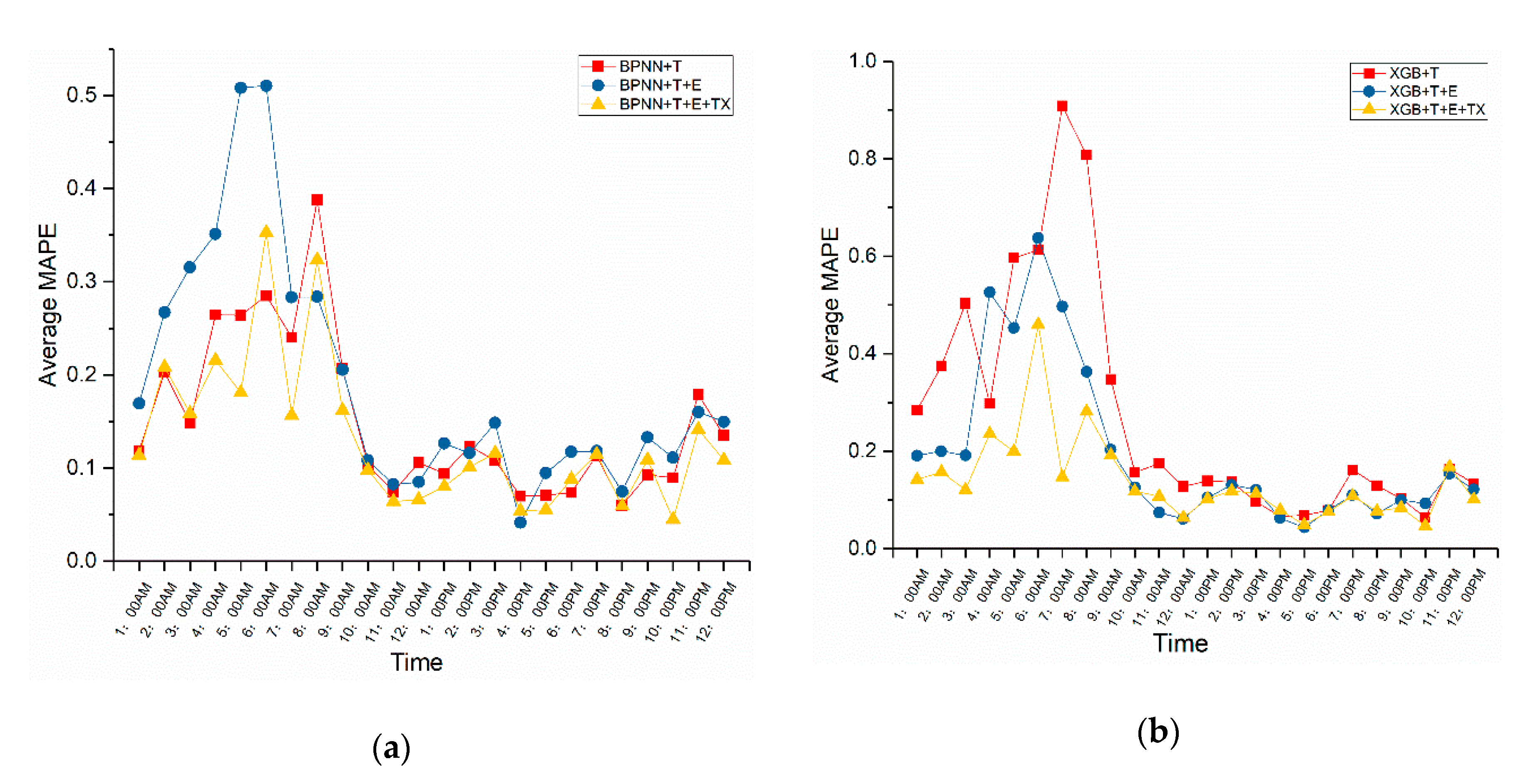
• Based on the BPNN methods, including information “E” leads to an MAPE reduction from 0.224 to 0.190 while it decreases RMSE from 28.576 to 23.921, and it increases the ${\mathrm{R}}^2$ from 0.819 to 0.845. Likewise, including information “TX” leads to an MAPE reduction from 0.190 to 0.132, and it increases the ${\mathrm{R}}^2$ from 0.845 to 0.866. Figure 7a shows that model “BPNN + T + E + TX” obtains the lowest MAPE among three predictions except at 6 a.m., 8 a.m. and 9 p.m., and from Figure 8, we know that model “BPNN + T + E + TX” obtains the lowest RMSE among three predictions except at 4, 7, and 9 p.m.;
• Based on the XGB methods, including information “E” leads to an MAPE reduction from 0.333 to 0.197 while it reduces RMSE from 26.296 to 21.206, and it increases the ${\mathrm{R}}^2$ from 0.833 to 0.857. And including information “TX” leads to an MAPE reduction from 0.197 to 0.139, and it increases the ${\mathrm{R}}^2$ from 0.857 to 0.865. Figure 7b indicates that the performance of the model “XGB + T + E + TX” is the best, except at 11 a.m. and 5 p.m., and from Figure 8 we know that performance of model “XGB + T + E + TX” is the best except at 11 a.m., 12 a.m., 4 p.m. and 5 p.m.;
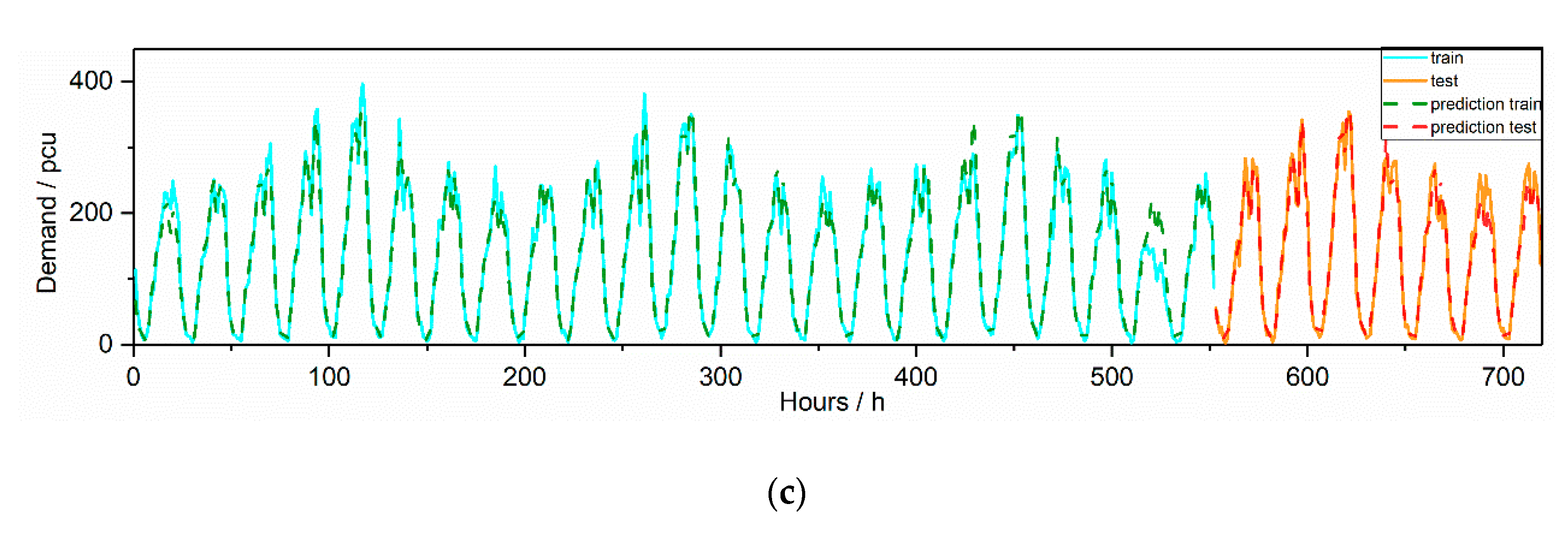
• We found that the model “BPNN + T + E + TX” is available for forecasting online taxi-hailing demand. The performance of the model, which includes information of “PTX”, is better than the model “BPNN + T + E”, but its accuracy is lower than the model “BPNN + T + E + TX”. Compared with the model “BPNN + T + E”, including the information of “PTX” leads to a reduction of MAPE from 0.190 to 0.183 and an RMSE reduction from 23.921 to 21.050, and it increases ${\mathrm{R}}^2$ from 0.845 to 0.853. This indicates that considering the information of “PTX” improves the predictability of online taxi-hailing demand. However, due to a reduction in the accuracy of “PTX”, the performance of the model “BPNN + T + E + TX” is better than the model “BPNN + T + E + PTX”.

However, the research still has some limitations. In the future, these limitations should be studied. For example, we did not use linear regression models to predict online taxi-hailing demand. Moreover, we should propose a method to forecast multiple trip demands simultaneously. Additionally, we will set projected environmental data as factors of real-time demand prediction for real-time forecasting.

6.2. Conclusions

In this research, the data-driven forecasting method of online taxi-hailing demand is carried out. To improve the prediction effects of online taxi-hailing demand, we proposed two methods for predicting online taxi-hailing demand based on BPNN and XGB, respectively. Then, we tested the two methods considering the information of “T”, “E” and “TX”. The results indicate that considering more information could improve the prediction accuracy of the models. Next, we forecasted the taxi demand and introduced a real-time online taxi-hailing demand forecasting method based on the projected taxi demand. We found that including the information of “PTX” improved prediction performance of model “BPNN + T + E”. Furthermore, MAPE, RMSE and ${\mathrm{R}}^2$ of the testing set of the model “BPNN + T + E + PTX” are, respectively, improved to 0.183, 21.050, and 0.853. Because the more precise traffic demand forecasting method can provide a more reasonable basis for public resources’ dispatch, the proposed method is cost-effective in the intelligent transportation system.

Furthermore, more experiments about traffic demand prediction can be considered. For instance, the multi-mode traffic demand predictor could be proposed to improve the prediction accuracy by considering the interaction among multiple modes of transportation. Meanwhile, the multi-mode traffic demand predictor can also take the interaction among different regions into account.

References

1. Chang, H.-W.; Tai, Y.-C.; Hsu, J.Y.-J. Context-aware taxi demand hotspots prediction. Int. J. Bus. Intell. Data Min. 2010, 5, 3–18. [Google Scholar] [CrossRef]
2. Moreira-Matias, L.; Gama, J.; Ferreira, M.; Damas, L. A predictive model for the passenger demand on a taxi network. In Proceedings of the 2012 15th International IEEE Conference on Intelligent Transportation Systems, Anchorage, AK, USA, 16–19 September 2012; pp. 1014–1019. [Google Scholar]
3. Moreira-Matias, L.; Gama, J.; Ferreira, M.; Mendes-Moreira, J.; Damas, L. On Predicting the Taxi-Passenger Demand: A Real-Time Approach. In Portuguese Conference on Artificial Intelligence; Springer: Berlin/Heidelberg, Germany, 2013; pp. 54–65. [Google Scholar]
4. Moreira-Matias, L.; Gama, J.; Ferreira, M.; Mendes-Moreira, J.; Damas, L. Predicting Taxi–Passenger Demand Using Streaming Data. IEEE Trans. Intell. Trans. Syst. 2013, 14, 1393–1402. [Google Scholar] [CrossRef] [Green Version]
5. Zhang, K.; Feng, Z.; Chen, S.; Huang, K.; Wang, G. A Framework for Passengers Demand Prediction and Recommendation. In Proceedings of the 2016 IEEE International Conference on Services Computing (SCC), San Francisco, CA, USA, 27 June–2 July 2016; pp. 340–347. [Google Scholar]
6. Jagannathan, N.D.G.R.K. A Multi-Level Clustering Approach for Forecasting Taxi Trip demand. In Proceedings of the IEEE 19th International Conference on Intelligent Transportation Systems (ITSC), Rio de Janeiro, Brazil, 1–4 November 2016; pp. 223–228. [Google Scholar]
7. Peng, X.; Pan, Y.; Luo, J. Predicting high taxi demand regions using social media check-ins. In Proceedings of the 2017 IEEE International Conference on Big Data (Big Data), Boston, MA, USA, 11–14 December 2017; pp. 2066–2075. [Google Scholar]
8. Zhao, K.; Khryashchev, D.; Freire, J.; Silva, C.; Vo, H. Predicting taxi demand at high spatial resolution: Approaching the limit of predictability. In Proceedings of the 2016 IEEE International Conference on Big Data (Big Data), Washington, DC, USA, 5–8 December 2016; pp. 833–842. [Google Scholar]
9. Xu, J.; Rahmatizadeh, R.; Boloni, L.; Turgut, D. A Sequence Learning Model with Recurrent Neural Networks for Taxi Demand Prediction. In Proceedings of the 2017 IEEE 42nd Conference on Local Computer Networks (LCN), Singapore, 9-12 October 2017; pp. 261–268. [Google Scholar]
10. Zhang, D.; He, T.; Lin, S.; Munir, S.; Stankovic, J.A. Taxi-Passenger-Demand Modeling Based on Big Data from a Roving Sensor Network. IEEE Trans. Big Data 2017, 3, 362–374. [Google Scholar] [CrossRef]
11. Bao, Y.; Sun, Y.-E.; Bu, X.; Du, Y.; Wu, X.; Huang, H.; Luo, Y.; Huang, L. How Do Metro Station Crowd Flows Influence the Taxi Demand Based on Deep Spatial-Temporal Network? In Proceedings of the 2018 14th International Conference on Mobile Ad-Hoc and Sensor Networks (MSN), Shenyang, China, 6–8 December 2018; pp. 188–192. [Google Scholar]
12. Davis, N.; Raina, G.; Jagannathan, K. Taxi Demand Forecasting: A HEDGE-Based Tessellation Strategy for Improved Accuracy. IEEE Trans. Intell. Transp. Syst. 2018, 19, 3686–3697. [Google Scholar] [CrossRef] [Green Version]
13. Markou, I.; Rodrigues, F.; Pereira, F.C. Real-Time Taxi Demand Prediction using data from the web. In Proceedings of the 2018 21st International Conference on Intelligent Transportation Systems (ITSC), Maui, HI, USA, 4–7 November 2018; pp. 1664–1671. [Google Scholar]
14. Ishiguro, S.; Kawasaki, S.; Fukazawa, Y. Taxi Demand Forecast Using Real-Time Population Generated from Cellular Networks. In Proceedings of the 2018 ACM International Joint Conference and 2018 International Symposium on Pervasive and Ubiquitous Computing and Wearable Computers—UbiComp ’18, Singapore, 8–12 October 2018; pp. 1024–1032. [Google Scholar]
15. Liao, S.; Zhou, L.; Di, X.; Yuan, B.; Xiong, J. Large-scale short-term urban taxi demand forecasting using deep learning. In Proceedings of the 2018 23rd Asia and South Pacific Design Automation Conference (ASP-DAC), Jeju, Korea, 22–25 January 2018; pp. 428–433. [Google Scholar]
16. Vanichrujee, U.; Horanont, T.; Pattara-Atikom, W.; Theeramunkong, T.; Shinozaki, T. Taxi Demand Prediction using Ensemble Model Based on RNNs and XGBOOST. In Proceedings of the 2018 International Conference on Embedded Systems and Intelligent Technology & International Conference on Information and Communication Technology for Embedded Systems (ICESIT-ICICTES), Khon Kaen, Thailand, 7–9 May 2018; pp. 1–6. [Google Scholar]
17. Xu, J.; Rahmatizadeh, R.; Boloni, L.; Turgut, D. Real-Time Prediction of Taxi Demand Using Recurrent Neural Networks. IEEE Trans. Intell. Transp. Syst. 2018, 19, 2572–2581. [Google Scholar] [CrossRef]
18. Yao, H.; Wu, F.; Ke, J.; Tang, X.; Jia, Y.; Lu, S.; Gong, P.; Ye, J.; Chuxing, D.; Li, Z. Deep Multi-View Spatial-Temporal Network for Taxi Demand Prediction. In Proceedings of the Thirty-Second AAAI Conference on Artificial Intelligence, New Orleans, LA, USA, 2–7 February 2018; pp. 2588–2595. [Google Scholar]
19. Zhang, W.; Ukkusuri, S.; Yang, C. Modeling the Taxi Drivers’ Customer-Searching Behaviors outside Downtown Areas. Sustainability 2018, 10, 3003. [Google Scholar] [CrossRef] [Green Version]
20. Yan, H.; Zhang, Z.; Zou, J. An online spatio-temporal model for inference and predictions of taxi demand. In Proceedings of the 2017 IEEE International Conference on Big Data (Big Data), Boston, MA, USA, 11–14 December 2017; pp. 3550–3557. [Google Scholar]
21. Kuang, L.; Yan, X.; Tan, X.; Li, S.; Yang, X. Predicting Taxi Demand Based on 3D Convolutional Neural Network and Multi-task Learning. Remote Sens. 2019, 11, 1265. [Google Scholar] [CrossRef] [Green Version]
22. Liu, L.; Qiu, Z.; Li, G.; Wang, Q.; Ouyang, W.; Lin, L. Contextualized Spatial–Temporal Network for Taxi Origin-Destination Demand Prediction. IEEE Trans. Intell. Transp. Syst. 2019, 20, 3875–3887. [Google Scholar] [CrossRef] [Green Version]
23. Markou, I.; Kaiser, K.; Pereira, F.C. Predicting taxi demand hotspots using automated Internet Search Queries. Transp. Res. Part C Emerg. Technol. 2019, 102, 73–86. [Google Scholar] [CrossRef]
24. Qiu, Z.; Liu, L.; Li, G.; Wang, Q.; Xiao, N.; Lin, L. Taxi Origin-Destination Demand Prediction with Contextualized Spatial-Temporal Network. In Proceedings of the 2019 IEEE International Conference on Multimedia and Expo (ICME), Shanghai, China, 8–12 July 2019; pp. 760–765. [Google Scholar]
25. Rodrigues, F.; Markou, I.; Pereira, F.C. Combining time-series and textual data for taxi demand prediction in event areas: A deep learning approach. Inf. Fusion 2019, 49, 120–129. [Google Scholar] [CrossRef] [Green Version]
26. Terroso-Saenz, F.; Munoz, A.; Cecilia, J.M. QUADRIVEN: A Framework for Qualitative Taxi Demand Prediction Based on Time-Variant Online Social Network Data Analysis. Sensors 2019, 19, 4882. [Google Scholar] [CrossRef] [PubMed] [Green Version]
27. Xu, Y.; Li, D. Incorporating Graph Attention and Recurrent Architectures for City-Wide Taxi Demand Prediction. ISPRS Int. J. Geo-Inf. 2019, 8, 414. [Google Scholar] [CrossRef] [Green Version]
28. Yu, H.; Chen, X.; Li, Z.; Zhang, G.; Liu, P.; Yang, J.; Yang, Y. Taxi-Based Mobility Demand Formulation and Prediction Using Conditional Generative Adversarial Network-Driven Learning Approaches. IEEE Trans. Intell. Transp. Syst. 2019, 20, 3888–3899. [Google Scholar] [CrossRef]
29. Liu, X.; Sun, L.; Sun, Q.; Gao, G. Spatial Variation of Taxi Demand Using GPS Trajectories and POI Data. J. Adv. Trans. 2020, 2020, 7621576. [Google Scholar] [CrossRef]
30. Saadallah, A.; Moreira-Matias, L.; Sousa, R.; Khiari, J.; Jenelius, E.; Gama, J. BRIGHT—Drift-Aware Demand Predictions for Taxi Networks. IEEE Trans. Knowl. Data Eng. 2020, 32, 234–245. [Google Scholar] [CrossRef]
31. Safikhani, A.; Kamga, C.; Mudigonda, S.; Faghih, S.S.; Moghimi, B. Spatio-temporal modeling of yellow taxi demands in New York City using generalized STAR models. Int. J. Forecast. 2020, 36, 1138–1148. [Google Scholar] [CrossRef] [Green Version]
32. Liu, Z.; Chen, H.; Li, Y.; Zhang, Q. Taxi Demand Prediction Based on a Combination Forecasting Model in Hotspots. J. Adv. Trans. 2020, 2020, 1302586. [Google Scholar] [CrossRef]
33. Wang, Z.; Luo, P.; Cheng, L.; Zhang, S.; Shen, J. Hapten-antibody recognition studies in competitive immunoassay of alpha-zearalanol analogs by computational chemistry and Pearson Correlation analysis. J. Mol. Recognit. 2011, 24, 815–823. [Google Scholar] [CrossRef]
34. Rajabi-Kiasari, S.; Hasanlou, M. An efficient model for the prediction of SMAP sea surface salinity using machine learning approaches in the Persian Gulf. Int. J. Remote Sens. 2020, 41, 3221–3242. [Google Scholar] [CrossRef]
35. Wang, J.-Z.; Wang, J.-J.; Zhang, Z.-G.; Guo, S.-P. Forecasting stock indices with back propagation neural network. Expert Syst. Appl. 2011, 38, 14346–14355. [Google Scholar] [CrossRef]
36. Selbesoglu, M.O. Spatial Interpolation of GNSS Troposphere Wet Delay by a Newly Designed Artificial Neural Network Model. Appl. Sci. 2019, 9, 4688. [Google Scholar] [CrossRef] [Green Version]
37. Karsoliya, S. Approximating Number of Hidden layer neurons in Multiple Hidden Layer BPNN Architecture. Int. J. Eng. Trends Technol. 2012, 3, 714–717. [Google Scholar]
38. Liu, Y.; Jiang, W.; Zhang, X. Research on Optimized Energy Scheduling of Rural Microgrid. Appl. Sci. 2019, 9, 4641. [Google Scholar] [CrossRef] [Green Version]
Figure 1. An instance of three-layer backpropagation neural network (BPNN).
Applsci 10 06681 g001
Figure 2. An instance of One-Hot Encoder.
Applsci 10 06681 g002
Figure 3. Research scope in the Bell Tower area.
Applsci 10 06681 g003
Figure 4. The demand for taxi and online taxi-hailing in Bell Tower area.
Applsci 10 06681 g004
Figure 5. Online taxi-hailing demand prediction results of models based on BPNN. (a) Result of model “BPNN + T”; (b) Result of model “BPNN + T + E”; (c) Result of model “BPNN + T + E + TX”.
Applsci 10 06681 g005aApplsci 10 06681 g005b
Figure 6. Online taxi-hailing demand prediction results of models based on extreme gradient boosting (XGB). (a) Result of model “BPNN + T”; (b) Result of model “BPNN + T + E”; (c) Result of model “BPNN + T + E + TX”.
Applsci 10 06681 g006aApplsci 10 06681 g006b
Figure 7. Average mean absolute percentage error (MAPE) of online taxi-hailing demand prediction based on BPNN and XGB in different hours. (a) MAPE of the prediction models based on BPNN; (b) MAPE of the prediction models based on XGB.
Applsci 10 06681 g007
Figure 8. Average RMSE of online taxi-hailing demand prediction based on BPNN and XGB in different hours. (a) RMSE of the prediction models based on BPNN; (b) RMSE of the prediction models based on XGB.
Applsci 10 06681 g008
Figure 9. The taxi demand prediction based on “BPNN + T + E” and “XGB + T + E”. (a) Result of taxi demand prediction based on “BPNN + T + E”; (b) Result of taxi demand prediction based on “XGB + T + E”.
Applsci 10 06681 g009
Figure 10. The demand prediction of online taxi-hailing based on the model “BPNN + T + E + PTX”.
Applsci 10 06681 g010
Figure 11. Prediction effects of online taxi-hailing demand predictions in different hours. (a) Average RMSE of online taxi-hailing demand predictions in different hours; (b) Average MAPE of online taxi-hailing demand predictions in different hours.
Applsci 10 06681 g011