1. Introduction
According to the assessment data of the American Cancer Society [
1], in 2020, the United States is expected to have 191,930 new cases of prostate cancer, and the number of deaths from prostate cancer will reach 33,330. Prostate cancer has surpassed lung cancer by turning out to be the most common due to the extensive increase of screening in 2016 [
2]. Accurate prostate gland segmentation and volume estimation play a vital role in the diagnosis and treatment of prostate-related diseases, especially the staging assessment of prostate cancer. At present, magnetic resonance imaging (MRI) has become the main imaging method for assisted prostate diagnosis due to its high-resolution and soft-tissue contrast [
3]. However, the examination of the prostate MRI scan is a slice-by-slice visual inspection performed by the radiologist, which is quite time-consuming, complicated, and subjective. Hence, in the past decade, various automatic prostate segmentation methods have been proposed.
For instance, Shi et al. [
4] exploited the coupled feature characterization and Spatial-Constrained Transductive LassO to estimate the 3D prostate likelihood map and used the multimap label fusion strategy to generate the final segmentation result. A deformable prostate segmentation method proposed by Guo et al. [
5] combined the deep feature learning model and sparse patch matching method to achieve prostate segmentation. These methods have actually shown an encouraging effect in the automatic segmentation of the prostate. However, due to the heterogeneity of the gland itself, the low contrast between the gland and surrounding tissues, and the lack of strong boundaries [
6], the segmentation of prostate remains a challenging task.
1.1. Deep-Learning Methods for 3D MR Image Segmentation
With the development of deep learning technology [
7,
8,
9,
10,
11], deep convolutional neural networks (CNNs) have been proven to be an effective tool for medical image analysis [
12,
13] and are increasingly used in segmentation tasks. The deep learning methods applied to 3D MRI segmentation can be roughly divided into the following three categories according to the data processing dimension.
1.1.1. Methods with 2D Manners
The first way treats each slice of the 3D MR images as a separate image and inputs it into the network to achieve pixel-wise segmentation. These methods, headed by FCN [
14] and U-Net [
15], are famous for their lightweight network architecture, so they are very suitable for medical image datasets with small-scale. For example, Tian et al. [
16] proposed a variant of FCN called PSNet, which used knowledge transfer from natural images to medical images to yield accurate segmentation of prostate MRI. Xiao et al. [
17] introduced a residual jump connection and weighted attention mechanism based on U-Net to realize the segmentation of blood vessels in retinal images. Similarly, Azad et al. [
18] designed a bidirectional convolution dense convolution U-Net (BCDU-Net) and achieved excellent performance in retinal vessel segmentation, skin lesion segmentation, and lung segmentation. All the above methods show that pixel-wise semantic segmentation has outstanding advantages in 2D fine-grained segmentation.
1.1.2. Methods with 3D Manners
The second way is to directly utilize 3D images as model input to achieve voxel-wise image segmentation. Milletari et al. [
19] extended U-net to 3D manners to perform volume segmentation of the prostate. Chen et al. [
20] proposed a new voxel residual network, which addressed the challenging problem of segmentation of key brain tissue in 3D MR images by introducing residual learning to volume data processing. Compared with 2D methods, 3D segmentation models can capture spatial context information better and usually have more parameters, which require sufficient training data to achieve reliable parameter adjustments. However, due to the anisotropy of 3D images, that is, when the interslice spacing is larger than the intraslice spacing, directly extending the 2D image segmentation method to 3D manners may not yield satisfactory performance. For instance, Baumgartner, C.F et al. [
21] compared the segmentation performance of modified 2D U-Net and 3D U-Net on the left ventricle, right ventricle, and myocardium on the ACDC 2017 challenge dataset. Experiments showed that the modified version of 2D U-Net outperformed the modified 3D U-Net.
1.1.3. Methods with 2D Sequence Manners
The third method converts 3D MR images into 2D sequence images as model input. This type of method comprehensively takes into account the defects of 2D and 3D manners. Based on 2D segmentation, it produces more accurate results by learning the interslice correlation and consistency. Chen et al. [
22] proposed the comprehensive use of FCN and recurrent neural network (RNN) to mine the intraslice and interslice context information in 3D images, respectively, and realized the neuron structure segmentation in 3D EM images and 3D fungal segmentation. To improve the prostate segmentation effect, Zhu et al. [
23] introduced a bidirectional convolutional LSTM block to build a U-shaped network and used subsequences composed of three consecutive slices as input to train the network. These methods showed encouraging performance for datasets with dense interslice correlation information. However, for 3D images with greater slice thickness or interslice spacing, the segmentation effect needs to be further explored.
1.2. Cascaded Multistage Methods for Medical Image Segmentation
At present, the two mainstream segmentation modes of deep learning methods in the field of image segmentation include end-to-end segmentation and cascade segmentation. End-to-end segmentation uses only a single model to directly implement the segmentation task, while cascaded segmentation refers to the use of multistage processing to achieve stepwise segmentation. In contrast, end-to-end segmentation better avoids the accumulation of errors in multistage segmentation and simplifies the segmentation process. However, the high integration of a single model leads to its poor flexibility, operability, and interpretability. At the same time, a single model may need more training data to achieve better results. Therefore, there are still many researchers who employ cascade methods in medical image segmentation [
24,
25,
26]. Xie et al. [
24] proposed a cascaded SE-ResNeXT U-Net for kidney tumor segmentation. In the wrist reference bone segmentation, Chen et al. [
25] first utilized the target detection algorithm to extract the region of interest and then achieved the reference bone segmentation using the segmentation network.
1.3. Attention Mechanism in Image Analysis Tasks
The attention mechanism was first applied in machine translation, and its applications in computer vision tasks such as target detection and image segmentation are gradually increasing [
27,
28,
29,
30,
31]. The combination of this visual attention mechanism and deep learning has gradually evolved into two types of attention—hard attention and soft attention. Hard attention, such as spatial pooling and image cropping, is not differentiable, which emphasizes areas that need attention. Elsayed et al. [
29] proposed a hard-attention model named Saccader, achieving good classification accuracy on ImageNet while only covering part of the image. In contrast, soft attention, as a probability distribution map between [0, 1], emphasizes the degree of attention of each area, and it can update the weight through the back propagation of the neural network. Jaderberg et al. [
30] designed a spatial transformer model to focus on key spatial domain information. Woo et al. [
31] constructed a convenient and lightweight mixed-domain attention module on the channel and space, achieving classification performance improvements on multiple benchmark architectures.
1.4. Contributions
Some of the above algorithms have achieved promising performance in prostate MR segmentation. Notwithstanding, in terms of prostate images with fuzzy or even missing edge information, as well as images at both ends of the sequence with small gland proportions and weak edge features, prostate segmentation is still a challenge. In addition, exploiting the limited dataset more effectively to improve the segmentation performance is also a problem worth exploring.
To this end, this paper proposes a cascaded dual attention network (CDA-Net) for prostate MR segmentation. The algorithm adopts a cascade segmentation method, including two stages of ROI extraction and fine segmentation. Firstly, the improved Faster R-CNN with sequence correlation postprocessing (named RAS-FasterRCNN) is utilized to perform preliminary localization of the prostate. Secondly, an encoder-decoder architecture (called RAU-Net) that integrates residual learning and soft attention mechanism is used to achieve precise segmentation of the prostate. The algorithm was evaluated on two public databases, presenting excellent segmentation accuracy and generalization performance.
The main contributions of this work can be summarized as follows:
(1) The algorithm uses a cascaded dual attention mechanism to progressively advance the extraction of the precise contours of the prostate organs. Firstly, bounding box regression adjustment is applied to achieve ROI extraction. This hard attention mechanism excludes the influence of adjacent tissues around the prostate and other redundant background information well. Secondly, a trainable soft attention gate mechanism is introduced in the subsequent segmentation network. It dynamically learns the implicit attention distribution in the feature maps to enable the network to focus on the organ areas, thereby improving the accuracy of segmentation. Compared with the single-stage end-to-end segmentation method, this algorithm is more robust and flexible.
(2) The algorithm combines the advantages of segmentation methods in 2D and 3D manners. The application of 2D segmentation allows the network to be fully trained under small-scale datasets. Meanwhile, in view of the weak interslice correlation and consistency of organ positions, the algorithm adds the spatial curve fitting strategy in the sequence direction in the ROI extraction phase, which significantly improves the initial localization effect, establishing a good foundation for subsequent segmentation.
The rest of this paper is organized as follows: in
Section 2, the source of the datasets and data augmentation methods are described.
Section 3 details the entire framework of the algorithm. Qualitative and quantitative experimental results obtained on two public datasets are shown in
Section 4.
Section 5 presents conclusions about the contributions and segmentation performance as well as directions for future research.
2. Materials
Two public datasets were used in this study. They are the PROMISE12 dataset published in the MICCAI2012 Prostate Segmentation Challenge [
6] and the ASPS13 dataset published in the ISBI2013 Prostate Structure Segmentation Challenge [
32].
2.1. The PROMISE12 Dataset
The PROMISE12 dataset comes from four different medical centers, and it includes both patients with benign disease (e.g., benign prostatic hyperplasia) and prostate cancer. It contains 80 available T2-weighted axial MR images of the prostate, 50 of which have expert segmentation masks while the remaining 30 do not. The in-plane image size varies from 256 × 256 to 512 × 512 pixels. In MRI images, the pixel/voxel intensities and appearance characteristics of the prostate can significantly depend on different acquisition protocols and scanners.
Table 1 lists the details of the dataset, and
Figure 1 shows one sample scan from each center.
2.2. The ASPS13 Dataset
The ASPS13 dataset contains 80 T2-weighted MR images, together with the corresponding segmentation ground truth annotated by experts. All images collected in this dataset are from prostate cancer patients. Half of them were obtained at 1.5 T Philips Achieva with an ERC from Boston Medical Center (BMC), and the other half were obtained at 3 T Siemens TIM with a surface coil (SC) from Radboud University Nijmegen Medical Center (RUNMC). They were acquired as T2-weighted MR axial pulse sequences with either 4 mm thick slices at 3 T or 3 mm thick at 1.5 T. Given that this dataset has 11 overlapped subjects with PROMISE12, we removed them in the experiment and only kept the remaining 69 samples.
Figure 2 shows one scan from each center.
2.3. Data Augmentation
In this paper, to enable the network to get adequate training and parameter adjustment, before the network training, data augmentation approaches such as small random rotation, random translation (along the x and y directions), horizontal or vertical flip, and elastic deformation were performed on the training set images [
33]. In addition, 5% of Gaussian noise was randomly added during data enhancement to improve the anti-noise ability of the algorithm.
3. Methods
The algorithm proposed in this paper includes the following two steps: ROI extraction based on the RAS-FasterRCNN (i.e., the initial localization of the prostate) and fine segmentation based on the RAU-Net. The overall flowchart is shown in
Figure 3.
3.1. RAS-Faster RCNN for ROI Extraction
3.1.1. RA-FasterRCNN
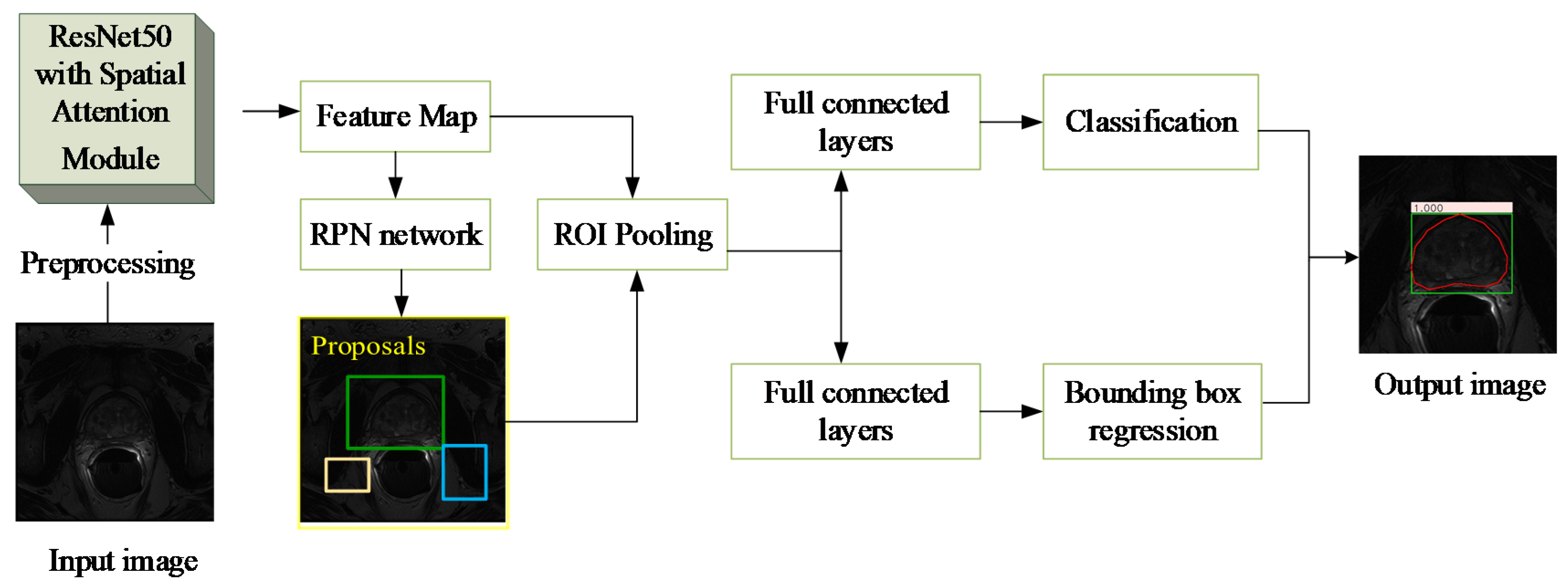
Generally, the area of the prostate organs is relatively small in the original image, especially for the apex and base parts of the prostate. Therefore, to eliminate the interference with the adjacent tissues and various artifacts as much as possible, while ensuring the integrity of the organ area, this paper adopted the improved Faster R-CNN [
34,
35,
36,
37] based on the residual network and the spatial attention mechanism (RA-FasterRCNN) to develop initial localization of the organ.
Figure 4 shows the main flow of the network, which mainly includes two parts: region extraction network (RPN) and object detection network (Fast R-CNN) [
38].
This algorithm first performs pixel intensity normalization and size normalization on each 2D axial scan in the 3D MR image. Then, each of the 2D slices is inputted into the RA-FasterRCNN to obtain a collection of prostate region proposals with high predicted probability and accurate locations. Compared with the original Faster RCNN, we used ResNet50 with spatial attention modules, which is described in detail in
Figure 5, instead of the original VGG16 as the feature extraction part of the network.
Besides, the function of the spatial attention module is shown in Equation (1), in which
represents the input feature map,
denote the global average pooling and global maximum pooling of
along the channel axis, respectively,
represents a convolution operation with a
convolution kernel,
is the Sigmoid function, [ ] means the splicing operation of two feature maps.
Considering the two tasks of bounding box classification and regression prediction, the training loss function is defined in Equation (2). Among them,
and
represent the binary cross-entropy loss and smoothL1 regression loss, respectively [
39],
is a weight coefficient between classification loss and regression loss.
It is worth noting that the trainable parameters in Resnet-50 in the network are pretrained on the ImageNet dataset [
40]. The transfer learning from natural images to medical images is often used to improve the small-scale defects of prostate image datasets [
41,
42].
3.1.2. Sequence Correlation Processing
Since Faster R-CNN was initially applied to object detection tasks in natural images, in the detection results of RA-FasterRCNN, multiple objects or lack of objects appeared in individual slice images (
Figure 4a,b). However, this situation should not exist for the task of prostate localization. Thus, this paper utilizes the uniqueness of the organ and the slight variation of the organ position in the same sequence of images and introduces sequence correlation processing to improve organ localization. Taking a sequence of MR images as an example, the detailed description is the following three steps:
Step 1: The object proposals with the credibility of RA-FasterRCNN detection results greater than a certain threshold are retained. In this paper, the threshold is set as 0.80 after repeated experiments.
Step 2: For the multi-box phenomenon shown in
Figure 6a: first, we take advantage of the uniqueness of the organ and the slight variation of the organ position in the sequence images to firstly select the slice images which have a single reliable organ bounding box in the sequence images. Nine key points (including the four vertices, the midpoint of each boundary and the center point of the organ proposal) of these slices are utilized for spatial curve fitting based on sequence direction. The fitting method is the least-square polynomial fitting. Then, the fitted spatial curves and the minimum spatial Euclidean Distance are applied to screen and determine the object bounding boxes closest to the fitted position in the slice images with multiple prediction boxes as the final position of the organ.
Figure 7 is a schematic diagram illustrating the above process. And Equation (3) describes the mathematical formula basis for screening. It is worth noting that the spatial curve parameters are updated after each screening.
where
indicates the final organ bounding box selected in a slice image,
and
denote the fitting prediction values of the
y-axis and
z-axis at the
key point,
and
represent the coordinate values of the
key point of the object box
predicted by the network on the
y-axis and
z-axis.
Step 3: For the missing object phenomenon, as shown in
Figure 6b: the final updated spatial curve is used to fit the organ position in the missing detection images.
3.1.3. Postprocessing
To ensure the spatial consistency of the sequence image in the subsequent segmentation, the final ROIs obtained by RAS-FasterRCNN are cropped in a uniform size according to the sequence unit and normalized to 256 × 256. The part of the cropped area beyond the ROI area is blacked out, meaning the background area. Afterward, for each 2D MR scan, pixel intensity normalization, contrast limited adaptive histogram equalization (CLAHE) [
43], and curvature driven image smoothing are implemented.
3.2. RAU-Net for Prostate Segmentation
3.2.1. The Architecture of RAU-Net
Recently, U-Net has become the backbone for many medical image segmentation tasks due to its ingenious U-shaped architecture and its low data demand [
9,
18,
19,
23,
24,
44]. The network consists of encoding and decoding paths. The encoder performs feature extraction and captures context information through a series of convolution and downsampling operations. The decoder is gradually restored to the original image size through upsampling to produce segmentation maps. Besides, the short connection between the codec parts enables the feature maps of the decoder to incorporate more low-level features, thereby increasing the segmentation accuracy of the model.
At present, the variant ideas of the network are mainly concentrated in two aspects. The first is how to better use the image features of different levels in the encoding and decoding stage, such as introducing the idea of dense connections or residual connections. The second is how to establish a better connection between the encoding and decoding stages to achieve better information fusion.
This paper draws on the above two ideas. We introduce the residual mechanism and soft attention mechanism to build an encoder-decoder architecture to achieve fine segmentation of the prostate organs. The architecture diagram of the network is shown in
Figure 8.
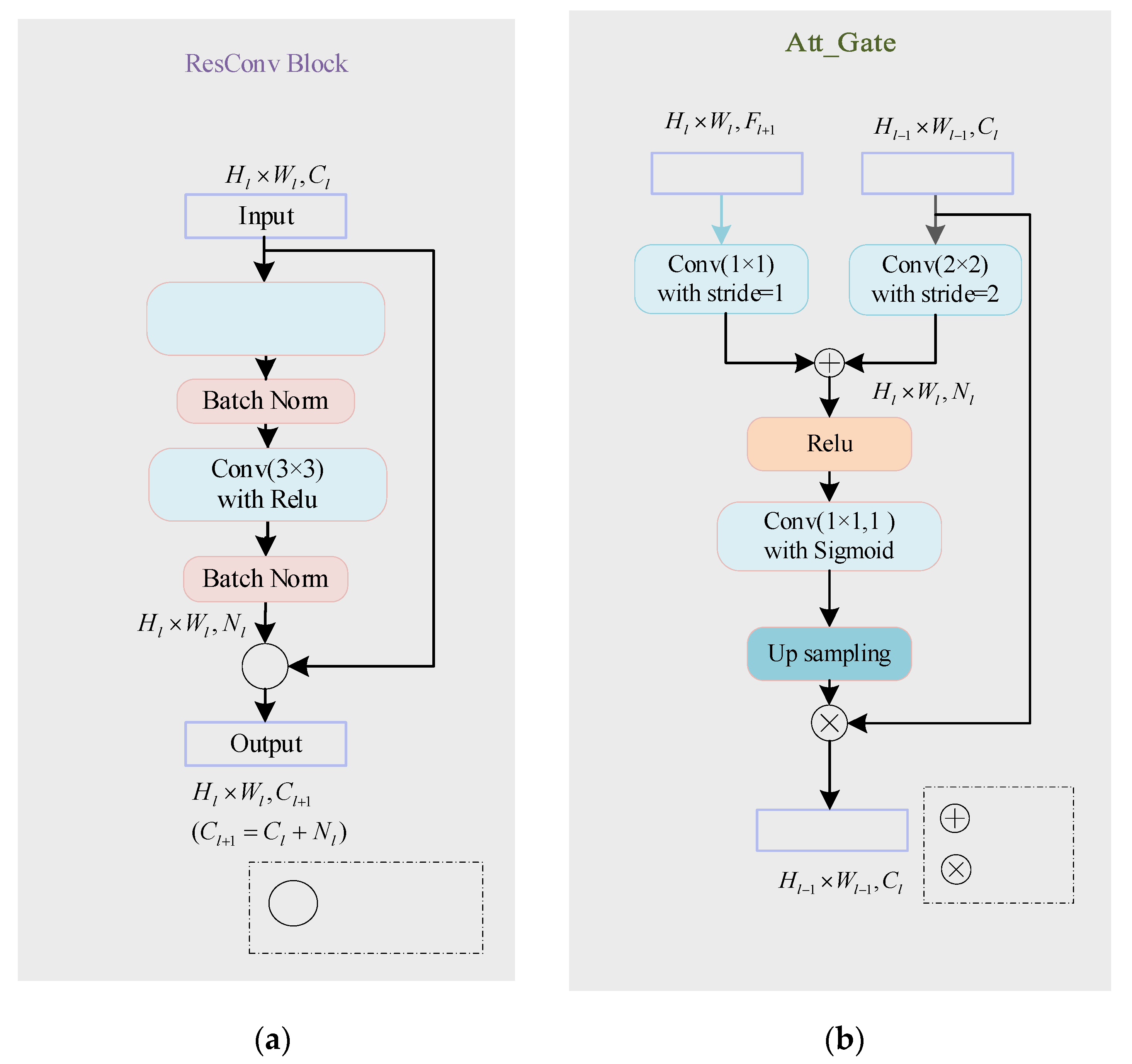
The network inputs a 2D image to be segmented and outputs a probability prediction map of the same size as the input image. In order to better improve the network’s utilization of features at different levels and ensure the network’s training convergence during the network deepening process, this paper introduces ResConv Block before downsampling and upsampling operations in the encoding and decoding stages. It consists of two Conv/BN blocks (as shown in
Figure 9a). The BatchNormalization layer improves the gradient dispersion by normalizing the convolution output and speeds up the network convergence [
45]. The encoding stage is composed of seven sub-blocks, which comprise ResConv Block and Max pooling. Each time the input feature map passes through the ResConv Block, the number of channels is doubled (i.e.,
), and the image size halved after each Max pooling (i.e.,
). As the number of downsampling increases, the receptive field of feature extraction gradually increases. Therefore, the network’s grasp of image details and features gradually weakens, and the grasp of image deep semantic information gradually increases. Symmetrically, the decoding stage consists of seven sub-blocks, which are composed of ResConv Block and upsampling. Each time the input passes through the ResConv Block, the number of channels is halved, and the image size is doubled after each pass through upsampling.
3.2.2. Self-Attention Gating Mechanism
To improve the accuracy of network segmentation and better integrate the deep semantic features and shallow detail features, this paper introduces a self-attention gating module before the splicing operation similar to U-Net. As shown in
Figure 9b, taking
,
as input and
as output, the attention gating module
can be formulated as:
where
and
denote the ReLU function and Sigmoid function, respectively.
in the decoding path is added to the low-level feature map to generate the attention weight map. The weight map is multiplied by to achieve the activation of different degrees of importance to different regions in . As the feature map in the decoding stage integrates more image semantic information and contextual information, the soft region suggestion generated implicitly in combination with it is closely related to the segmentation task. The attention distribution acts as a gating signal on the shallow feature map generated in the encoding stage, which can filter out the noise information of the background area in the low-level features that are not related to the segmentation task, reduce the feature activation of the background area, and achieve more efficient fusion of encoding and decoding features to improve the accuracy of label prediction.
3.2.3. The Objective Function
The loss function chosen in this paper is based on the Dice Similarity Coefficient (DSC). Compared with the binary cross-entropy loss function, this loss function can pay more attention to the segmentation of the foreground area, and can better deal with the problem of category imbalance. In recent years, it has gradually been widely used in many medical image segmentation competitions and papers [
20,
23,
46,
47,
48]. The DSC function is usually used to measure the overlap rate between the predicted segmentation and the ground truth, as shown in Equation (5).
in which
and
represent predicted mask and the ground truth, respectively.
Since a higher DSC index means better segmentation performance, we hope that the training loss function value can converge to a minimum. Furthermore, the ground truth in this paper is a binary image, and the prediction segmentation is a probability map. Therefore, the training loss function is defined as:
where
represents the total number of pixels in the image, and
, respectively, indicate the probability that pixel
from predicted segmentation and ground truth belongs to the foreground organ.
4. Experiments and Discussion
4.1. Implementation Details
In our experiments, the training and inference of the proposed algorithm CDA-Net were implemented in Tensorflow and Keras with Tensorflow backend. Additionally, all the experiments ran on a PC with Intel® Core™ i7 3.00 GHz processors, 32 GB of RAM, and 1 NVIDIA GeForce RTX 2080 SUPER Graphics Processing Unit (GPU).
The model training in our algorithm used Adam [
49] optimizer with default parameters
,
,
. Among them, the initial learning rate of RAS-FasterRCNN is set as 0.1, and the iteration is 70 times. The initial learning rate of the RAU-Net model is set to 0.1, and the iteration is 50 times. The total training time of the two networks is about 12 h. The average processing time of each test slice image is approximately 0.4 s.
4.2. Experiment Setting and Evaluations
This paper conducted a series of quantitative and qualitative comparison experiments to evaluate the effectiveness of the CDA-Net. In this paper, 50 cases with ground truths in PROMISE12 were randomly divided into a training set and a test set according to the ratio of 4:1. The remaining 30 samples without annotations (referred to as Test30) were applied to the visual evaluation of the algorithm generalization performance. In addition, all 69 cases in the ASPS13 dataset were used as test sets and did not participate in model training. The intermediate results of the algorithm during the testing of the two data sets are shown in
Figure A1, which also shows the improvement of the localization effect before and after the sequence correlation processing.
4.2.1. Quantitative Comparison with State-of-the-Art Algorithms
We compared the results of our CDA-Net against several other algorithms, which have also been applied to the PRIMOSE12 dataset. Since most methods do not give open source implementation code, we directly used the test results given by these algorithms except the FCN and U-Net. The comparison results are listed in
Table 2. Due to the inconsistent evaluation mechanisms adopted by different approaches, we utilized the most commonly used DSC in the field of medical image segmentation to compare the segmentation effects. The comparison results indicate that the value of DSC of our algorithm on the PROMISE12 dataset is significantly higher than other popular algorithms, which means that the predicted segmentation result of our algorithm is closest to the real segmentation mask.
4.2.2. Ablation Experiments
In this paper, two ablation experiments were conducted on the PROMISE12 test sets and ASPS13 dataset. In order to fully guarantee the effectiveness of the comparison experiment, the U-Net-1 here maintained the same basic architecture parameters as the algorithm RAU-Net in this paper. Based on U-Net [
15], the initial network channel number is set to 8, and the downsampling and upsampling depths are both 7. ResU-Net and RAU-Net also use U-Net-1 as the benchmark, and successively add residual convolution blocks and attention gate mechanism. At the same time, the four algorithms are consistent in dataset allocation, image preprocessing, and data augmentation operations.
The segmentation effects were assessed by five criteria—DSC, relative volume difference (RVD), segmentation accuracy (SA), oversegmentation rate (OR), undersegmentation rate (UR).
RVD measures the difference between the predicted segmentation volume X and the real segmentation volume Y.
SA, which is equivalent to the segmentation recall rate, is calculated as the ratio of correct prediction of pixels in the real foreground area by the algorithm.
OR represents the oversegmentation rate of the algorithm, which can be described as follows:
UR reflects the undersegmentation rate of the algorithm, that is
where TP, FP, TN, and FN denote the number of true positives, false positives, true negatives, and false negatives.
Experiment 1. Ablation Experiments on the test set of PROMISE12
Table 3 lists the segmentation comparison results of the above four algorithms in the PROMISE12 test set. It can be seen that,
Compared with U-Net [
12], U-Net-1 and ResU-Net have a significant improvement in the value of DSC, which shows that the network’s mining of image deep features and full use of features at different levels does improve the effect of the predicted segmentation;
Besides, the addition of the attention gate mechanism in RAU-Net forces the network to pay more attention to real organ regions, therefore it shows more obvious advantages than the previous two algorithms in the results of multiple metrics, especially RVD and SA;
Finally, although the CDA-Net proposed in this paper is slightly worse in the OR and RVD, it increases by 2.71% and 4.72% in the DSC and SA compared to the RAU-Net. It indicates that although the algorithm may have a slight oversegmentation phenomenon, the recall rate for the real organ area and the prediction accuracy for the organ area is higher. This is closely related to the ROI patch extraction based on bounding box regression prediction performed by the algorithm before organ segmentation. Therefore, it also fully illustrates that the segmentation idea of using a cascaded dual attention mechanism is also worthy of respect.
In addition, in order to further intuitively present the segmentation performance of the algorithm, we visually displayed and compared the predicted segmentation and ground truth of the above four algorithms. The comparison results are shown in
Figure 10, where the red line marks the actual contour of the organ, the yellow line marks the outline of the predicted segmentation result obtained by the algorithms, and the fourth row is the segmentation result after ROI cropping.
Since slice images with high imaging quality and clear organ contours have almost achieved perfect segmentation performance in many segmentation algorithms, especially those based on deep learning, this paper does not involve much of such images. As shown in
Figure 10,
The first column compares the segmentation performance of each algorithm in the images with endorectal coils. It can be seen that the four algorithms based on the U-Net architecture are not excessively affected by coil artifacts and image contrast, and they have achieved relatively good performance;
The second column shows the performance of the four algorithms when the gray distribution inside the gland is obviously uneven. We can see that the predicted segmentation results of the U-Net-1 and ResU-Net algorithms are affected to varying degrees at this time. In contrast, the contours obtained by the RAU-Net and CDA-Net proposed in this paper can still have a good matching effect with the real segmentation contour, which fully reveals that the attention gate mechanism added in this paper can have a more accurate estimation of attention to the region where the organ is located, thereby guiding the algorithm to obtain a more reasonable segmentation result;
Besides, columns 3–5 specifically compare the segmentation performance of the algorithm on the apex and base of the slice sequences. It can be observed that the proportion of organs in the slice images at both ends of the organ is very small, and the contours of the organs in the base slices are often blurred. Therefore, this is usually the most challenging part of prostate segmentation, and it is also the key part that can distinguish the performance of the algorithm. Comparing the segmentation results of the four algorithms in the third and fourth columns, we can see that the algorithms ResU-Net and RAU-Net can better obtain the position of the organs than U-Net-1, but the accurate segmentation of the organs is still inferior to CDA-Net;
Similarly, in the fifth column, even though the organs are relatively small and the contours are irregular, the algorithm CDA-Net in this paper still achieves a better segmentation performance than the first three algorithms. It demonstrates that the initial ROI extraction based on the sequence correlation used in this paper can effectively locate the organ position, thereby greatly reducing the focus of subsequent fine segmentation, and making the CDA-Net algorithm present more significant advantages in the segmentation of prostate base and apex.
Experiment 2. Ablation Experiments on ASPS13
Table 4 lists the average results of the above four algorithms tested on the ASPS13 dataset. It can be seen that because the ASPS13 dataset is relatively less complex than the PROMISE12 dataset, it shows a more excellent segmentation performance in the ResU-Net and RAU-Net algorithms without ROI extraction. In addition, the segmentation results gap between RAU-Net and ResU-Net and between ResU-Net and U-Net-1 is obviously widened. This shows that in the case of relatively low image complexity, the residual convolution block and soft-attention mechanism introduced in RAU-Net can better mine the generalized features of the image, thereby better improving the pixel prediction effect. Through the comparison of
Table 3 and
Table 4, the ROI extraction proposed in CDA-Net has a more prominent effect on the final segmentation in organ segmentation with higher image complexity. However, in any case, the test results of CDA-Net on the two datasets showed the best performance.
4.2.3. Qualitative Evaluation
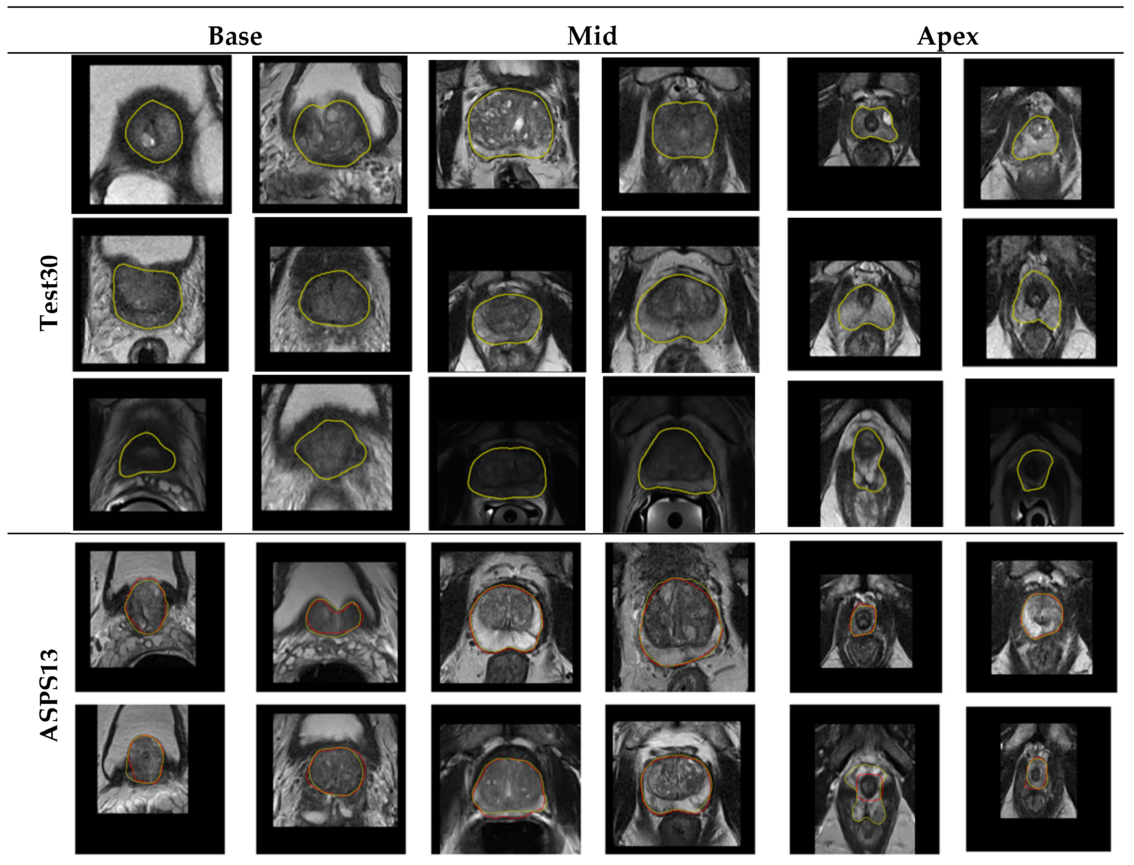
Figure 11 shows the segmentation performance of our algorithm in Test30 of PROMISE12 and ASPS13. It displays that the algorithm we proposed can overcome the low contrast of the image, the serious uneven distribution of the gray gradient inside the gland, and the poor gray contrast between the gland and surrounding tissues in the segmentation results of the central organ slices. In addition, in the slice image segmentation at both ends of the sequence, although some slices still have over- or undersegmentation, the contour extraction results of the algorithm can also match the ground truth to a large extent. All of the above illustrates the promising performance of the algorithm in organ segmentation at both ends of the sequence and the strong generalization ability of the whole algorithm.
5. Conclusions
Reliable prostate contour segmentation is essential for radiotherapy planning for prostate cancer. In order to improve the time-consuming problem of slice-by-slice visual inspection by traditional radiologists and the inter- and intraobserver difference, this paper presents a cascaded dual attention network CDA-Net for the fully automatic segmentation of prostate MR images. Taking the flexibility and robustness of the stage-wise segmentation algorithm into account, we firstly used the RAS-FasterRCNN method to realize the organ localization of the 2D slice image, and secondly employed the RAU-Net method to further realize the accurate segmentation of the prostate organ based on the ROI extraction.
(1) Due to the anisotropy of the prostate image, that is, the layer spacing between the axial slices is large, taking advantage of the weak correlation between the slices, this paper introduces sequence correlation processing based on spatial curve fitting to the back end of RA-FasterRCNN to improve poorly detected images. After the correlation processing, the success rate of organ localization on PROMISE12 and ASPS13 test sets reached 99.78% and 99.88%, respectively.
(2) In addition, we introduced residual connections based on U-Net to fuse the shallow and deep features of different levels. Channel splicing based on the attention gating mechanism is also added to highlight the network’s attention to the foreground organ area, suppress the feature activation of the background area and noise points, and effectively improve the pixel-level prediction accuracy of the network.
The experimental results show that exploiting only 40 training samples, the CDA-Net proposed in this paper achieved a mean dice score of 92.88% and 92.65% on the PROMISE12 test set with high heterogeneity and the ASPS13 dataset with larger scale. Similarly, in the visualization experiment, the algorithm has significantly improved the prediction effect of organ segmentation for difficult images such as obvious uneven gray distribution inside glands and blurred organ boundaries, especially for slice images at both ends of the sequence. It can be concluded that the advantages of the step-by-step attention focusing mechanism introduced by the algorithm are indeed convincing.
In future work, we will further improve the loss function settings of the segmentation algorithm, such as introducing boundary-based loss functions or cross-entropy loss function or combined loss functions, hoping to further improve the algorithm’s prediction effect on gland contours.
Author Contributions
Conceptualization, Z.L. and M.Z.; methodology, M.Z.; software, M.Z.; validation, M.Z. and Y.P.; formal analysis, Z.L. and M.Z.; investigation, Z.L., M.Z. and Y.P.; resources, Z.L.; data curation, M.Z.; writing—original draft preparation, M.Z.; writing—review and editing, Z.L. and Y.P.; visualization, M.Z.; supervision, Z.L.; project administration, Z.L. and Y.P.; funding acquisition, Z.L. All authors have read and agreed to the published version of the manuscript.
Funding
This research was supported by the National Natural Science Foundation of China under Grant 51677123.
Acknowledgments
We appreciate the organizers of the 2012 prostate MR image segmentation challenge for sharing the data set and opening up various method rankings and test results. At the same time, we are grateful to the organizers of the 2013 Prostate Structure Segmentation Challenge for their efforts in collecting and sharing data sets.
Conflicts of Interest
The authors declare that there is no conflict of interest regarding the publication of this paper.
Appendix A
Figure A1.
The intermediate results of CDA-Net during the testing of the two data sets
Figure A1.
The intermediate results of CDA-Net during the testing of the two data sets
References
- Siegel, R.L.; Mph, K.D.M.; Jemal, A. Cancer statistics, 2020. CA: Cancer J. Clin. 2020, 70, 7–30. [Google Scholar] [CrossRef] [PubMed]
- Mohler, J.L.; Armstrong, A.J.; Bahnson, R.R.; D’Amico, A.V.; Davis, B.J.; Eastham, J.A.; Enke, C.A.; Farrington, T.A.; Higano, C.S.; Horwitz, E.M.; et al. Prostate Cancer, Version 1.2016. J. Natl. Compr. Cancer Netw. 2016, 14, 19–30. [Google Scholar] [CrossRef] [PubMed]
- Leake, J.L.; Hardman, R.L.; Ojili, V.; Thompson, I.; Shanbhogue, A.; Hernández, J.; Barentsz, J. Prostate MRI: Access to and current practice of prostate MRI in the United States. J. Am. Coll. Radiol. 2014, 11, 156–160. [Google Scholar] [CrossRef] [PubMed]
- Shi, Y.; Gao, Y.; Liao, S.; Zhang, D.; Gao, Y.; Shen, D. Semi-Automatic Segmentation of Prostate in CT Images via Coupled Feature Representation and Spatial-Constrained Transductive Lasso. IEEE Trans. Pattern Anal. Mach. Intell. 2015, 37, 2286–2303. [Google Scholar] [CrossRef] [PubMed]
- Guo, Y.; Gao, Y.; Shen, D. Deformable MR Prostate Segmentation via Deep Feature Learning and Sparse Patch Matching. IEEE Trans. Med. Imaging 2015, 35, 1077–1089. [Google Scholar] [CrossRef]
- Litjens, G.; Toth, R.; Van De Ven, W.; Hoeks, C.; Kerkstra, S.; Van Ginneken, B.; Vincent, G.; Guillard, G.; Birbeck, N.; Zhang, J.; et al. Evaluation of prostate segmentation algorithms for MRI: The PROMISE12 challenge. Med. Image Anal. 2014, 18, 359–373. [Google Scholar] [CrossRef]
- Koirala, A.; Walsh, K.B.; Wang, Z.; McCarthy, C. Deep learning for real-time fruit detection and orchard fruit load estimation: Benchmarking of ‘MangoYOLO’. Precis. Agric. 2019, 20, 1107–1135. [Google Scholar] [CrossRef]
- Ma, C.; Huang, J.-B.; Yang, X.; Yang, M.-H. Robust Visual Tracking via Hierarchical Convolutional Features. IEEE Trans. Pattern Anal. Mach. Intell. 2018, 41, 2709–2723. [Google Scholar] [CrossRef]
- Li, X.; Chen, H.; Qi, X.; Dou, Q.; Fu, C.-W.; Heng, P. H-DenseUNet: Hybrid Densely Connected UNet for Liver and Tumor Segmentation from CT Volumes. IEEE Trans. Med. Imaging 2018, 37, 2663–2674. [Google Scholar] [CrossRef]
- Deng, Z.; Sun, H.; Zhou, S.; Zhao, J.; Lei, L.; Zou, H. Multi-scale object detection in remote sensing imagery with convolutional neural networks. ISPRS J. Photogramm. Remote Sens. 2018, 145, 3–22. [Google Scholar] [CrossRef]
- Chen, K.; Wang, P.; Yang, X.; Zhang, N.; Wang, D. A Model Output Deep Learning Method for Grid Temperature Forecasts in Tianjin Area. Appl. Sci. 2020, 10, 5808. [Google Scholar] [CrossRef]
- Lo, C.-M.; Chen, Y.-C.; Weng, R.-C.; Hsieh, K.L.-C. Intelligent Glioma Grading Based on Deep Transfer Learning of MRI Radiomic Features. Appl. Sci. 2019, 9, 4926. [Google Scholar] [CrossRef]
- Jiang, Y.; Wang, F.; Gao, J.; Cao, S. Multi-Path Recurrent U-Net Segmentation of Retinal Fundus Image. Appl. Sci. 2020, 10, 3777. [Google Scholar] [CrossRef]
- Long, J.; Shelhamer, E.; Darrell, T. Fully convolutional networks for semantic segmentation. In Proceedings of the IEEE Conference on Computer Vision and Pattern Recognition, Boston, MA, USA, 7–12 June 2015; pp. 3431–3440. [Google Scholar]
- Ronneberger, O.; Fischer, P.; Brox, T. U-net: Convolutional networks for biomedical image segmentation. In International Conference on Medical Image Computing and Computer-Assisted Intervention; Springer: New York, NY, USA, 2015; pp. 234–241. [Google Scholar]
- Tian, Z.; Liu, L.; Zhang, Z.; Fei, B. PSNet: Prostate segmentation on MRI based on a convolutional neural network. J. Med. Imaging 2018, 5, 021208. [Google Scholar] [CrossRef]
- Xiao, X.; Lian, S.; Luo, Z.; Li, S. Weighted Res-UNet for High-Quality Retina Vessel Segmentation. In Proceedings of the 2018 9th International Conference on Information Technology in Medicine and Education (ITME), Hangzhou, China, 19–21 October 2018; pp. 327–331. [Google Scholar]
- Azad, R.; Asadi-Aghbolaghi, M.; Fathy, M.; Escalera, S. Bi-Directional ConvLSTM U-Net with Densley Connected Convolutions. In Proceedings of the 2019 IEEE/CVF International Conference on Computer Vision Workshop (ICCVW), Seoul, Korea, 27–28 October 2019; pp. 406–415. [Google Scholar]
- Milletari, F.; Navab, N.; Ahmadi, S.-A. V-Net: Fully Convolutional Neural Networks for Volumetric Medical Image Segmentation. In Proceedings of the 2016 Fourth International Conference on 3D Vision (3DV); Institute of Electrical and Electronics Engineers (IEEE): Stanford, CA, USA, 2016; pp. 565–571. [Google Scholar]
- Chen, H.; Dou, Q.; Yu, L.; Qin, J.; Heng, P. VoxResNet: Deep voxelwise residual networks for brain segmentation from 3D MR images. NeuroImage 2018, 170, 446–455. [Google Scholar] [CrossRef]
- Baumgartner, C.F.; Koch, L.M.; Pollefeys, M.; Konukoglu, E. An Exploration of 2D and 3D Deep Learning Techniques for Cardiac MR Image Segmentation. In Haptics: Science, Technology, Applications; Springer Science and Business Media LLC, Springer International Publishing: Cham, Switzerland, 2018; Volume 10663, pp. 111–119. ISBN 978-3-319-75540-3. [Google Scholar]
- Chen, J.; Yang, L.; Zhang, Y.; Alber, M.; Chen, D.Z. Combining Fully Convolutional and Recurrent Neural Networks for 3D Biomedical Image Segmentation. In Advances in Neural Information Processing Systems 29; Lee, D.D., Sugiyama, M., Luxburg, U.V., Guyon, I., Garnett, R., Eds.; Curran Associates, Inc.: Barcelona, Spain, 2016; pp. 3036–3044. [Google Scholar]
- Zhu, Q.; Du, B.; Turkbey, B.; Choyke, P.L.; Yan, P. Exploiting Interslice Correlation for MRI Prostate Image Segmentation, from Recursive Neural Networks Aspect. Complexity 2018, 2018, 4185279. [Google Scholar] [CrossRef]
- Xie, X.; Li, L.; Lian, S.; Chen, S.; Luo, Z. SERU: A cascaded SE-ResNeXT U-Net for kidney and tumor segmentation. Concurr. Comput. Pr. Exp. 2020, 32, e5738. [Google Scholar] [CrossRef]
- Chen, L.; Zhou, X.; Wang, M.; Qiu, J.; Cao, M.; Mao, K. ARU-Net: Research and Application for Wrist Reference Bone Segmentation. IEEE Access 2019, 7, 166930–166938. [Google Scholar] [CrossRef]
- Jia, H.; Xia, Y.; Song, Y.; Cai, W.; Fulham, M.; Feng, D.D. Atlas registration and ensemble deep convolutional neural network-based prostate segmentation using magnetic resonance imaging. Neurocomputing 2018, 275, 1358–1369. [Google Scholar] [CrossRef]
- Zhu, Y.; Chen, C.; Yan, G.; Guo, Y.; Dong, Y. AR-Net: Adaptive Attention and Residual Refinement Network for Copy-Move Forgery Detection. IEEE Trans. Ind. Inform. 2020, 16, 6714–6723. [Google Scholar] [CrossRef]
- Wang, Y.; Ni, D.; Dou, H.; Hu, X.; Zhu, L.; Yang, X.; Xu, M.; Qin, J.; Heng, P.; Wang, T. Deep Attentive Features for Prostate Segmentation in 3D Transrectal Ultrasound. IEEE Trans. Med. Imaging 2019, 38, 2768–2778. [Google Scholar] [CrossRef]
- Elsayed, G.F.; Kornblith, S.; Le, Q.V. Saccader: Improving Accuracy of Hard Attention Models for Vision. 2019, pp. 702–714. Available online: https://papers.nips.cc/paper/8359-saccader-improving-accuracy-of-hard-attention-models-for-vision.pdf (accessed on 23 September 2020).
- Jaderberg, M.; Simonyan, K.; Zisserman, A.; Kavukcuoglu, K. Spatial Transformer Networks. arXiv 2016, arXiv:1506.02025. [Google Scholar]
- Woo, S.; Park, J.; Lee, J.-Y.; Kweon, I.S. CBAM: Convolutional Block Attention Module. In Computer Vision—ECCV 2018; Ferrari, V., Hebert, M., Sminchisescu, C., Weiss, Y., Eds.; Lecture Notes in Computer Science; Springer International Publishing: Cham, Switzerland, 2018; Volume 11211, pp. 3–19. ISBN 978-3-030-01233-5. [Google Scholar]
- Nicholas Bloch, A.M. NCI-ISBI 2013 Challenge: Automated Segmentation of Prostate Structures. The Cancer Imaging Archive, 2015. Available online: https://wiki.cancerimagingarchive.net/display/DOI/NCI-ISBI+2013+Challenge%3A+Automated+Segmentation+of+Prostate+Structures (accessed on 22 September 2020).
- Krizhevsky, A.; Sutskever, I.; Hinton, G.E. ImageNet classification with deep convolutional neural networks. Commun. ACM 2017, 60, 84–90. [Google Scholar] [CrossRef]
- Li, Y.; He, Z.; Lu, Y.; Ma, X.; Guo, Y.; Xie, Z.; Xu, Z.; Chen, W.; Chen, H. Deep learning on mammary glands distribution for architectural distortion detection in digital breast tomosynthesis. Phys. Med. Boil. 2020. [Google Scholar] [CrossRef] [PubMed]
- Saeedimoghaddam, M.; Stepinski, T.F. Automatic extraction of road intersection points from USGS historical map series using deep convolutional neural networks. Int. J. Geogr. Inf. Sci. 2019, 34, 947–968. [Google Scholar] [CrossRef]
- Zhu, X.; Zhu, M.; Ren, H. Method of plant leaf recognition based on improved deep convolutional neural network. Cogn. Syst. Res. 2018, 52, 223–233. [Google Scholar] [CrossRef]
- Kim, J.H.; Batchuluun, G.; Park, K.R. Pedestrian detection based on faster R-CNN in nighttime by fusing deep convolutional features of successive images. Expert Syst. Appl. 2018, 114, 15–33. [Google Scholar] [CrossRef]
- Girshick, R. Fast R-CNN. In Proceedings of the 2015 IEEE International Conference on Computer Vision (ICCV); Institute of Electrical and Electronics Engineers (IEEE): Santiago, Chile, 2015; pp. 1440–1448. [Google Scholar]
- Ren, S.; He, K.; Girshick, R.; Sun, J. Faster R-CNN: Towards Real-Time Object Detection with Region Proposal Networks. IEEE Trans. Pattern Anal. Mach. Intell. 2017, 39, 1137–1149. [Google Scholar] [CrossRef]
- Deng, J.; Dong, W.; Socher, R.; Li, L.-J.; Li, K.; Li, F.-F. ImageNet: A large-scale hierarchical image database. In Proceedings of the 2009 IEEE Conference on Computer Vision and Pattern Recognition; IEEE: Miami, FL, USA, 2009; pp. 248–255. [Google Scholar]
- Karimi, D.; Samei, G.; Kesch, C.; Nir, G.; Salcudean, T. Prostate segmentation in MRI using a convolutional neural network architecture and training strategy based on statistical shape models. Int. J. Comput. Assist. Radiol. Surg. 2018, 13, 1211–1219. [Google Scholar] [CrossRef]
- Zeng, Q.; Samei, G.; Karimi, D.; Kesch, C.; Mahdavi, S.S.; Abolmaesumi, P.; Salcudean, S.E. Prostate segmentation in transrectal ultrasound using magnetic resonance imaging priors. Int. J. Comput. Assist. Radiol. Surg. 2018, 13, 749–757. [Google Scholar] [CrossRef]
- Zuiderveld, K. Contrast Limited Adaptive Histogram Equalization. In Graphics Gems; Elsevier BV: Amsterdam, The Netherlands, 1994; pp. 474–485. [Google Scholar]
- Zhou, Z.; Rahman Siddiquee, M.M.; Tajbakhsh, N.; Liang, J. UNet++: A Nested U-Net Architecture for Medical Image Segmentation. In Deep Learning in Medical Image Analysis and Multimodal Learning for Clinical Decision Support; Stoyanov, D., Taylor, Z., Carneiro, G., Syeda-Mahmood, T., Martel, A., Maier-Hein, L., Tavares, J.M.R.S., Bradley, A., Papa, J.P., Belagiannis, V., et al., Eds.; Lecture Notes in Computer Science; Springer International Publishing: Cham, Switzerland, 2018; Volume 11045, pp. 3–11. ISBN 978-3-030-00888-8. [Google Scholar]
- Ioffe, S.; Szegedy, C. Batch Normalization: Accelerating Deep Network Training by Reducing Internal Covariate Shift. Int. Conf. Mach. Learn. 2015, 37, 448–456. [Google Scholar]
- Clark, T.; Wong, A.; Haider, M.A.; Khalvati, F.; Karray, F.; Campilho, A.; Cheriet, F. Fully Deep Convolutional Neural Networks for Segmentation of the Prostate Gland in Diffusion-Weighted MR Images. In Haptics: Science, Technology, Applications; Springer Science and Business Media LLC, Springer International Publishing: Cham, Switzerland, 2017; Volume 10317, pp. 97–104. ISBN 978-3-319-59875-8. [Google Scholar]
- Clark, T.; Zhang, J.; Baig, S.; Wong, A.; Haider, M.A.; Khalvati, F. Fully automated segmentation of prostate whole gland and transition zone in diffusion-weighted MRI using convolutional neural networks. J. Med. Imaging 2017, 4, 041307. [Google Scholar] [CrossRef] [PubMed]
- Xie, Y.; Zhang, J.; Xia, Y.; Shen, C. A Mutual Bootstrapping Model for Automated Skin Lesion Segmentation and Classification. IEEE Trans. Med. Imaging 2020, 39, 2482–2493. [Google Scholar] [CrossRef] [PubMed]
- Kingma, D.P.; Ba, J. Adam: A Method for Stochastic Optimization. arXiv 2017, arXiv:1412.6980. [Google Scholar]
- Astono, I.P.; Welsh, J.S.; Chalup, S.K.; Greer, P.B. Optimisation of 2D U-Net Model Components for Automatic Prostate Segmentation on MRI. Appl. Sci. 2020, 10, 2601. [Google Scholar] [CrossRef]
- To, M.N.N.; Vu, D.Q.; Turkbey, B.; Choyke, P.L.; Kwak, J.T.; Tian, Z.; Liu, L.; Fei, B. Deep dense multi-path neural network for prostate segmentation in magnetic resonance imaging. Int. J. Comput. Assist. Radiol. Surg. 2018, 13, 1687–1696. [Google Scholar] [CrossRef]
- Jia, H.; Song, Y.; Huang, H.; Cai, W.; Xia, Y. HD-Net: Hybrid Discriminative Network for Prostate Segmentation in MR Images. In Haptics: Science, Technology, Applications; Springer Science and Business Media LLC, Springer International Publishing: Cham, Switzerland, 2019; Volume 11765, pp. 110–118. ISBN 978-3-030-32244-1. [Google Scholar]
- Isensee, F.; Petersen, J.; Klein, A.; Zimmerer, D.; Jaeger, P.F.; Kohl, S.; Wasserthal, J.; Koehler, G.; Norajitra, T.; Wirkert, S.; et al. nnU-Net: Self-adapting Framework for U-Net-Based Medical Image Segmentation. arXiv 2019, arXiv:1809.10486. [Google Scholar]
- Zhu, Q.; Du, B.; Yan, P. Boundary-Weighted Domain Adaptive Neural Network for Prostate MR Image Segmentation. IEEE Trans. Med. Imaging 2020, 39, 753–763. [Google Scholar] [CrossRef]
Figure 1.
Example image slices from PROMISE12 dataset; (a) 1.5 T with ERC from HK; (b) 3.0 T with ERC from BIDMC; (c) 1.5 T without ERC from UCL; (d) 3.0 T without ERC from RUNMC.
Figure 1.
Example image slices from PROMISE12 dataset; (a) 1.5 T with ERC from HK; (b) 3.0 T with ERC from BIDMC; (c) 1.5 T without ERC from UCL; (d) 3.0 T without ERC from RUNMC.
Figure 2.
Example image slices from ASPS13 dataset. (a) 1.5 T with ERC from BMC; (b) 3.0 T with SC from RUNMC.
Figure 2.
Example image slices from ASPS13 dataset. (a) 1.5 T with ERC from BMC; (b) 3.0 T with SC from RUNMC.
Figure 3.
Flowchart of the proposed algorithm CDA-Net.
Figure 3.
Flowchart of the proposed algorithm CDA-Net.
Figure 4.
The flowchart of RA-FasterRCNN.
Figure 4.
The flowchart of RA-FasterRCNN.
Figure 5.
The architecture of the feature extraction module of RA-FasterRCNN.
Figure 5.
The architecture of the feature extraction module of RA-FasterRCNN.
Figure 6.
Sample images with (a) multiple object bounding boxes and (b) without object bounding box (red: the true contour of the prostate, green: bounding boxes detected by the network that exceed a threshold of 0.80).
Figure 6.
Sample images with (a) multiple object bounding boxes and (b) without object bounding box (red: the true contour of the prostate, green: bounding boxes detected by the network that exceed a threshold of 0.80).
Figure 7.
Schematic diagram of spatial curve fitting and adjustment (x-direction is the sequence direction, y-axis and z-axis represent the width and height of the corresponding slice image, respectively).
Figure 7.
Schematic diagram of spatial curve fitting and adjustment (x-direction is the sequence direction, y-axis and z-axis represent the width and height of the corresponding slice image, respectively).
Figure 8.
The architecture of RAU-Net.
Figure 8.
The architecture of RAU-Net.
Figure 9.
The detailed composition of ResConv Block and Att_Gate. (a) ResConv Block; (b) Att_Gate.
Figure 9.
The detailed composition of ResConv Block and Att_Gate. (a) ResConv Block; (b) Att_Gate.
Figure 10.
Qualitative comparison results of the algorithms on the test set from PROMISE12 (the red line masked the true contour of the prostate and the green line masked the contour obtained by the algorithm; (a) the images with ERC; (b) the image with an uneven gray distribution of glands; (c) the images at the base of sequences; (d) the images at the base of sequences with irregular organ shapes, (e) the images at the apex of sequences.
Figure 11.
Test results of the algorithm on the Test30 and ASPS13.
Figure 11.
Test results of the algorithm on the Test30 and ASPS13.
Table 1.
Details of the acquisition protocols of PROMISE12 dataset.
Table 1.
Details of the acquisition protocols of PROMISE12 dataset.
| Center | Manufacturer | Field Strength | Endorectal Receiver Coil (ERC) | Resolution (In-Plane/Through-Plane in mm) |
|---|
| HK | Siemens | 1.5 T | Yes | 0.625/3.6 |
| BIDMC | GE | 3 T | Yes | 0.25/2.2–3 |
| UCL | Siemens | 1.5 T or 3 T | No | 0.325–0.625/3–3.6 |
| RUNMC | Siemens | 3 T | No | 0.5–0.75/3.6–4.0 |
Table 2.
Comparison results with state-of-the-art algorithms.
Table 2.
Comparison results with state-of-the-art algorithms.
| Algorithm | Mean_DSC (%) |
|---|
| FCN | 78.66 |
| U-Net | 86.35 |
| UNet_S.2.0.1.1 [50] | 89.00 |
| Deep dense multi-path neural network [51] | 89.01 |
| Atlas registration and ensemble deep convolutional neural network [25] | 91.00 |
| HD-net [52] | 91.35 |
| nnU-Net [53] | 91.61 |
| BOWDA-Net [54] | 92.54 |
| CDA-Net (Proposed) | 92.88 |
Table 3.
Evaluation results of four algorithms on PROMISE12.
Table 3.
Evaluation results of four algorithms on PROMISE12.
| Algorithm | | DSC | RVD | SA | UR | OR |
|---|
| U-Net-1 | Avg | 0.8893 | 0.0438 | 0.8697 | 0.0047 | 0.0029 |
| Std | 4.6 | 8.0 | 5.2 | 4.7 | 4.5 |
| ResU-Net | Avg | 0.8935 | 0.0629 | 0.8700 | 0.0045 | 0.0025 |
| Std | 3.9 | 7.6 | 4.8 | 4.0 | 3.8 |
| RAU-Net | Avg | 0.9017 | 0.0190 | 0.8931 | 0.0037 | 0.0030 |
| Std | 3.5 | 7.3 | 4.7 | 3.7 | 3.6 |
| CDA-Net | Avg | 0.9288 | 0.0248 | 0.9403 | 0.0033 | 0.0036 |
| Std | 3.4 | 6.7 | 4.4 | 3.6 | 3.6 |
Table 4.
Evaluation results of four algorithms on ASPS13.
Table 4.
Evaluation results of four algorithms on ASPS13.
| Algorithm | | DSC | RVD | SA | UR | OR |
|---|
| U-Net-1 | Avg | 0.8494 | 0.1516 | 0.7848 | 0.0087 | 0.0126 |
| Std | 5.6 | 8.2 | 5.8 | 4.9 | 5.0 |
| ResU-Net | Avg | 0.9046 | 0.0598 | 0.8775 | 0.0065 | 0.0019 |
| Std | 4.7 | 7.5 | 4.9 | 4.2 | 4.5 |
| RAU-Net | Avg | 0.9206 | 0.0157 | 0.9279 | 0.0037 | 0.0018 |
| Std | 3.9 | 7.3 | 4.4 | 3.8 | 4.2 |
| CDA-Net | Avg | 0.9265 | 0.0283 | 0.9388 | 0.0021 | 0.0026 |
| Std | 3.8 | 7.0 | 4.3 | 3.8 | 4.0 |
© 2020 by the authors. Licensee MDPI, Basel, Switzerland. This article is an open access article distributed under the terms and conditions of the Creative Commons Attribution (CC BY) license (http://creativecommons.org/licenses/by/4.0/).


