Article

Degradation State Recognition of Piston Pump Based on ICEEMDAN and XGBoost

1
Hebei Provincial Key Laboratory of Heavy Machinery Fluid Power Transmission and Control, Yanshan University, Qinhuangdao 066004, China
2
The State Key Laboratory of Fluid Power and Mechatronic Systems, Zhejiang University, Hangzhou 310027, China
3
Key Laboratory of Advanced Forging and Stamping Technology and Science, Yanshan University, Qinhuangdao 066004, China
4
Hebei Key Laboratory of Special Delivery Equipment Yanshan University, Qinhuangdao 066004, China
*
Author to whom correspondence should be addressed.
Appl. Sci. 2020, 10(18), 6593; https://doi.org/10.3390/app10186593
Submission received: 15 August 2020 / Revised: 16 September 2020 / Accepted: 17 September 2020 / Published: 21 September 2020
(This article belongs to the Special Issue Advances in Machine Fault Diagnosis)

Abstract

:
Under different degradation conditions, the complexity of natural oscillation of the piston pump will change. Given the difference of the characteristic values of the vibration signal under different degradation states, this paper presents a degradation state recognition method based on improved complete ensemble empirical mode decomposition with adaptive noise (ICEEMDAN) and eXtreme gradient boosting (XGBoost) to improve the accuracy of state recognition. Firstly, ICEEMDAN is proposed to alleviate the mode mixing phenomenon, which decomposes the vibration signal and obtain the intrinsic mode functions (IMFs) with less noise and more physical meaning, and subsequently the optimal IMF is found by using the correlation coefficient method. Then, the time domain, frequency domain, and entropy of the effective IMF are calculated, and the new characteristic values which can represent the degradation state are selected by principal component analysis (PCA) that it realizes dimension reduction. Finally, the above-mentioned characteristic indexes are used as the input of the XGBoost algorithm to achieve the recognition of the degradation state. In this paper, the vibration signals of four different degradation states are generated and analyzed through the piston pump slipper degradation experiment. By comparing the proposed method with different state recognition algorithms, it can be seen that the method based on ICEEMDAN and XGBoost is accurate and efficient, the average accuracy rate can reach more than 99%. Therefore, this method can more accurately describe the degradation state of the piston pump and has a highly practical application value.

1. Introduction

As the power source, the piston pump affects the function realization of the whole hydraulic system. According to the performance degradation of the piston pump so far, the degradation state recognition is carried out to determine the performance of the piston pump and the whole hydraulic system [1], which can provide decision-making information for condition-based maintenance (CBM), prognostics, and health management (PHM) [2]. Due to the influence of oil, temperature, load, and other factors [3,4], the components of piston pump will deteriorate because of wear [5], and this degradation will eventually lead to changes in the main performance indicators of the hydraulic pump.
The sealing belt on the bottom surface of the slipper will deform under the working condition, which will cause the inner edge to bulge. At the same time, the oil film thickness between the slipper and the swash plate will become thinner [6]. If there are pollution particles in the hydraulic oil, the inner edge of the sealing belt is easy to be worn [7]. Therefore, in actual production, the inner edge of the slipper sealing belt is most seriously worn, which will directly lead to the performance degradation of the pump, as shown in Figure 1. Therefore, the wear of the inner edge of slipper should be considered as the main degradation form when evaluating the degradation state of piston pump. According to the different wear states of slipper, the vibration signals of piston pump shell are different in multi-directional and multi-dimensional features, so how to extract effective degradation index from them is the key to state recognition.
The vibration signal is usually transient and periodic pulse behavior, which contains critical information about the status of the mechanical equipment. Scholars have carried out a lot of research and analysis of the vibration signal of mechanical equipment to extract effective information. Tian et al. [8] used and improved the multi-fractal detrended fluctuation analysis (MF-DFA) to extract the performance degradation characteristics of the hydraulic pump vibration signal, which improved the accuracy of the degradation state recognition, but did not process the vibration signal noise of the pump. Xiao et al. [9] used wavelet packet transform to analyze the bearing vibration signal, and extracted the node energy and its total energy as features. The method has a certain effect on white noise suppression, but the ability to suppress signal pulse interference is not strong. Singh et al. [10] applies pseudo-fault signal (PFS) assisted empirical mode decomposition (EMD) on the envelope, which solves the problem that different fault frequencies are not obvious due to mode aliasing, but the decomposition efficiency of the algorithm is low. Lei et al. [11] proposed an improved Hilbert–Huang transform based on ensemble empirical mode decomposition (EEMD) and sensitive mode IMFs, and achieved good results to a certain extent. For EEMD [12,13], the method reduces the effect of mode aliasing by adding auxiliary white noise; however, different implementation of signal plus noise may produce a different number of modes, making the final averaging difficult [14]. To solve this problem, Torres et al. [15] proposed complete ensemble empirical mode decomposition with adaptive noise (CEEMDAN), which added adaptive white noise at each stage of decomposition, and then obtained the modal components of each layer by calculating the unique residual signal.
For the degradation state recognition, Tian et al. [16] judged the degradation state of hydraulic pump by calculating the Jensen–Renyi Divergence (JRD) distance between different characteristic variables. For the fuzziness of the boundary of different degradation states, Wang et al. [17] used the fuzzy c-means (FCM) method to cluster and identified the degradation state of bearing performance according to the maximum membership degree law, the overall recognition rate reached 96%. Zhang et al. [18] combined neighborhood preserving embedding (NPE) with Self-organizing Map (SOM) in bearing degradation state recognition, and achieved good results. As classical classifiers, Support Vector Machine (SVM) [19,20] and Artificial Neural Network (ANN) [21,22] have been widely used in the field of mechanical fault diagnosis and condition recognition. For instance, an incomplete wavelet packet analysis (WPA) model composed of five-level discrete wavelet transform (DWT) and four-level WPA was established in the literature [23], and it was applied to multi-layered ANN engine failure classification. In Ref. [24], Laplace scoring algorithm is introduced to automatically select sensitive features according to the the importance of each feature, and the multi-state recognition of rolling bearing is realized based on particle swarm optimization-based support vector machine (PSO-SVM). However, SVM also has some shortcomings, that is, after selecting the appropriate kernel function, the quadratic programming of the function is required when dealing with the classification problem [25]. In this process, a lot of storage space is needed. Tree-based ensemble learning is an extensive and efficient method [26,27,28]. However, the traditional method is the model based on serial structure, which will inevitably increase the computational complexity and time [29]. XGBoost [30], as a new tree-based ensemble learning algorithm, can process data in parallel. It has minimal specification requirements for characteristic values, which can intelligently handle missing data and avoid overfitting [31]. Compared with SVM, the prediction accuracy is higher under relatively less parameter adjustment time [32]. Compared with deep learning, XGBoost is easier to classify small data sets [33].
In this paper, a new method for degradation state recognition of piston pump based on a further optimized decomposition method–improved complete ensemble empirical mode decomposition with adaptive noise (ICEEMDAN) [34,35,36] and XGBoost is proposed. Firstly, ICEEMDAN is used to decompose the vibration signal to generate a series of IMFs. This method greatly suppresses the illusive components and mode mixing caused by the initial decomposition process, and has better decomposition results. According to the correlation coefficient method, the IMFs which have a great correlation with the original signal is extracted, and the different characteristic values of IMFs are analyzed and selected. Finally, the new characteristic values with low coincidence degree are selected by PCA as the input, and the XGboost model is used for training to complete the degradation state identification. The superiority of this method is verified by comparing with different algorithms. An overview of the proposed methods and analysis steps in the paper are shown in Figure 2.

2. Theoretical Background

2.1. Improved Complete Ensemble Empirical Mode Decomposition with the Adaptive Noise (ICEEMDAN) Model

ICEEMDAN adds a special white noise E k ( w ( i ) ) that is the k-th IMF component of Gaussian white noise after EMD decomposition [34,37]. Then, by obtaining a unique residual, IMF is defined as the difference between the existing residual signal and its local mean. The results show the residual noise in IMF is greatly reduced, and the problem of illusive components and shortage of modal aliasing in the early stage of decomposition is also solved [38].
Let E k ( · ) denote the operator of the kth IMF component obtained by EMD, and M ( · ) denote the operator for calculating the local mean of the signal. The relationship between the first IMF value c ˜ 1 and the residual r 1 are as
c ˜ 1 = 1 N i = 1 N E 1 ( x ) = x r 1
where r 1 = 1 N i = 1 N M ( x ( i ) ) , x is the original signal, and N is the number of data points of the x. The specific decomposition process of ICEEMDAN can be described as follows.
a.
Adding white noise E 1 ( w ( i ) ) to the original signal x, x ( i ) is obtained as
x ( i ) = x + β 0 E 1 ( w ( i ) )
where w ( i ) represents the i-th white noise to be added.
b.
EMD is used to calculate the local mean of x ( i ) , and the first residual r 1 was obtained by taking the average of them; then, the first IMF value can be calculated by c ˜ 1 = x r 1 .
c.
The second mode component value(IMF2) can be calculated by c ˜ 2 = r 1 r 2 , where r 2 = 1 N i = 1 N M ( r 1 + β 1 E ( w ( i ) ) ) .
d.
Similarly, calculate the k-th IMF value according to c ˜ k = r k 1 r k , where r k = 1 N i = 1 N M ( r k 1 + β k 1 E k ( w ( i ) ) ) .
Until the obtained residual component can be further decomposed by EMD, ICEEMDAN can be used to decompose IMF accurately, which lays a foundation for improving the accuracy of state recognition.

2.2. eXtreme Gradient Boosting (XGBoost) Classifier Design

For the traditional radient Boosting Decision Tree (GBDT) algorithm, only the first order derivative information is used. Moreover, due to the dependency between weak learners, it is difficult for GBDT to train data in parallel [39]. XGBoost takes the Taylor expansion of the loss function up to the second order and adds a regularization term to find the optimal solution, which is used to balance the decline of the objective function and the complexity of the model to avoid overfitting [40]. The XGBoost model is
y ^ i = k = 1 K f k ( x i ) , f k F
where K is the number of decision-tree, f k ( x i ) is the function of input in the k-th decision-tree, y ^ i is the predicted value, and F is the set of all possible CART. The objective function of XGBoost includes two parts: training error and regularization, which is
X o b j = i = 1 n l ( y i , y ^ i ) + k = 1 K Ω ( f k )
where i = 1 n l ( y , y ˜ ) is used to measure the difference between the predicted value and the real value of the loss function. k = 1 K Ω ( f k ) is the regularization term and Ω ( f k ) = γ T + 1 2 λ w 2 .
T is the number of leaf node, w is the scores of leaf node, γ is the leaf penalty coefficient, and λ ensures that the scores of leaf node is not too large.
The XGBoost algorithm uses the gradient boosting strategy, adds one new tree at a time instead of getting all the trees at once, and continuously repairs the previous test results by fitting the residuals of the last prediction:
y ^ i ( 0 ) = 0 y ^ i ( 1 ) = f 1 ( x i ) = y ^ i ( 0 ) + f 1 ( x i ) y ^ i ( 2 ) = f 1 ( x i ) + f 2 ( x i ) = y ^ i ( 1 ) + f 2 ( x i ) y i ( K ) = k = 1 K f k ( x i ) = y ^ i ( K 1 ) + f K ( x i )
Combined with Formulas (4) and (5), for the t-th decision tree, the objective function can be updated to
L ( K ) = i = 1 n l ( y i , y ^ i ( K 1 ) + f K ( X i ) ) + Ω ( f k )
In order to find the objective function which can be minimized, taking the Taylor expansion of the loss function up to the second order. Then, the objective function is approximately as:
L ( K ) = i = 1 n [ l ( y i , y ^ i ( K 1 ) + f K ( X i ) ) + 1 2 h i f K 2 ( X i ) ] + Ω ( f k )
Add the loss function values of each data, and the process is as follows:
X obj = i = 1 n [ g i f K ( x i ) + 1 2 h i f K 2 ( x i ) ] + Ω ( f k ) = i = 1 n [ g i w q ( x i ) + 1 2 h i w q 2 ( x i ) ] + Ω ( f k ) + λ T + 1 2 λ j = 1 T w j 2 = j = 1 n [ ( i I j g i ) w j + 1 2 ( i I j h i + λ ) w j 2 ] + λ T
where g i = y ^ K 1 l ( y i , y ^ K 1 ) is the first derivative, h i = 2 y ^ K 1 l ( y i , y ^ K 1 ) is the second derivative. The optimal w and objective function values obtained by the solution are as
w j = G j H j + λ
X o b j = 1 2 j = 1 T G j H j + λ + λ T
where G j = i I i g i , H j = i I j h i .
During the training process, the model continuously calculates the node loss to select the leaf node with the largest gain loss. XGBoost adds new trees by continuously splitting features. Adding a tree each time is actually learning a new function f k ( X , θ k ) to fit the residual of the last prediction. When K trees are obtained after training, the features of prediction samples will have a corresponding leaf node in each tree, and each leaf node corresponds to a score. Finally, the corresponding scores of each tree are added up to obtain the recognition prediction value of the sample [30]. The flow chart of XGBoost is shown in Figure 3.

3. Performance Degradation Test of Piston Pump

In this paper, the piston pump performance degradation test bench could collect the vibration signals of the pump with different wear degrees. During the test, the slipper with different wear degrees was replaced to simulate the phenomenon that the wear of the piston pump gradually increases in actual work. Figure 4 is the physical picture of the test bench. The vibration sensor is installed by magnetic base adsorption, and the vibration signal of pump shell is collected synchronously.
In order to simulate the process of slipper wear degradation that affected the performance of the piston pump, the wear amounts of slipper were 0 mm (no wear), 0.5 mm (slight wear), 1.5 mm (moderate wear) and 2.5 mm (severe wear) in turn. The test adopts 20 kHz sampling frequency to collect the vibration signal. The test hydraulic system was under a pressure of 15 MPa, and the vibration signals of the slipper with different degrees of wear were sequentially collected. In our experiment, the data collected in the last 3 s are taken as effective degradation data, and the data obtained by each degradation degree are divided into 50 groups. Among the 50 sets of data, 30 sets are used for training and 20 sets are used for testing.

4. Test Data Processing of the Vibration Signal

4.1. Pre-Processing of the Vibration Signal by ICEEMDAN

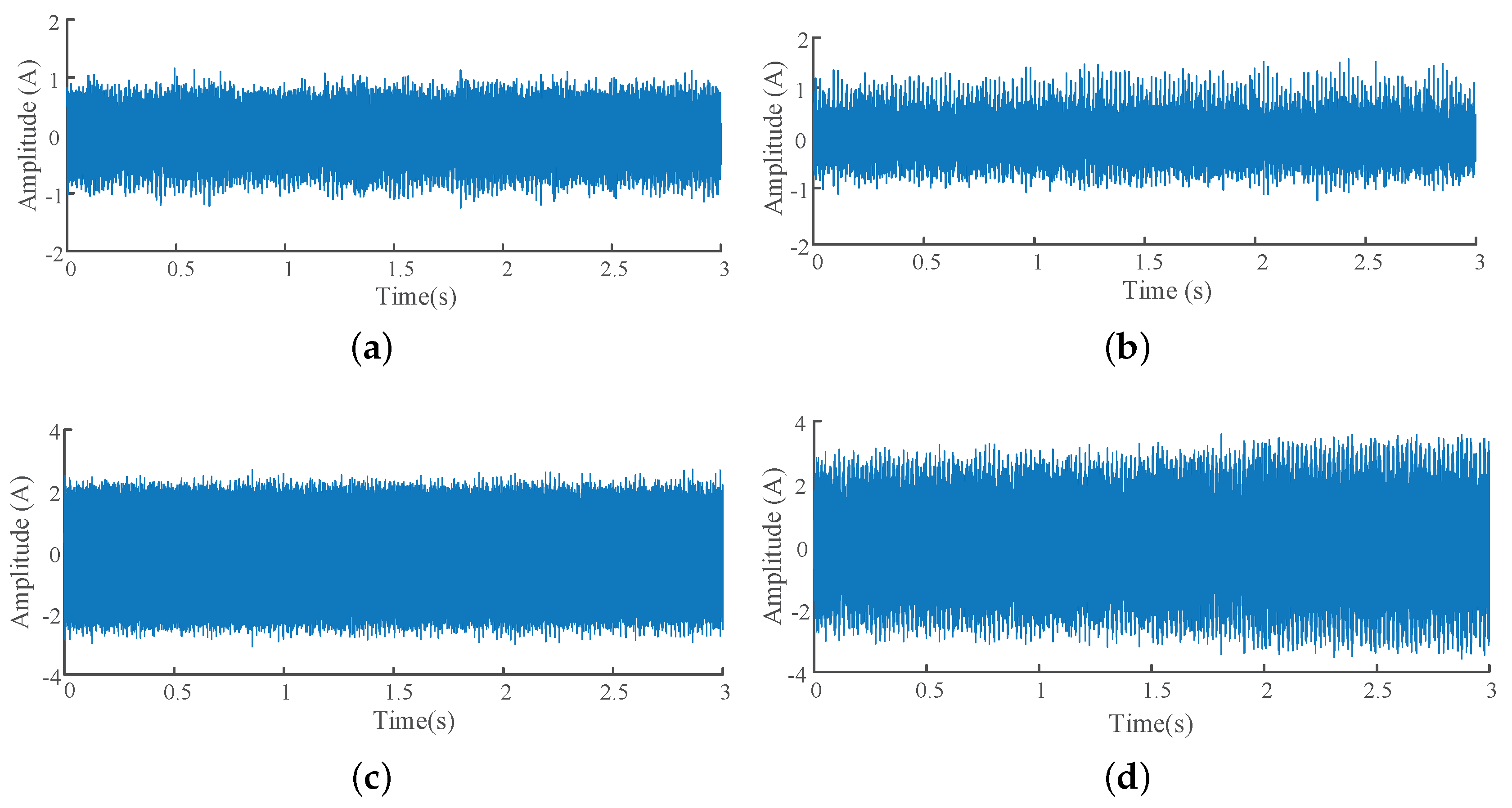
The vibration signals with different degradation degrees are shown in Figure 5, from which it can be seen that there are great differences in the characterization of vibration waveforms under the same working conditions. With the increase of slipper wear, the vibration of piston pump becomes more and more intense, and the amplitude of vibration signal is larger and larger.
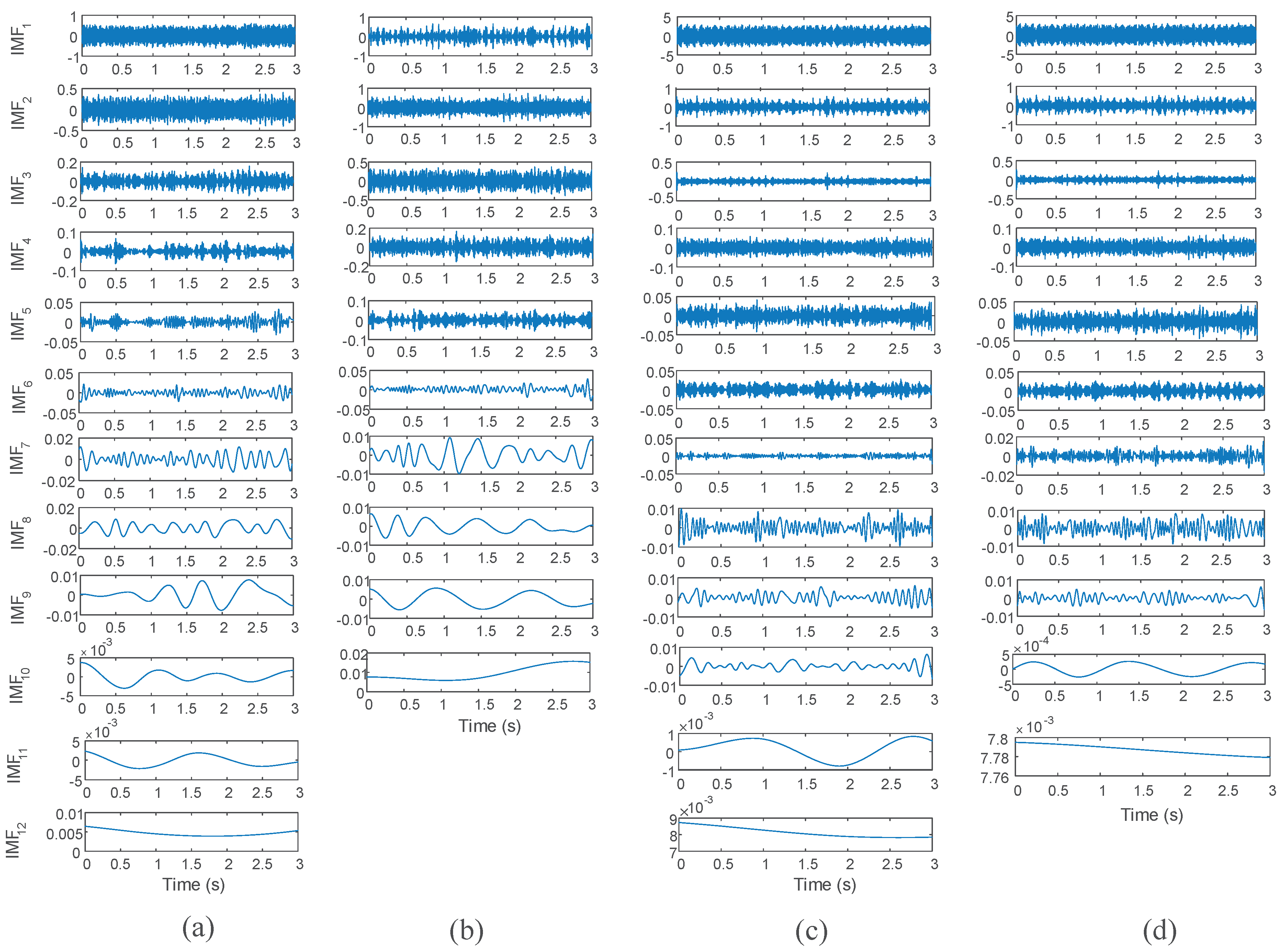
The vibration data of the tested pump under different states are selected and decomposed by ICEEMDAN, and the results are shown in Figure 6. The ICEEMDAN algorithm is used to decompose the vibration signals of four states into respective IMFs and a residual component for model development. The IMFs generated by ICEEMDAN have different sensitivity to the degrees of degradation. If the IMFs are analyzed directly, it is difficult to get the effective features related to the original signal. The appearance of illusive components will cause the extraction of useless features, increase the dimension of the feature set, and bring difficulties to the subsequent analysis [41]. By comparing correlation coefficients, the effective components in IMFs were screened out. The IMF component with the largest correlation coefficient is selected as the research object in this paper.
Then, the appropriate IMF component is selected by using the correlation coefficient method [42]. The calculation process of the correlation coefficient is shown in Formula (11):
R = n = 0 x n y n n = 0 x 2 n n = 0 y 2 n
where x n is the sequence of effective IMF component, y n is the sequence of the original signal.
The correlation coefficient method can be used to express the correlation between the selected IMF component and the original signal, the correlation coefficient values of the IMF components of the four states are showed in Table 1. The larger the correlation coefficient is, the greater the correlation between the IMF components and the original signal, the more effective information it contains. On the contrary, the IMF component is more likely to be illusive.
From the above table, we can see the correlation coefficient of each IMF component under the four conditions. The IMF 1 component under no wear condition, the IMF 1 component under mild wear condition, the IMF 2 component with moderate wear degree, and the IMF 2 component with severe wear degree are selected respectively, and then the selected IMF is analyzed in time domain, frequency domain, and entropy features.

4.2. Multi-Domain Feature Selection

The selected characteristic parameters of time domain and calculation methods are shown in the Table 2. In the time domain characteristics, the root mean square reflects the irregular continuity of vibration and the energy of signal. The peak–peak value can be used to represent the impact vibration caused by the wear of the the inner edge. The spike degree of vibration signal waveform about piston pump is expressed by peak value. The variance indicates the energy and intensity of vibration signal. The degree to which vibration signals deviates from normal distribution is reflected by skewness and kurtosis.The waveform index is a sensitive and stable parameter, which can well represent the slight damage of slippers with different wear degrees. With the aggravation of wear, the impulsion index and tolerance index increase obviously [43,44,45].
In order to obtain degradation information from the frequency domain of vibration signals, we select F 10 : average frequency, F 11 : frequency variance, F 12 : gravity frequency, F 13 : frequency standard deviation, and statistical indexes about frequency domain in reference [46] are F 14 , F 15 , F 16 in the table. The average frequency reflects the vibration energy in the frequency domain. The frequency variance, F 14 and F 15 , indicate the dispersion or concentration of the spectrum. The position change of the main frequency band is obtained according to gravity frequency, frequency standard deviation, and F 16 . The numerical explanation is shown in Table 3.
s ( i ) is the spectrum value of effective IMF, i = 1 , 2 , 3 , , N , N is the total number of spectral lines, and f i is the frequency value of the i-th spectral line.
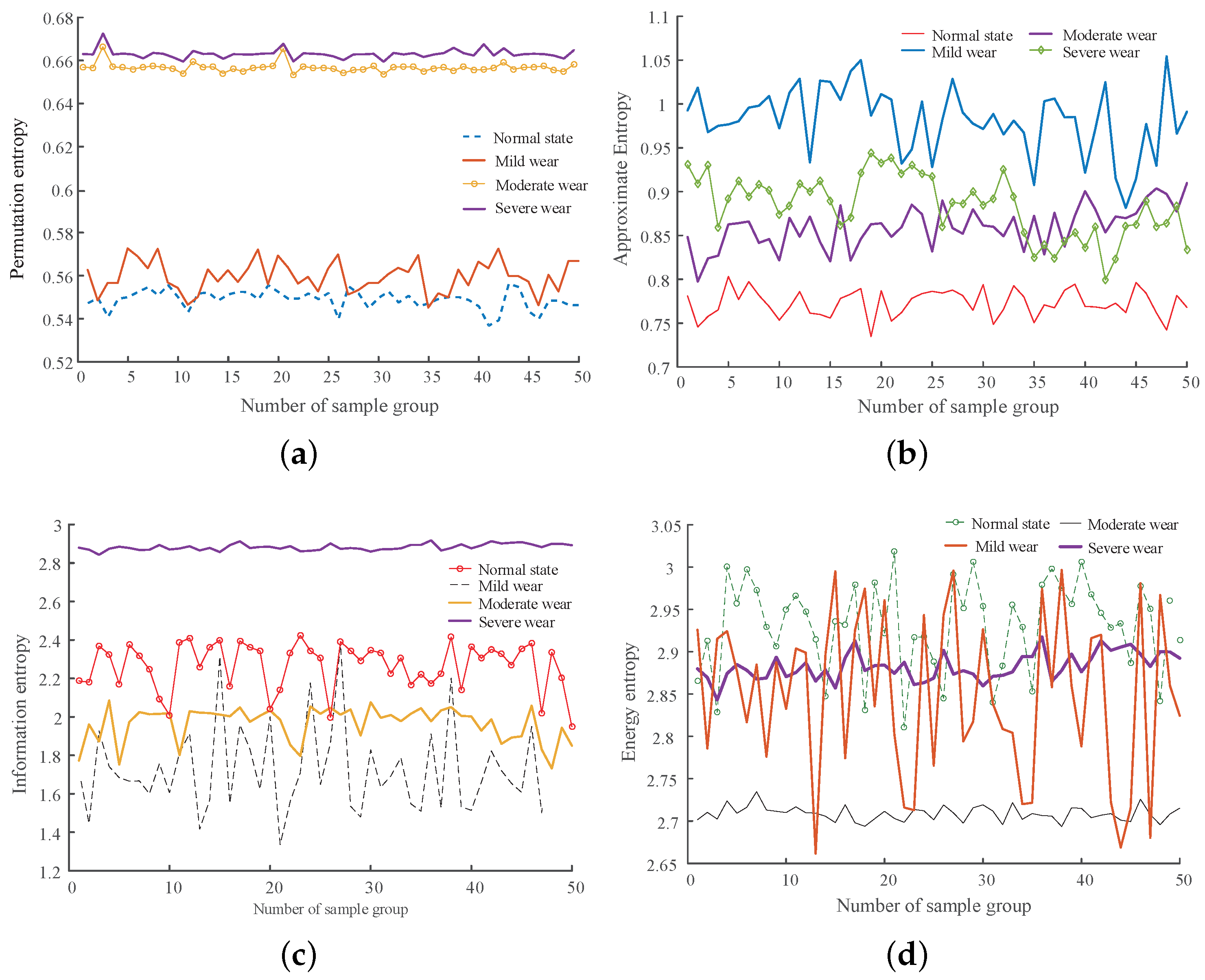
These characteristic values listed in Table 2 and Table 3 represent the degradation trend of the piston pump from different perspectives, which in time domain and frequency domain vary with the different degradation states. In order to further extract the piston pump characteristic information of different degradation state, the permutation entropy [47], approximate entropy [48], information entropy [49], and energy entropy [50] of effective IMFs are calculated, respectively, forming the feature information set based on IMF frequency band. The four entropy features of each degradation state are shown in Figure 7.
It can be seen from Figure 7 that different degradation states have a good hierarchy. With the degree of wear increasing, the vibration signal over time series becomes relatively chaotic and complex, but its entropy values are more stable.

4.3. Feature Filtering by PCA

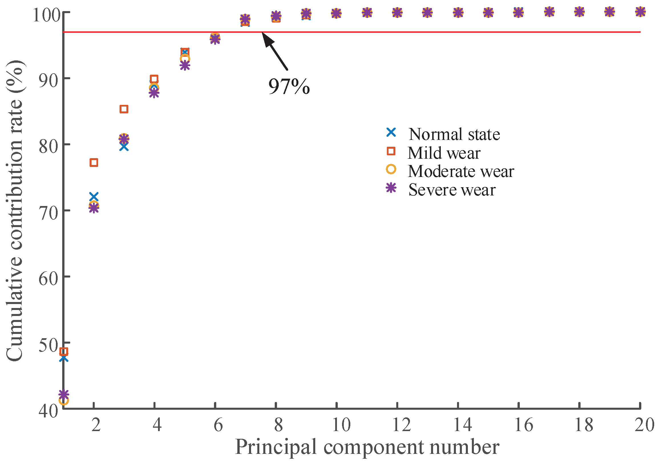
Too high feature dimensions lead to over fitting and some of the features are highly correlated, which will increase the unnecessary calculation burden [51]. Therefore, the PCA algorithm is used in this paper to obtain new low-dimensional features, remove redundant features, and retain the main information of original feature vectors while reducing the complexity of classification and recognition model [52]. The results are shown in Figure 8.
For the convenience of calculation, the coincidence degree of cumulative contribution rate under different degradation states should be high, and we need the same number of principal components in different degradation states [43]. It can be seen from Figure 8 that, when the number of principal components is 6, the cumulative contribution rate of the four degradation states is about 96.4%, and have a high degree of coincidence and contain most of the degradation information of the feature set. When there are too many principal components, the interpretation degree of redundant principal components is smaller than that of a single variable, which will only increase the calculation time and complexity of the model. On the contrary, when there are too few principal components, the whole feature set can not be expressed, and if different degradation states have different numbers of principal components, the calculation will become more complex and reduce the accuracy of model prediction. Therefore, the first six principal components are used to replace the original 20-dimensional degenerate feature vector, which reduces the data dimension and calculation cost. The first six principal components are used as new feature vectors to construct the training set and test set of XGBoost model respectively.

5. Degradation State Recognition with XGBoost

5.1. Parameter Optimization for the XGBoost Model

In order to improve the performance of the model, it is necessary to adjust the XGBoost parameters. The XGBoost algorithm mainly includes three types of parameters: general parameters, Booster parameters, and task parameters. Each type of parameter includes several specific parameter values, among which the booster parameters have a greater impact on the algorithm performance. In this paper, on the basis of fixing other parameters, changing the booster parameters: max depth (the maximum depth of the tree), the min child weight (minimum sum of instance weight needed in a child) and n estimators (number of base classifiers) to find the optimal parameters, which can avoid the over-fitting of the model and improve the model accuracy.
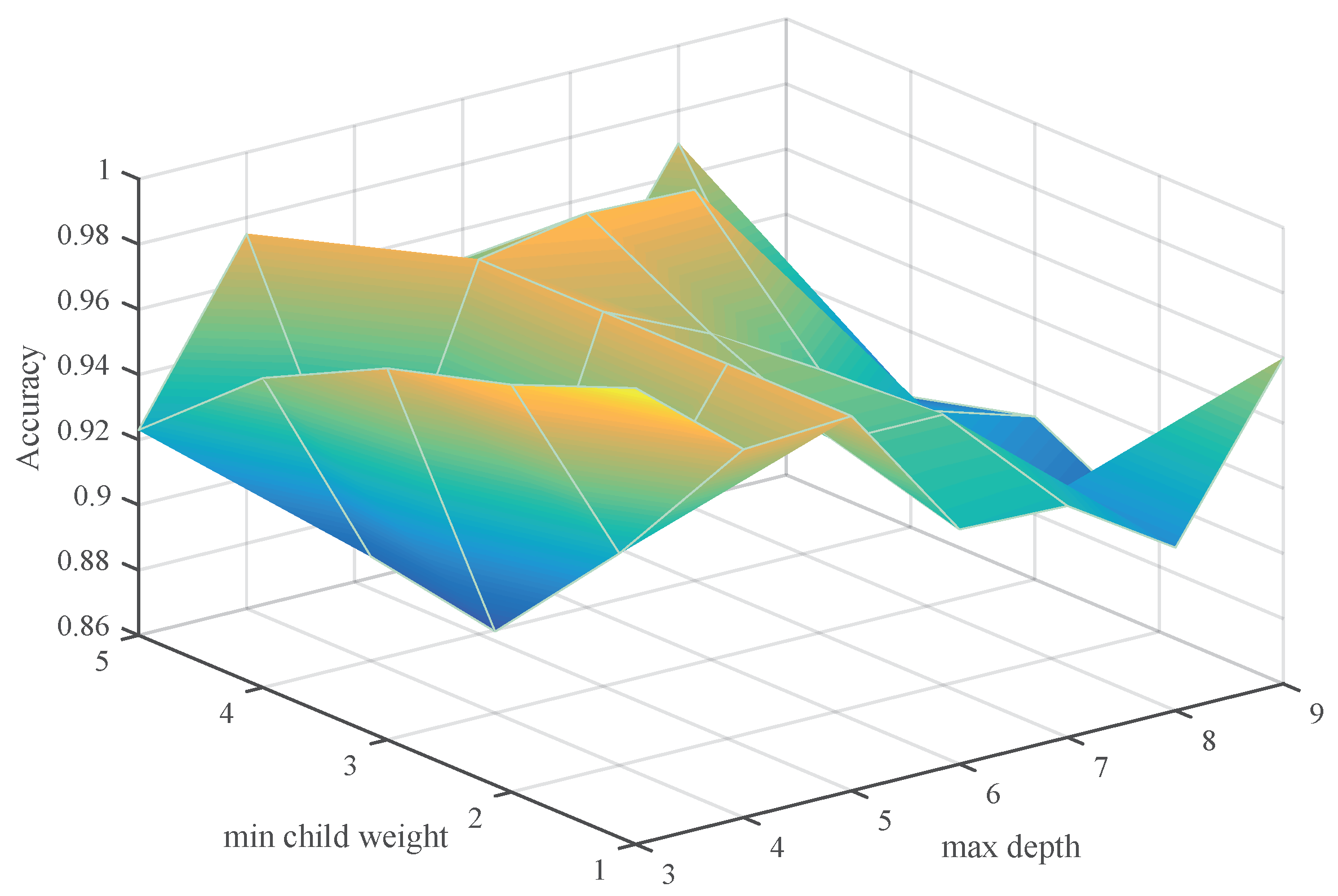
The maximum depth of the trees and the min child weight are two parameters that affect each other. If the parameters are optimized in turn, they will only become disadvantages of local optimization. Moreover, the amount of data in this paper is small; therefore, we can use the grid search to select the maximum depth of the trees and the min child weight at the same time. The results are shown in Figure 9.
When the maximum depth of the tree is 3 and the weight sum of leaf nodes is 1, the average state recognition accuracy is the highest, which is 0.9917. Thus, the max depth = 3 and the min child weight = 1. Fixing the above two parameters, the number of decision trees was selected by logarithmic loss function to evaluate the probability output of XGBoost classifier [53]. The logarithmic loss function is defined as:
σ = 1 N i = 1 N j = 1 M y i j log ( p i j )
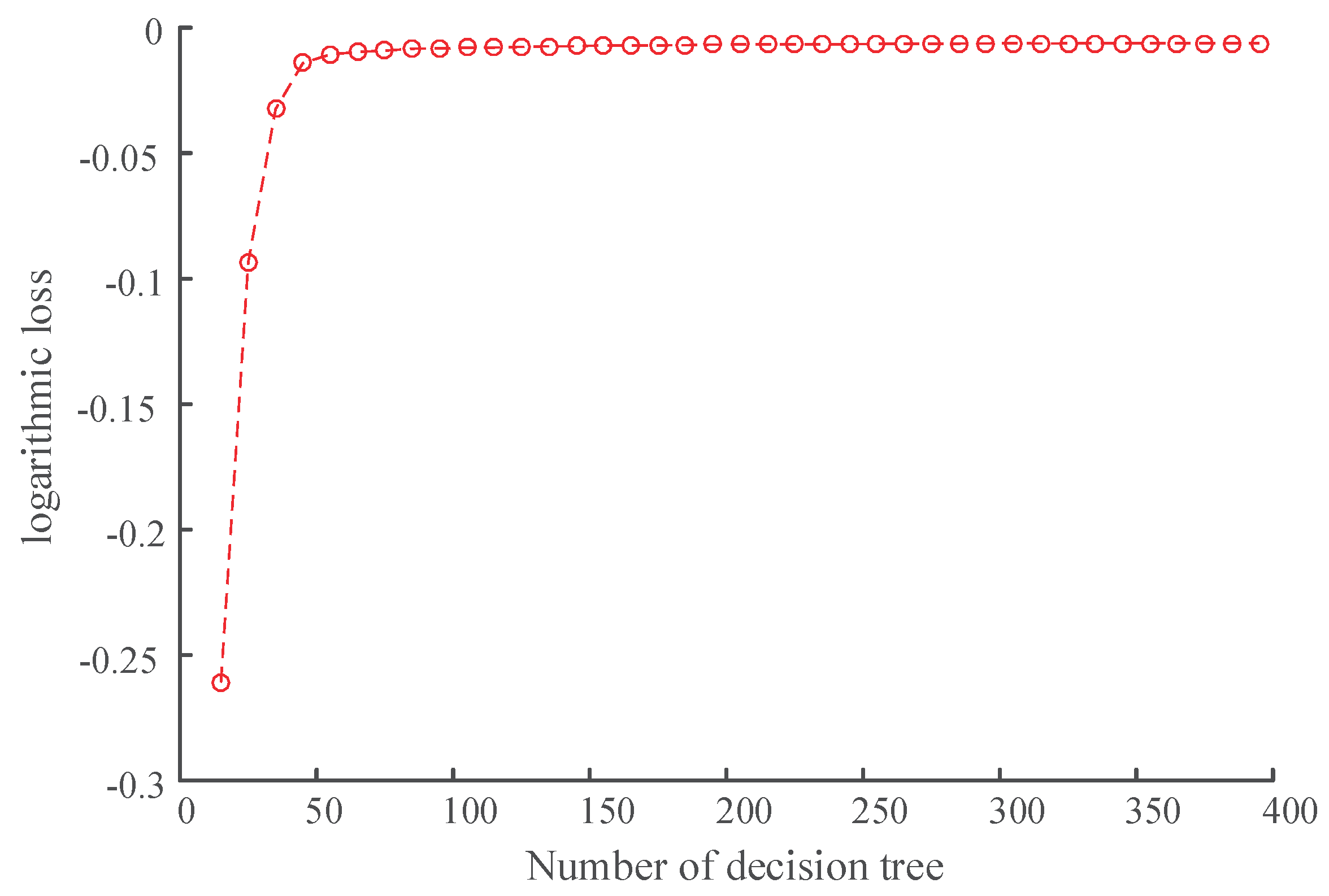
where N is the input sample size, M is the number of categories, y i j represents the real category of the input data points, and p i j is the probability that the i-th data point predicted by the XGBoost classifier belongs to the j-th class. The results are shown in Figure 10.
The closer the value of logarithmic loss is to 0, the higher the accuracy of the classifier is. In this paper, when the number of trees is 167, the logarithmic loss value is −0.0061, which is the largest, so the number of the trees is equal to 167. The parameters for XGBoost are shown in the Table 4, and the remaining parameters are the default values.

5.2. Experimental Results and Analysis

In order to better verify the efficiency and correctness of this method, K-fold cross validation [54] is used to calculate the recognition accuracy of the XGBoost model. The data set is divided into 10 parts, among which six parts were taken as training data, and the remaining four parts were taken as test data in turn for experiments. The average value of recognition accuracy is taken as the final result. Moreover, the method adopted in this paper is also compared with ANN, SVM, and GBDT shown in Table 5. It is found that, when the number of hidden layer neurons of ANN is 12, the effect is better, while the kernel function of SVM is RBF, the penalty coefficient is 4, and gamma is 0.1. By adjusting and optimizing the parameters of GBDT, n estimators = 20, max depth = 3, and min samples split (the minimum number of samples needed when the internal nodes are divided again) = 10.
The above table shows the average accuracy and average calculation time of multiple status recognition verifications. As you can see from the table, the average recognition accuracy of the four algorithms has little difference, possibly because the feature values extracted by the method proposed in this paper have good discrimination—among which SVM and XGBoost have the highest recognition accuracy of 0.997. SVM takes a long calculation time because of the kernel function. Thus, when the performance of the computer is the same, the average decision time of XGBoost is less than that of SVM, which is 0.03 s. Compared with the traditional GBDT model, XGBoost adds the control of model complexity and pruning processing, which makes the trained model difficult to overfitting, and the calculation time is relatively less. The average recognition rate of GBDT is 0.994, but the average decision time is lower than SVM and ANN. ANN needs to iterate repeatedly to get the ideal classification effect, so it has higher average decision time than three other algorithms. In the complex working environment, the vibration data of piston pump are complex and changeable, so it is necessary to extract a variety of characteristics from it to carry out effective diagnosis. Compared with ANN, the diagnostic accuracy of XGBoost can be improved by 0.001 to 0.013, and there is no need for a tedious parameter optimization process. The XGBoost algorithm can not only ensure high diagnosis accuracy but also reduce calculation time. In order to further prove the effectiveness of the present work in this paper, a variety of methods are introduced for comparison. The comparative results are shown in Table 6.
The results are shown in Table: in the case of no data preprocessing, the recognition rate is low due to the influence of noise. Compared with EEMD, after ICEEMDAN preprocessing, the recognition rate will be relatively high. Therefore, the proposed method effectively identifies degraded states. It can maintain mechanical equipment through timely judgment, which has high practical value in the fault diagnosis of piston pump.

6. Conclusions

In this paper, ICEEMDAN is used to denoise the vibration signal of the piston pump, PCA is used to reduce the feature dimension, and the state recognition based on XGBoost is carried out to identify the wear state and category of the piston pump slipper. The experimental results show that:
a.
The ICEEMDAN can decompose the vibration signal of piston pump adaptively, improve the decomposition efficiency, and suppress phenomena of mode mixing. It is feasible to select an effective IMF component by using correlation coefficient.
b.
Through time domain, frequency domain, and entropy, the deterioration process of piston pump can be tracked and identified comprehensively. The PCA is used to reduce data dimension and calculation cost, which improves the accuracy and efficiency of state identification.
c.
The average recognition accuracy of slipper wear state of piston pump based on ICEEMDAN and XGBoost is 99.7%. Compared with ANN, GBDT, and SVM algorithm, XGBoost identifies four different wear states better and saves the computing time, which highlights the advantages of XGBoost after parameter optimization in pattern recognition.

Author Contributions

All the authors contributed to the original idea and design of the study, to the analysis, to the drafting of the manuscript, and reading and approving the final version. Conceptualization, R.G. and Z.Z.; methodology, R.G.; validation, R.G., T.W., and Z.Z.; formal analysis, G.L. and D.G.; resources, R.G. and J.Z.; data curation, Z.Z.; writing—original draft preparation, Z.Z.; writing—review and editing, R.G. and Z.Z.; visualization, Z.Z.; Software, Z.Z. and T.W.; supervision, T.W.; project administration, R.G. and J.Z.; funding acquisition, R.G., J.Z., and D.G. All authors have read and agreed to the published version of the manuscript.

Funding

This research was funded by the National Key Research and Development Program of China (Grant No. 2019YFB2005204), the National Natural Science Foundation of China (Grant No.52075469, 51675461, 11673040), the Key Research and Development Program of Hebei Province (Grant No. 19273708D), and the Open Foundation of the State Key Laboratory of Fluid Power and Mechatronic Systems (Grant No. GZKF-201922).

Acknowledgments

The authors would like to acknowledge the support provided by Yanshan University.

Conflicts of Interest

The authors declare no conflict of interest.

References

  1. Lan, Y.; Hu, J.; Huang, J.; Niu, L.; Zeng, X.; Xiong, X.; Wu, B. Fault Diagnosis on Slipper Abrasion of Axial Piston Pump based on Extreme Learning Machin. Measurement 2010, 124, 378–385. [Google Scholar] [CrossRef]
  2. Guo, S.; Chen, J.; Lu, Y.; Yan, W.A.N.G.; Hongkang, D.O.N.G. Hydraulic piston pump in civil aircraft: Current status, future directions and critical technologies. Chin. J. Aeronaut. 2020, 33, 16–30. [Google Scholar] [CrossRef]
  3. Son, Y.K.; Savage, G.J. A New Sample-Based Approach to Predict System Performance Reliability. IEEE Trans. Reliab. 2008, 52, 322–330. [Google Scholar]
  4. Zamanian, A.H.; Ohadi, A. Wear prediction for metals. Tribol. Int. 1997, 30, 377–383. [Google Scholar]
  5. Lin, J.S.; Chen, Q. Fault diagnosis of rolling bearings based on multifractal detrended fluctuation analysis and Mahalanobis distance criterion. Mech. Syst. Signal Process. 2013, 38, 515–533. [Google Scholar] [CrossRef]
  6. Xu, B.; Zhang, J.; Yang, H. Investigation on structural optimization of anti-overturning slipper of axial piston pump. Sci. China Technol. Sci. 2012, 55, 3010–3018. [Google Scholar] [CrossRef]
  7. Liu, H.; Yuan, S.H.; Jing, C.B.; Zhao, Y.M. Effects of Wear Profile and Elastic Deformation on the Slipper’s Dynamic Characteristics. J. Mech. Eng. 2012, 28, 608–621. [Google Scholar] [CrossRef]
  8. Tian, Z.K.; Li, H.R.; Sun, J.; Li, B.C. Degradation state identification method of hydraulic pump based on improved MF-DFA and SSM-FM. Chin. J. Sci. Instrum. 2016, 37, 1851–1860. [Google Scholar]
  9. Xiao, W.B.; Chen, J.; Zhou, Y.; Wang, Z.Y.; Zhao, F.G. Wavelet packet transform and hidden Markov model based bearing performance degradation assessment. J. Mech. Eng. 2011, 30, 32–35. [Google Scholar]
  10. Singh, D.S.; Zhao, Q. Pseudo-fault signal assisted EMD for fault detection and isolation in rotating machines. Mech. Syst. Signal Process. 2016, 81, 202–218. [Google Scholar] [CrossRef]
  11. Lei, Y.G. Machinery Fault Diagnosis Based on Improved Hilbert-Huang Transform. J. Mech. Eng. 2011, 47, 71–77. [Google Scholar] [CrossRef]
  12. Lei, Y.G.; He, Z.J.; Zi, Y.Y. Application of the EEMD method to rotor fault diagnosis of rotating machinery. Mech. Syst. Signal Process. 2009, 23, 1327–1338. [Google Scholar] [CrossRef]
  13. Lee, D.-H.; Ahn, J.-H.; Koh, B.-H. Fault Detection of Bearing Systems through EEMD and Optimization Algorithm. Sensors 2017, 17, 2477. [Google Scholar] [CrossRef] [Green Version]
  14. Wu, Z.H.; Huang, N.E. Ensemble empirical mode decomposition: A noise-assisted data analysis method. Adv. Adapt. Data Anal. 2009, 1, 1–41. [Google Scholar] [CrossRef]
  15. Torres, M.E.; Colominas, M.A.; Schlotthauer, G.; Flandrin, P. A complete ensemble empirical mode decomposition with adaptive noise. In Proceedings of the 2011 IEEE International Conference on Acoustics, Speech and Signal Processing (ICASSP), Prague, Czech Republic, 22–27 May 2011; pp. 4144–4147. [Google Scholar]
  16. Tian, Z.K.; Li, H.R.; Gu, H.Q.; Xu, B.H. Degradation status identification of a hydraulic pump based on local characteristic-scale decomposition and JRD. J. Vib. Shock 2016, 35, 54–59. [Google Scholar]
  17. Wang, B.; Li, H.R.; Chen, Q.H.; Xu, B.H. Rolling Bearing Performance Degradative State Recognition Based on Mathematical Morphological Fractal Dimension and Fuzzy Center Means. Acta Armamentarii 2015, 36, 1982–1990. [Google Scholar]
  18. Zhang, S.; Li, W. Bearing Condition Recognition and Degradation Assessment under Varying Running Conditions Using NPE and SOM. Math. Probl. Eng. 2014, 9, 781583. [Google Scholar] [CrossRef]
  19. Si, L.; Wang, Z.; Liu, X.; Tan, C. A sensing identification method for shearer cutting state based on modified multi-scale fuzzy entropy and support vector machine. Eng. Appl. Artif. Intell. 2019, 78, 86–101. [Google Scholar] [CrossRef]
  20. Ji, Y.; Sun, S. Multitask multiclass support vector machines: Model and experiments. Pattern Recognit. 2013, 46, 914–924. [Google Scholar] [CrossRef]
  21. Azadeh, A.; Saberi, M.; Kazem, A.; Ebrahimipour, V.; Nourmohammadzadeh, A.; Saberi, Z. A flexible algorithm for fault diagnosis in a centrifugal pump with corrupted data and noise based on ANN and support vector machine with hyper-parameters optimization. Appl. Soft Comput. 2013, 13, 1478–1485. [Google Scholar] [CrossRef]
  22. Siddiqui, S.A.; Verma, K.; Niazi, K.R.; Fozdar, M. Real-Time Monitoring of Post-Fault Scenario for Determining Generator Coherency and Transient Stability through ANN. IEEE Trans. Ind. Appl. 2017, 54, 685–692. [Google Scholar] [CrossRef]
  23. Wang, Y.S.; Liu, N.N.; Guo, H.; Wang, X.L. An engine-fault-diagnosis system based on sound intensity analysis and wavelet packet pre-processing neural network. Eng. Appl. Artif. Intell. 2020, 94, 103765. [Google Scholar] [CrossRef]
  24. Yan, X.; Jia, M. A novel optimized SVM classification algorithm with multi-domain feature and its application to fault diagnosis of rolling bearing. Neurocomputing 2018, 313, 47–64. [Google Scholar] [CrossRef]
  25. Wang, S.; Xiang, J.; Zhong, Y.; Tang, H. A data indicator-based deep belief networks to detect multiple faults in axial piston pumps. Mech. Syst. Signal Process. 2018, 112, 154–170. [Google Scholar] [CrossRef]
  26. Chen, C.-H.; Zhao, W.D.; Pang, T.; Lin, Y.-Z. Virtual metrology of semiconductor PVD process based on combination of tree-based ensemble model. ISA Trans. 2020, 103, 192–202. [Google Scholar] [CrossRef]
  27. Ampomah, E.K.; Qin, Z.; Nyame, G. Evaluation of Tree-Based Ensemble Machine Learning Models in Predicting Stock Price Direction of Movement. Information 2020, 11, 332. [Google Scholar] [CrossRef]
  28. Adler, W.; Potapov, S.; Lausen, B. Classification of repeated measurements data using tree-based ensemble methods. Comput. Stat. 2011, 26, 355–369. [Google Scholar] [CrossRef]
  29. Kotsiantis, S. Combining bagging, boosting, rotation forest and random subspace methods. Artif. Intell. Rev. 2011, 35, 223–240. [Google Scholar] [CrossRef]
  30. Chen, T.; Guestrin, C. Xgboost: A scalable tree boosting system. In Proceedings of the 22nd ACM SIGKDD International Conference on Knowledge Discovery and Data Mining, San Francisco, CA, USA, 13–17 August 2016; pp. 785–794. [Google Scholar]
  31. Friedman, J.H. Greedy Function Approximation: A Gradient Boosting Machine. Ann. Stat. 2001, 29, 1189–1232. [Google Scholar] [CrossRef]
  32. Wu, Z.; Wang, X.; Jiang, B. Fault Diagnosis for Wind Turbines Based on ReliefF and eXtreme Gradient Boosting. Appl. Sci 2020, 10, 3258. [Google Scholar] [CrossRef]
  33. Debaditya, C.; Hazem, E. Advanced machine learning techniques for building performance simulation: A comparative analysis. J. Build. Perform. Simul. 2019, 12, 193–207. [Google Scholar]
  34. Colominas, M.A.; Schlotthauer, G.; Torres, M.E. Improved complete ensemble EMD: A suitable tool for biomedical signal processing. Biomed. Signal Process. Control. 2014, 14, 19–29. [Google Scholar] [CrossRef]
  35. Ji, N.; Ma, L.; Dong, H.; Zhang, X. Selection of Empirical Mode Decomposition Techniques for Extracting Breathing Rate From PPG. IEEE Signal Process. Lett. 2019, 26, 592–596. [Google Scholar]
  36. Ali, M.; Prasad, R. Significant wave height forecasting via an extreme learning machine model integrated with improved complete ensemble empirical mode decomposition. Renew. Sustain. Energy Rev. 2019, 104, 281–295. [Google Scholar] [CrossRef]
  37. Huang, N.E.; Shen, Z.; Long, S.R.; Wu, M.C.; Shih, H.H.; Zheng, Q.; Yen, N.C.; Tung, C.C.; Liu, H.H. The empirical mode decomposition and the Hilbert spectrum for nonlinear and non-stationary time series analysis. Proc. Math. Phys. Eng. Sci. 1998, 454, 903–995. [Google Scholar] [CrossRef]
  38. Li, Y.; Xu, F. Signal processing and identification on the surface of Pinus massoniana Lamb. glulam using acoustic emission and improvement complete ensemble empirical mode decomposition with adaptive noise. Measurement 2019, 148, 106978. [Google Scholar] [CrossRef]
  39. Wang, L.; Zhou, D.; Zhang, H.; Zhang, W.; Chen, J. Application of Relative Entropy and Gradient Boosting Decision Tree to Fault Prognosis in Electronic Circuits. Symmetry 2018, 10, 495. [Google Scholar] [CrossRef] [Green Version]
  40. Chen, Y.; Wang, X.; Jung, Y.H.; Abedi, V.; Zand, R.; Bikak, M.; Adibuzzaman, M. Classification of short single lead electrocardiograms (ECGs) for atrial fibrillation detection using piecewise linear spline and XGBoost. Physiol. Meas. 2018, 39, 104006. [Google Scholar] [CrossRef]
  41. Zheng, H.M.; Dang, C.L.; Gu, S.M.; Peng, D.; Chen, K. A quantified self-adaptive filtering method: Effective IMFs selection based on CEEMD. Meas. Sci. Technol. 2018, 29, 085701. [Google Scholar] [CrossRef]
  42. Jiang, L.; Li, B.; Li, X.J. An Improved HHT Method and its Application in Fault Diagnosis of Roller Bearing. Appl. Mech. Mater. 2013, 273, 264–268. [Google Scholar] [CrossRef]
  43. Lu, C.; Wang, S.; Maids, V. Fault severity recognition of aviation piston pump based on feature extraction of EEMD paving and optimized support vector regression model. Aerosp. Sci. Technol. 2017, 67, 105–117. [Google Scholar] [CrossRef]
  44. Eriştia, H.; Uçarb, A.; Demir, Y. Wavelet-based feature extraction and selection for classification of power system disturbances using support vector machines. Electr. Power Syst. Res. 2010, 80, 743–752. [Google Scholar] [CrossRef]
  45. Hasan, M.J.; Kim, J.; Kim, C.H.; Kim, J.-M. Health State Classification of a Spherical Tank Using a Hybrid Bag of Features and K-Nearest Neighbor. Appl. Sci. 2020, 10, 2525. [Google Scholar] [CrossRef] [Green Version]
  46. Lei, Y.G.; He, Z.J.; Zi, Y.Y.; Hu, Q. Fault diagnosis of rotating machinery based on multiple ANFIS combination with Gas. Mech. Syst. Signal Process. 2007, 21, 2280–2294. [Google Scholar] [CrossRef]
  47. Bandt, C.; Pompe, B. Permutation Entropy: A Natural Complexity Measure for Time Series. Phys. Rev. Lett. 2002, 88, 174102. [Google Scholar] [CrossRef]
  48. Jiang, Z.; Deng, A. Identification of Rotating Machinery Rub and Impact Fault Using Hurst Exponent and Approximate Entropy as Characteristic Parameters of Acoustic Emission. Proc. CSEE 2010, 30, 96–102. [Google Scholar]
  49. Li, J.L.; Huang, S.H. Fault Diagnosis of a Rotary Machine Based on Information Entropy and Rough Set. Int. J. Plant Eng. Manag. 2007, 12, 199–206. [Google Scholar]
  50. Zhu, L.D.; Liu, C.F.; Ju, C.Y.; Guo, M. Vibration recognition for peripheral milling thin-walled workpieces using sample entropy and energy entropy. Int. J. Adv. Manuf. Technol. 2020, 108, 3251–3266. [Google Scholar] [CrossRef]
  51. Bect, P.; Simeu-Abazi, Z.; Maisonneuve, P.L. Diagnostic and decision support systems by identification of abnormal events: Application to helicopters. Aerosp. Sci. Technol. 2015, 46, 339–350. [Google Scholar] [CrossRef]
  52. Wan, X.; Wang, D.; Tse, P.W.; Xu, G.; Zhang, Q. A critical study of different dimensionality reduction methods for gear crack degradation assessment under different operating conditions. Measurement 2016, 78, 138–150. [Google Scholar] [CrossRef]
  53. Hitchcock, J.M. Fractal Dimension and Logarithmic Loss Unpredictability. Theor. Comput. 2003, 304, 431–441. [Google Scholar] [CrossRef] [Green Version]
  54. Rodriguez, J.D.; Perez, A.; Lozano, J.A. Sensitivity Analysis of k-Fold Cross Validation in Prediction Error Estimation. IEEE Trans. Pattern Anal. Mach. Intell. 2010, 32, 569–575. [Google Scholar] [CrossRef] [PubMed]
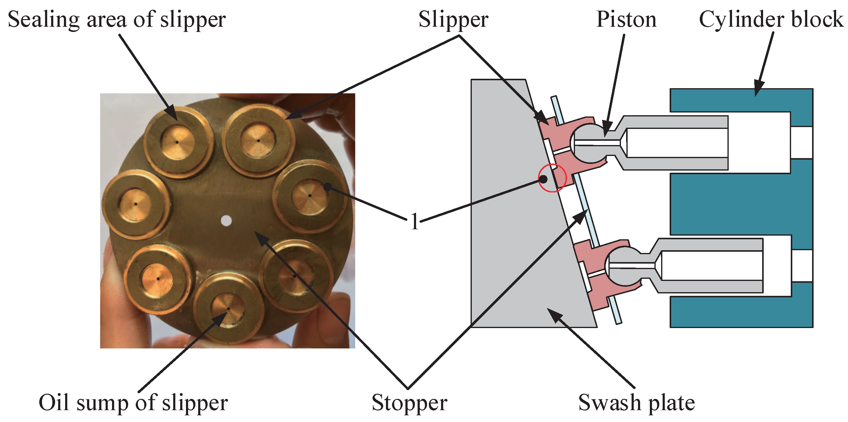
Figure 1. Structure of slipper pair. 1 is the inner edge of the slipper.
Applsci 10 06593 g001
Figure 2. An overview of the proposed methods and analysis steps.
Applsci 10 06593 g002
Figure 3. Flow chart of XGBoost.
Applsci 10 06593 g003
Figure 4. Test bench physical map.
Applsci 10 06593 g004
Figure 5. Vibration signals with four wear degrees. (a) vibration signal of slipper under normal condition; (b) vibration signal of slipper with slight wear; (c) vibration signal of slipper under moderate wear; (d) vibration signal of slipper under severe wear.
Applsci 10 06593 g005
Figure 6. Decomposition results of ICEEMDAN. (a) the vibration signal under normal state are decomposed by ICEEMDAN; (b) the vibration signal under slight wear are decomposed by ICEEMDAN; (c) the vibration signal under moderate wear are decomposed by ICEEMDAN; (d) the vibration signal under severe wear are decomposed by ICEEMDAN.
Applsci 10 06593 g006
Figure 7. Entropy characteristics of four wear states. (a) permutation entropy in different wear states; (b) approximate entropy under different wear states; (c) information entropy under different wear states; (d) energy entropy under different wear conditions.
Applsci 10 06593 g007
Figure 8. Cumulative contribution rate of different principal components under four wear states.
Applsci 10 06593 g008
Figure 9. The relationship between recognition accuracy and max depth, min child weight.
Applsci 10 06593 g009
Figure 10. Determination of the number of trees.
Applsci 10 06593 g010
Table 1. The correlation coefficient values of the IMF components of the four states.
Status of the SlippersNo WearMild WearModerate WearSevere Wear
IMF 1 0.9440.8910.5930.505
IMF 2 0.7620.7870.9040.994
IMF 3 0.4230.1860.4150.523
IMF 4 0.1960.1190.1130.109
IMF 5 0.1350.5000.0340.011
IMF 6 0.3290.0930.0080.003
IMF 7 0.1560.0280.0060.002
IMF 8 0.0680.0080.0040.000
IMF 9 0.0070.0040.0070.000
IMF 10 0.0040.0080.0080.008
IMF 11 0.0030.0080.000
IMF 12 0.0000.004
Table 2. Numerical explanation of time domain.
Time Domain CharacteristicExpression
Root mean square F 1 = 1 N i = 1 N x 2 ( i )
Peak index F 2 = max x F 1
Peak-peak index F 3 = max x min x
Skewness index F 4 = i = 1 N ( x ( i ) x ¯ ) 3 N × F 1 3
Variance F 5 = 1 N i = 1 N x i x ¯ 2
Tolerance index F 6 = F 1 1 N i = 1 N x i
Waveform index F 7 = max ( x ) x ¯
Kurtosis index F 8 = i = 1 N x ( i ) x ¯ 4 N × F 1 4
Impulsion index F 9 = max ( x ) 1 N i = 1 N x i
where x is the selected effective IMF, x ¯ = 1 N i = 1 N x ( i ) .
Table 3. Numerical explanation of frequency domain.
Frequency Domain CharacteristicExpressionFrequency Domain CharacteristicExpression
F 10 1 N i = 1 N s i F 11 i = 1 N ( s ( i ) F 10 ) 2
F 12 i = 1 N f i s ( i ) i = 1 N s ( i ) F 13 i = 1 N ( f i F 12 ) 2 s ( i ) N
F 14 i = 1 N ( s ( i ) F 10 ) 3 N ( F 11 ) 3 F 15 i = 1 N ( s ( i ) F 10 ) 4 N × F 11 2
F 16 i = 1 N f i 2 s ( i ) i = 1 N s ( i )
Table 4. Parameters for XGBoost.
ParameterNumerical Value
Max depth3
Min child weight1
N estimators167
Objectivemulti: softmax
Table 5. Comparison of degradation state recognition results.
Classification MethodAverage Recognition AccuracyAverage Decision Time (s)
ANN0.9910.094
SVM0.9970.012
GBDT0.9940.006
XGBoost0.9970.003
Table 6. Performance comparison for different methods.
NumberFeature Extraction MethodFeature Reduction MethodClassification TechniqueRecognition Rate (%)
1EEMD, Multi-domain features (time domain, frequency domain, entropy)PCAGBDT98.2
2EEMD, Multi-domain featuresPCASVM98.6
3EEMD, Multi-domain featuresXGBoost92.4
4EEMD, Multi-domain featuresPCAXGBoost97.1–100
5Multi-domain featuresPCAXGBoost69.5
6ICEEMDAN, Multi-domain featuresXGBoost94.5–99.2
Present workICEEMDAN, Multi-domain featuresPCAXGBoost98.3–100