Factors That Affect Liquefaction-Induced Lateral Spreading in Large Subduction Earthquakes


Abstract
1. Introduction
2. Background of Lateral Spreading in Subduction Earthquakes
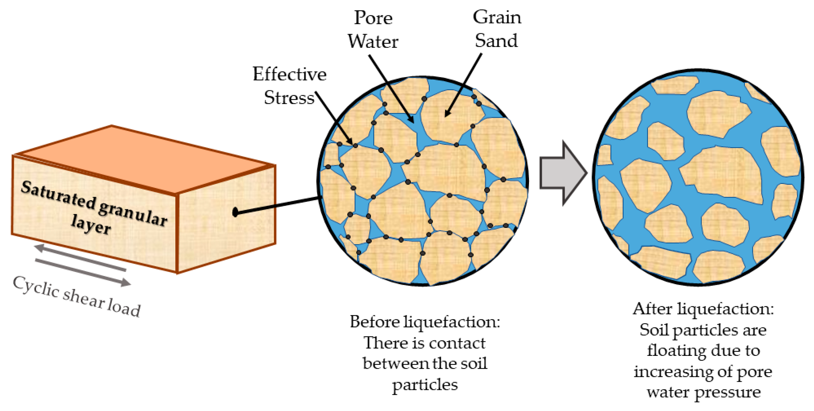
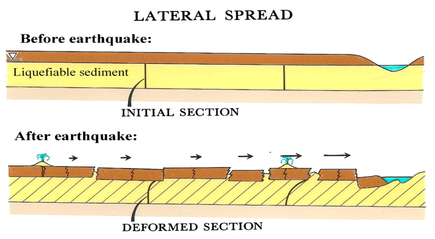
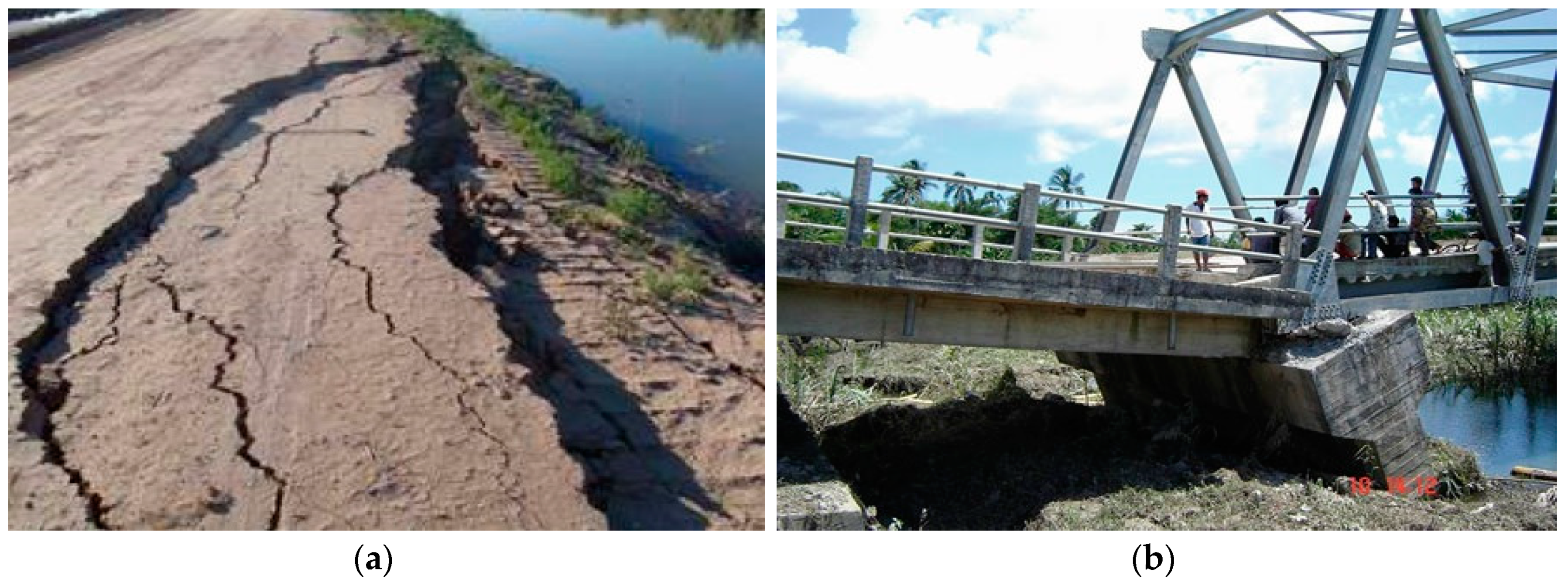
2.1. Liquefaction and Lateral Spreading
2.2. Lateral Spreading Prediction Models
2.3. Current Models and Large-Magnitude Subduction Earthquakes
3. Validation of the Numerical Methodology
3.1. Validation with Centrifuge Tests
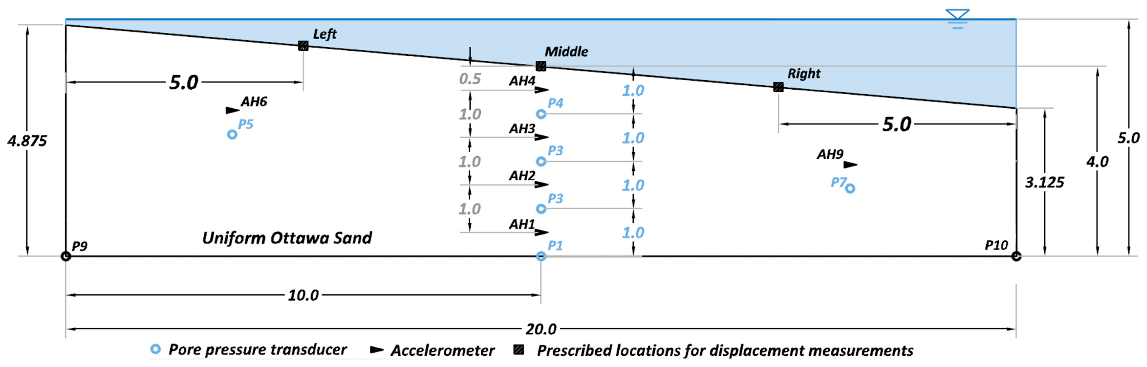
3.1.1. General Description of the Centrifuge Tests
3.1.2. Model Input Parameters
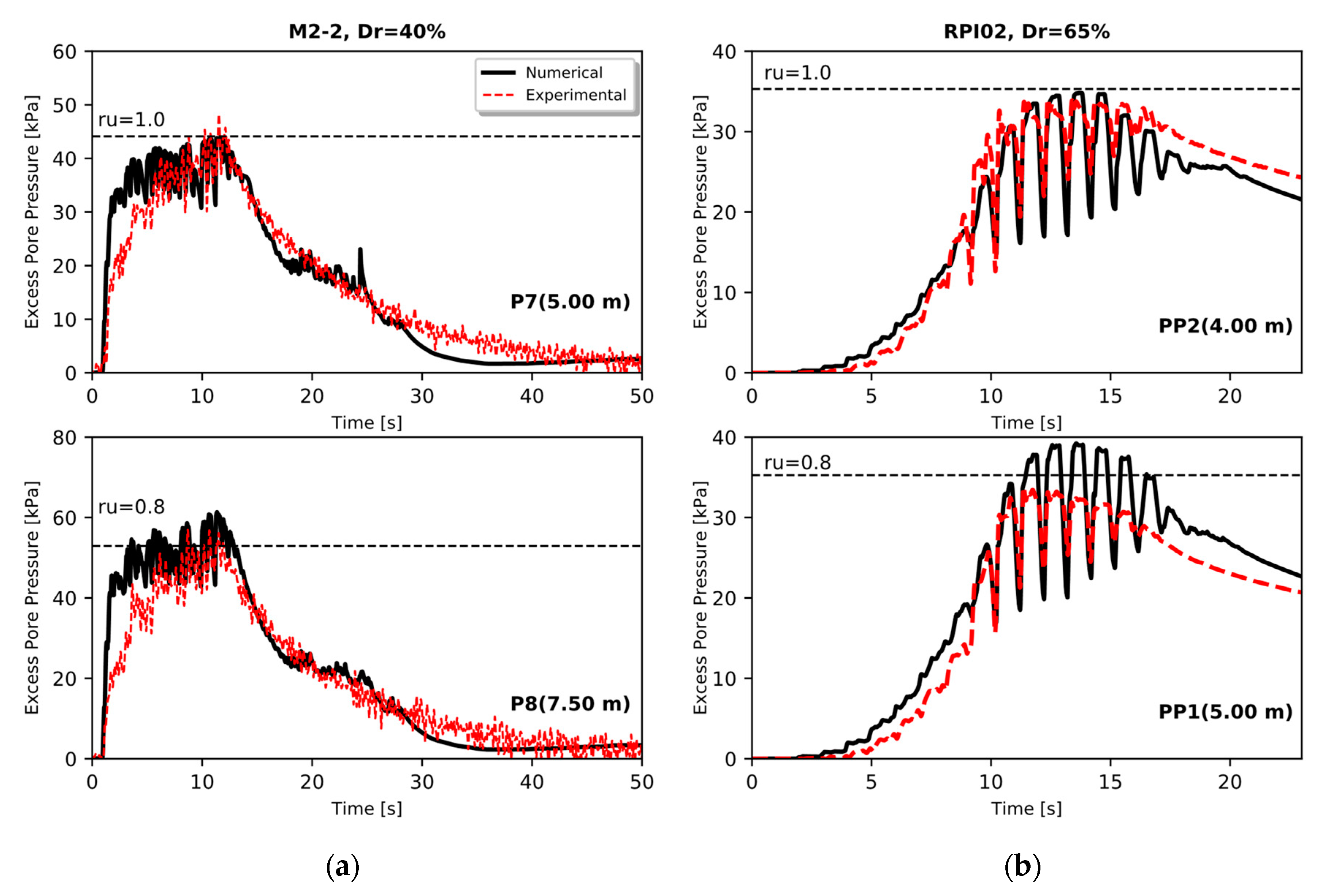
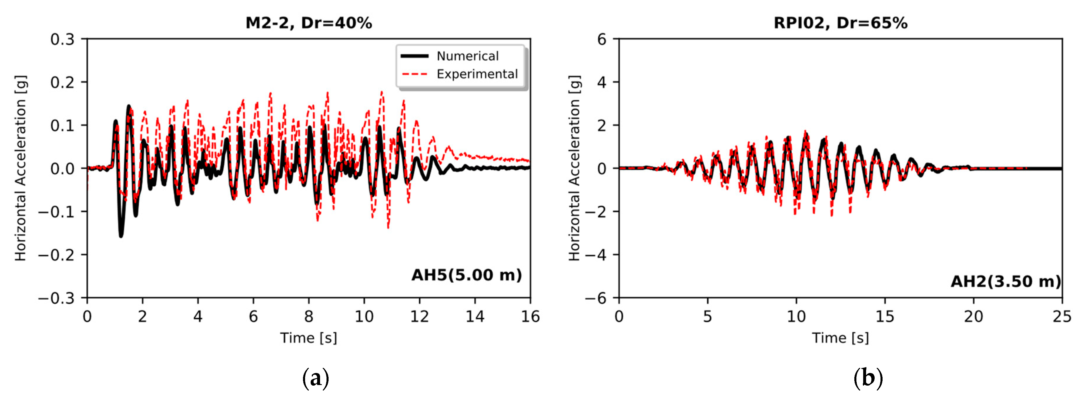
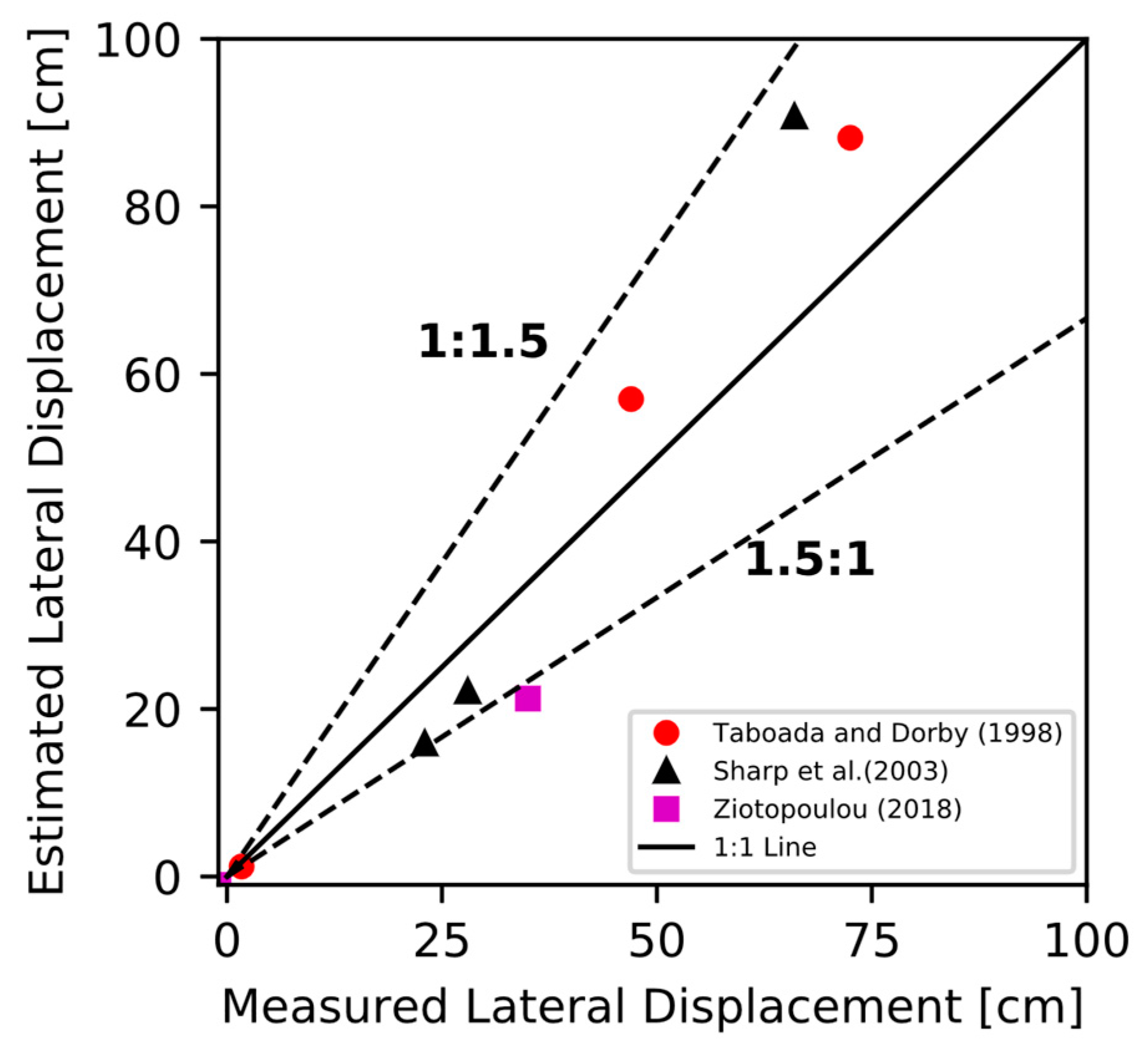
3.1.3. Comparison of Results
3.2. Validation with Historical Cases
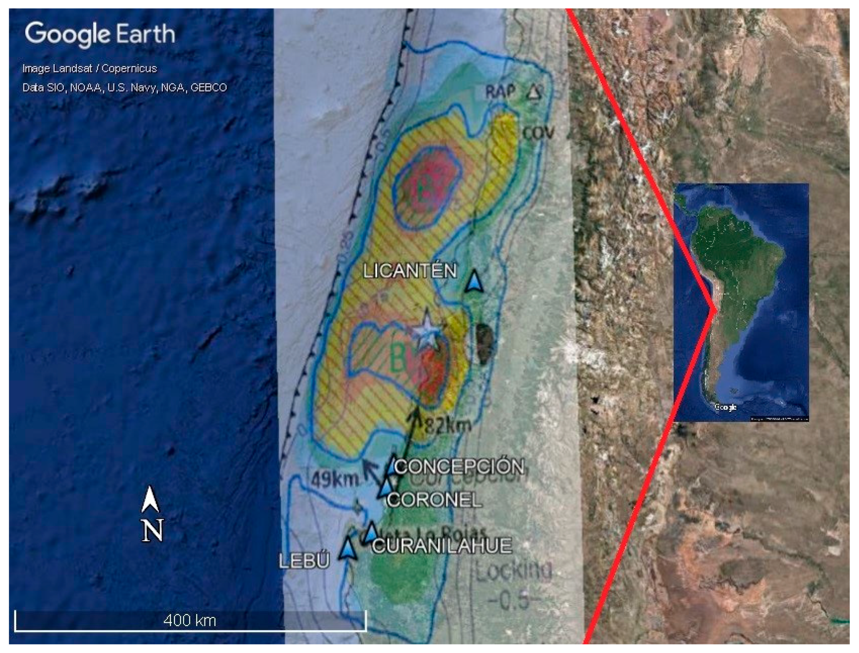
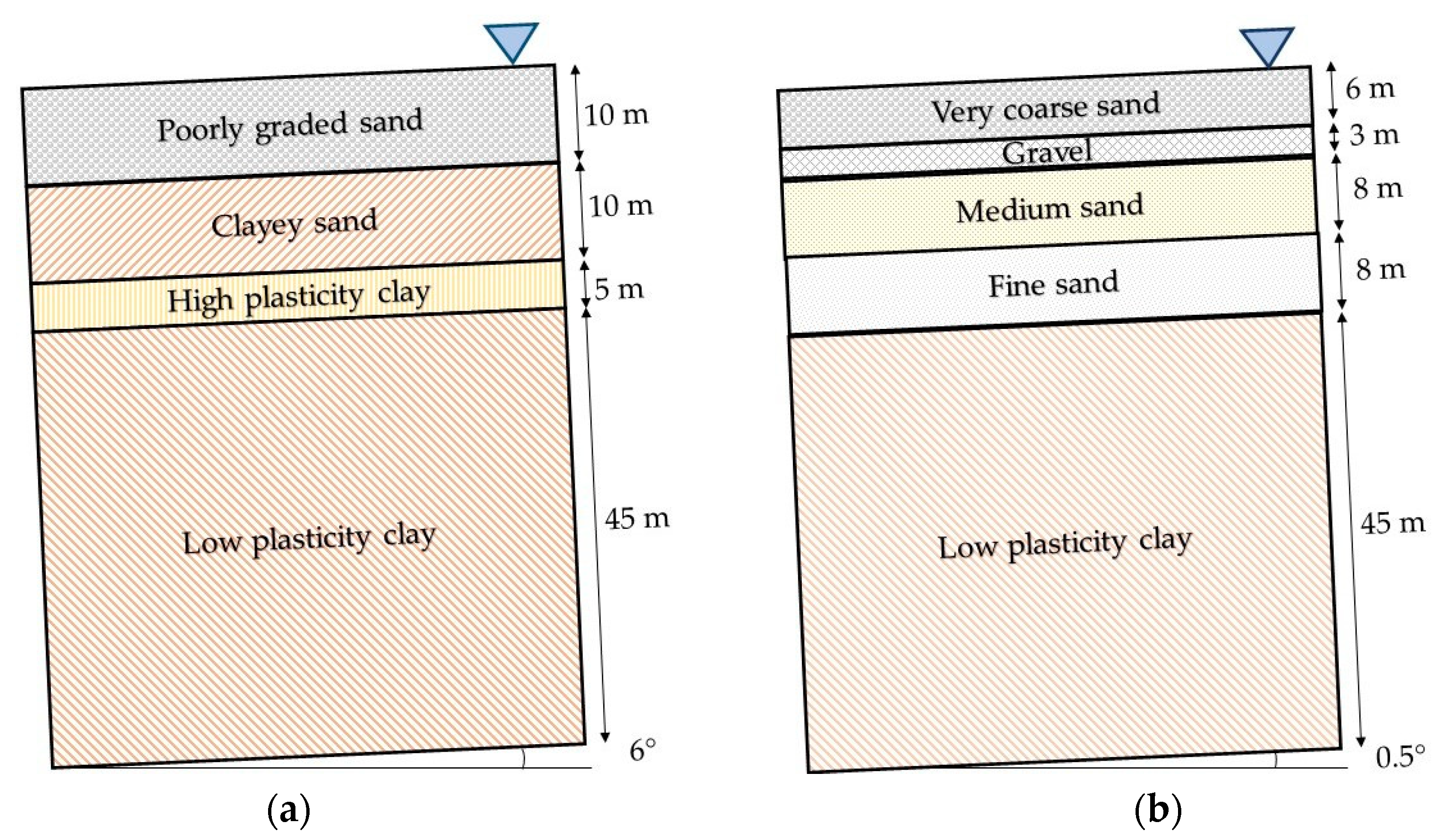
3.2.1. Description of Field Conditions
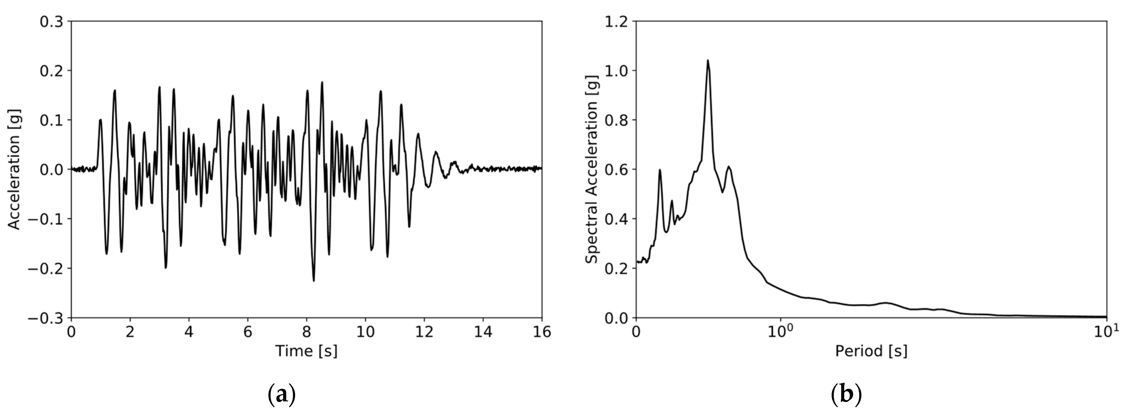
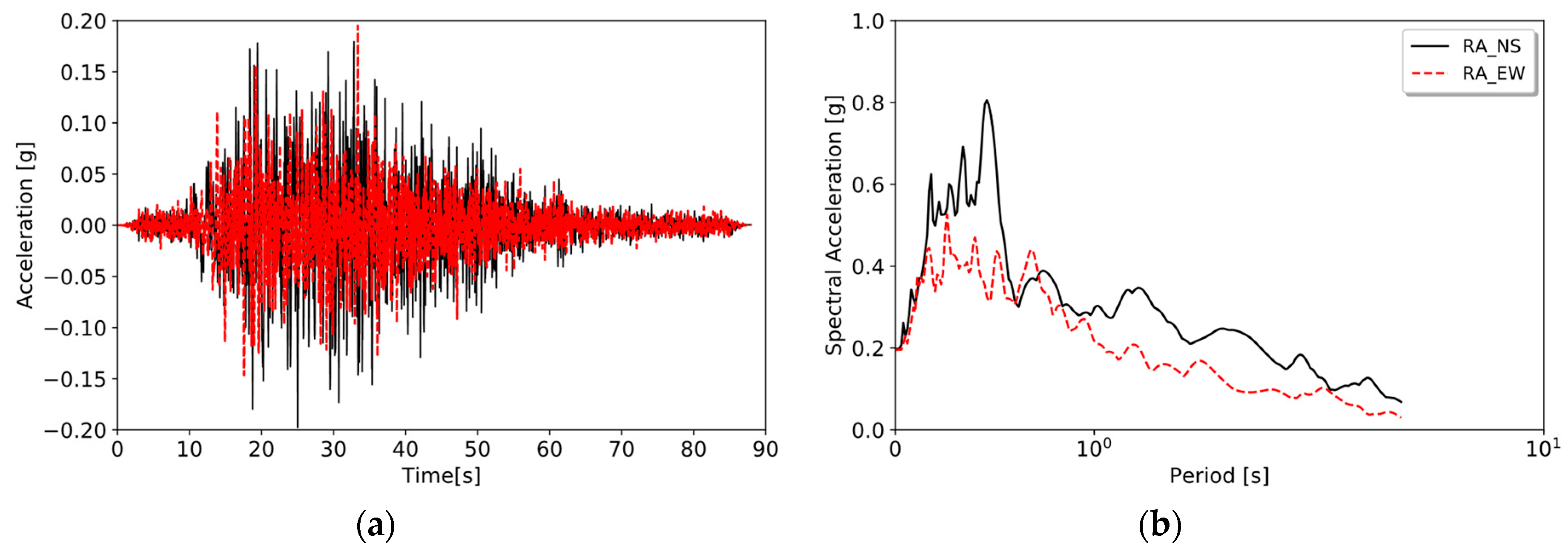
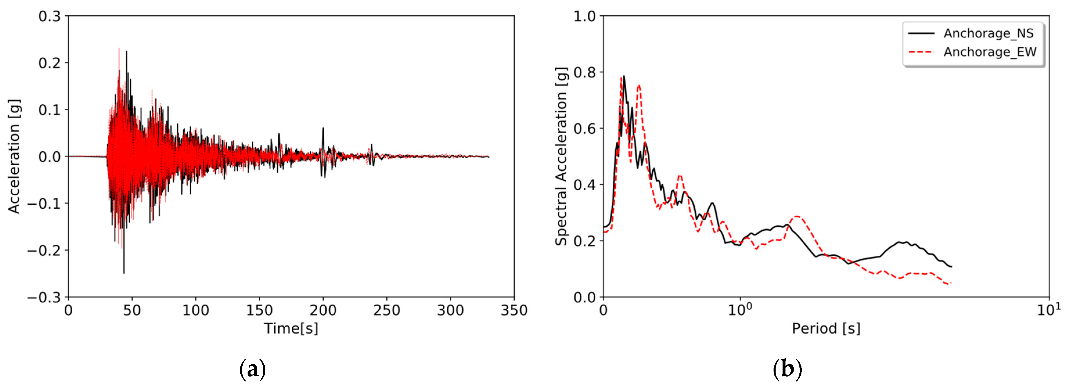
3.2.2. Model Input Ground Motion
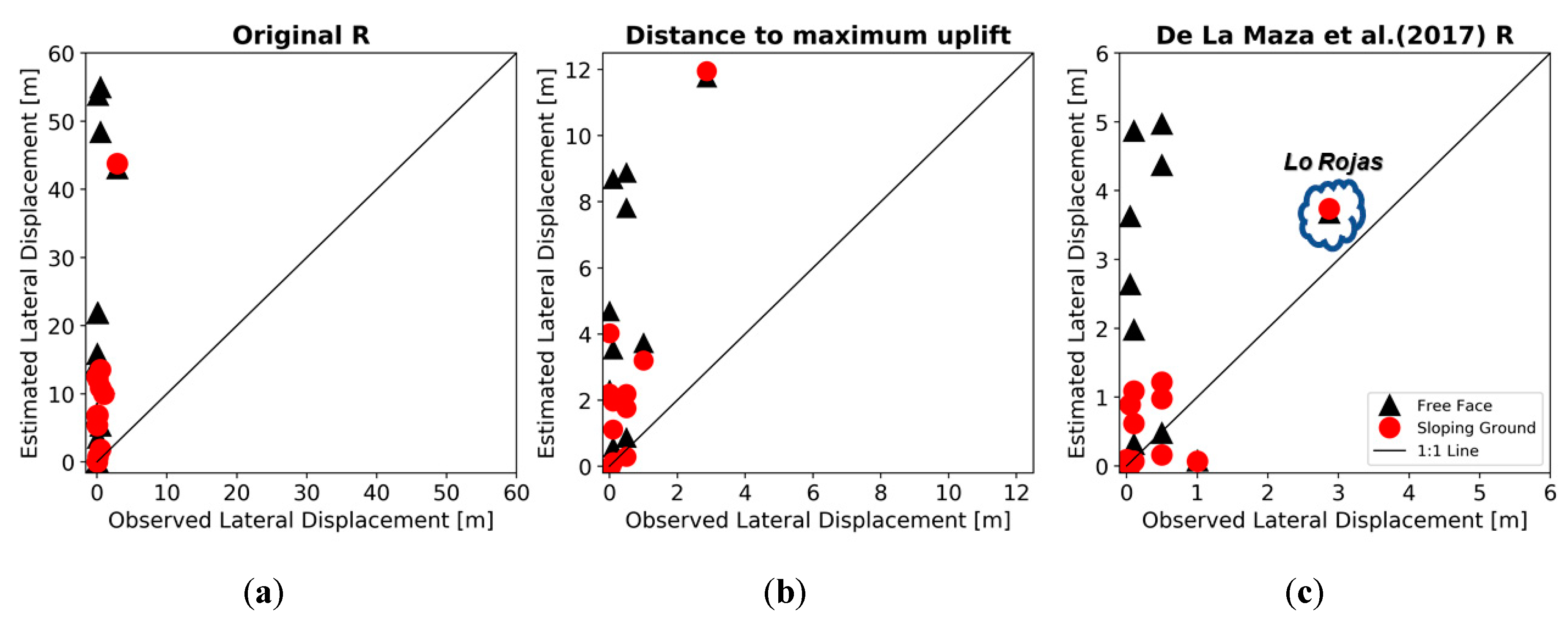
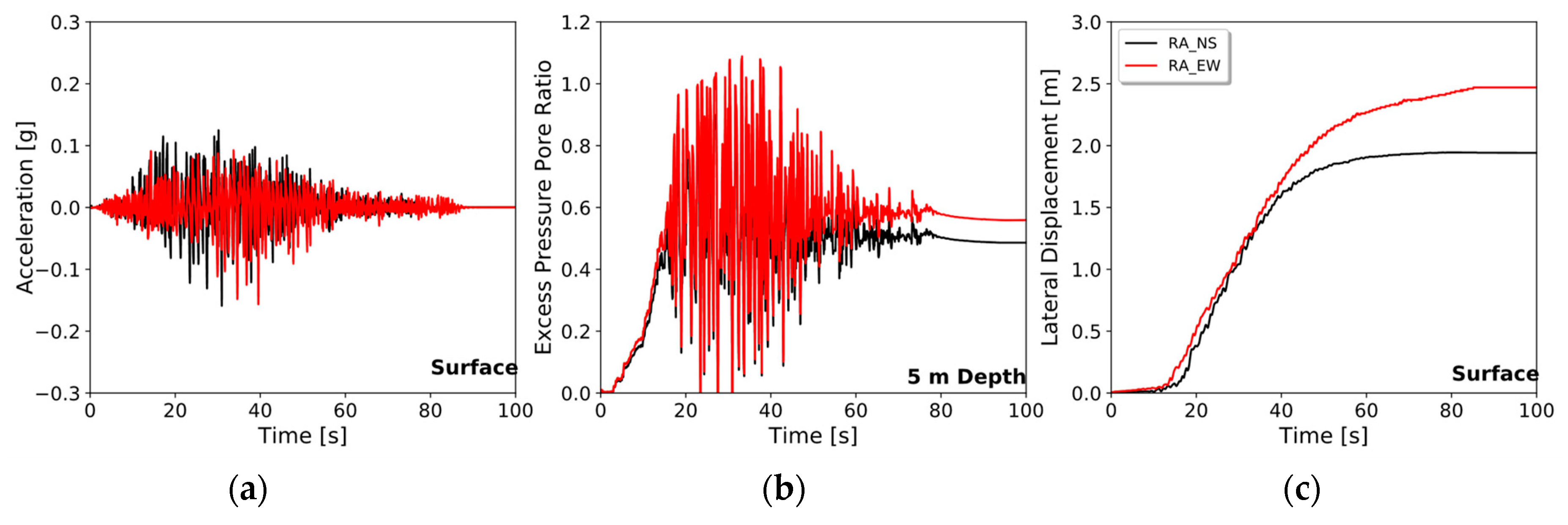
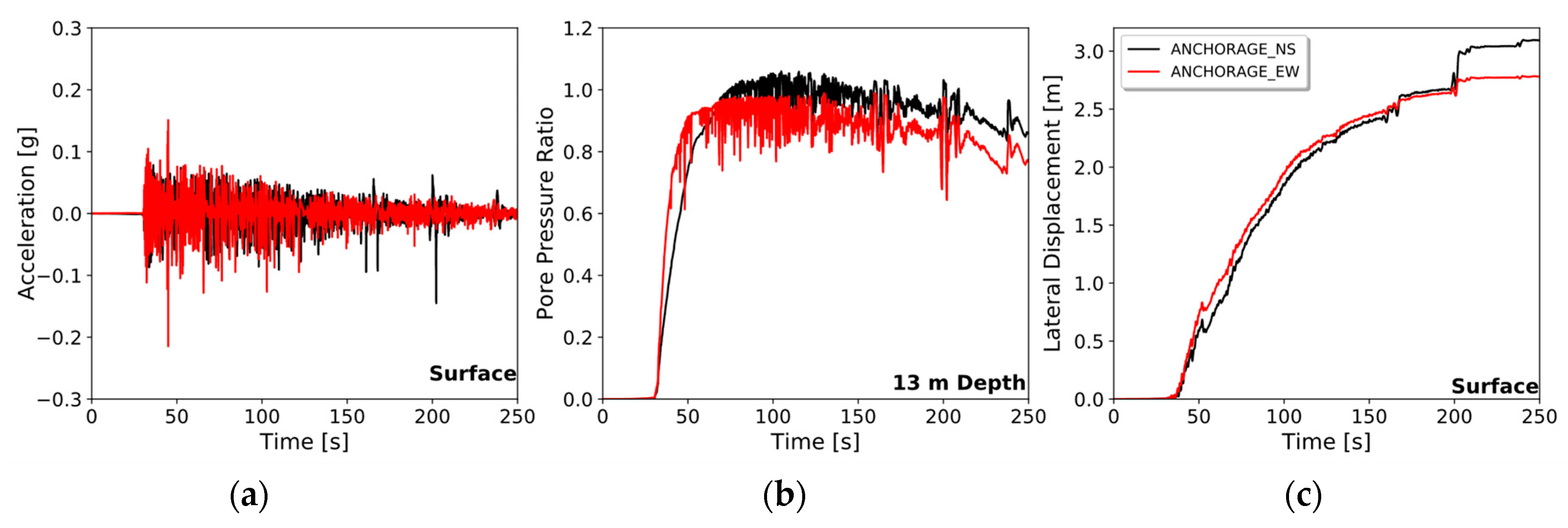
3.2.3. Simulation Results
4. Parametric study using Nonlinear Site Response Analysis
4.1. Soil Profiles and Ground Motions
4.2. Results
5. Conclusions
- (1)
- The numerical methodology used in this study (using Cyclic1D) can properly simulate pore water pressure generation and shear modulus degradation under strong earthquakes.
- (2)
- The applicability of the numerical methodology was verified by comparing the simulated responses and the recorded ones in the centrifuge tests of the VELACS and LEAP projects, and those from simulated historical cases.
- (3)
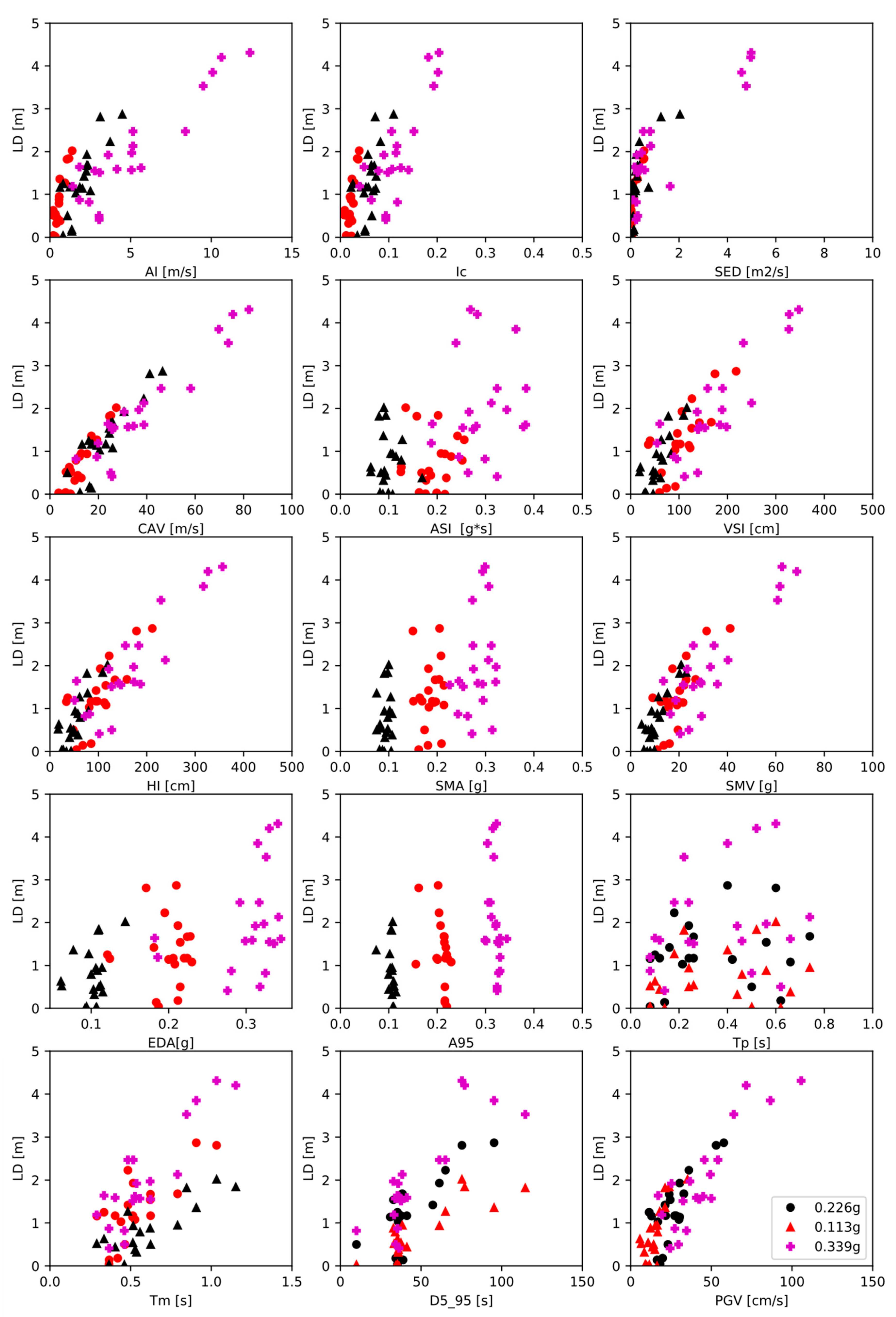
- Our parametric study shows that, for the analyzed cases, the residual lateral displacement has a better correlation with CAV = cumulative absolute velocity (R2 = 0.87, ρ = 0.93, rs = 0.88), HI = Housner intensity (R2 = 0.78, ρ = 0.88, rs = 0.79) and SMV = sustained maximum velocity (R2 = 0.78, ρ = 0.88, rs = 0.79).
- (4)
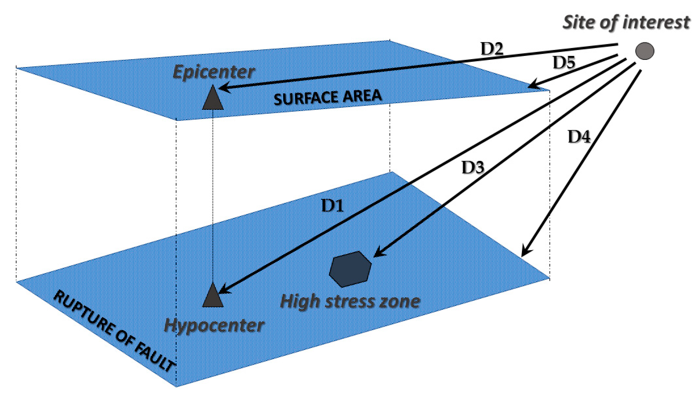
- For large-magnitude subduction earthquakes, the use of the distance terms in empirical formulas is still problematic.
- (5)
- In future stages of this research, a probabilistic approach that incorporates different sources of uncertainty in seismic loading, soil properties, and soil geometry will be developed.
Author Contributions
Funding
Acknowledgments
Conflicts of Interest
Nomenclature
| R | Distance from site to the seismic source | A95 | Threshold of acceleration when 95% of AI is achieved |
| D1 | Hypocentral distance | EPP | Excess pressure pore |
| D2 | Epicentral distance | ru | Excess pressure pore ratio |
| D3 | Closest distance to high-stress zone | SPT | Standard Penetration Test |
| D4 | Closest distance to the edge of the fault rupture | Vmax/Amax | Maximum velocity to maximum acceleration ratio |
| D5 | Closest distance to the surface projection of the rupture | Ic | Intensity characteristic |
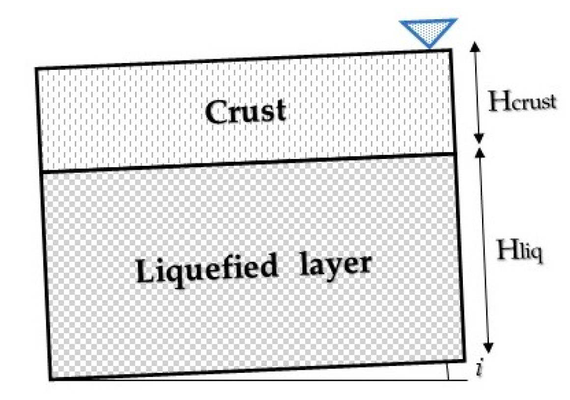
| i | Ground slope | SED | Specific energy density |
| Dr | Relative density | CAV | Cumulative absolute velocity |
| H | Liquefied Thickness | ASI | Acceleration spectrum intensity |
| amax | Maximum horizontal acceleration | VSI | Velocity spectrum intensity |
| Dh | Lateral displacement at the surface | HI | Housner intensity |
| ρ | Mass density | SMA | Sustained maximum acceleration |
| Vsr | Reference shear wave velocity | SMV | Sustained maximum velocity |
| coeff | Confinement dependence coefficient | EDA | Effective design acceleration |
| K0 | Coefficient of lateral pressure | Perm k | Permeability coefficient |
| ϕ | Friction angle | Tp | Predominant period |
| γ | Peak shear strain | Tm | Mean period |
| NYS | Number of yield surfaces | SD | Significant duration |
| PT | Phase transformation angle | UD | Uniform duration |
| c1 | Contraction parameter 1 | BD | Bracketed duration |
| c2 | Contraction parameter 2 | PGV | Peak ground velocity |
| d1 | Dilatation parameter 1 | PGD | Peak ground displacement |
| d2 | Dilatation parameter 2 | AI | Arias intensity |
| Liq | Liquefaction parameter | ARMS | Root-mean-square acceleration |
| LD | Lateral displacement at the surface in the parametric study | VRMS | Root-mean-square velocity |
| PGD | Peak ground displacement | DRMS | Root-mean-square displacement |
References
- Valsamis, A.I.; Bouckovalas, G.D.; Papadimitriou, A.G. Parametric investigation of lateral spreading of gently sloping liquefied ground. Soil Dyn. Earthq. Eng. 2010, 30, 490–508. [Google Scholar] [CrossRef]
- Bartlett, S.F.; Youd, T.L. Empirical Prediction of Liquefaction Induced Lateral Spread. J. Geotech. Eng. 1995, 121, 316–329. [Google Scholar] [CrossRef]
- Faris, A.T.; Seed, R.B.; Kayen, R.E.; Wu, J. A semi-empirical model for the estimation of maximum horizontal displacement due to liquefaction-induced lateral spreading. In Proceedings of the 8th US National Conference on Earthquake Engineering, San Francisco, CA, USA, 18–22 April 2006; Volume 3, p. 1323. [Google Scholar]
- Zhang, J.; Yang, C.; Zhao, J.X.; McVerry, G.H. Empirical models for predicting lateral spreading considering the effect of regional seismicity. Earthq. Eng. Eng. Vib. 2012, 11, 121–131. [Google Scholar] [CrossRef]
- Youd, L.T.; Hansen, C.M.; Bartlett, S.F. Revised Multilinear Regression Equations for Prediction of Lateral Spread Displacement. J. Geotech. Geoenviron. Eng. 2002, 128, 1007–1017. [Google Scholar] [CrossRef]
- Rauch, A.F.; Martin, J.R. EPOLLS Model For Prediction Average Displacements On Lateral Spreads. J. Geotech. Geoenviron. Eng. 2006, 126, 165–172. [Google Scholar]
- Tryon, G.E. Evaluation of Current Empirical Methods for Predicting Lateral Spread-Induced Ground Deformations for Large Magnitude Earthquakes Using Maule Chile 2010 Case Histories. Master’s Thesis, Brigham Young University, Provo, UT, USA, 2014. [Google Scholar]
- Williams, N.D. Evaluation of Empirical Prediction Methods for Liquefaction-Induced Lateral Spread from the 2010 Maule, Chile, Mw 8.8 Earthquake in Port Coronel. Master’s Thesis, Brigham Young University, Provo, UT, USA, 2015. [Google Scholar]
- Elgamal, A.; Yang, Z.; Parra, E. Computational modeling of cyclic mobility and post-liquefaction site response. Soil Dyn. Earthq. Eng. 2002, 22, 259–271. [Google Scholar] [CrossRef]
- Bray, J.D.; Boulanger, R.; Kramer, S.L.; Rourke, T.O.; Green, R.A.; Rob, P.K.; Beyzaei, C.Z. Liquefaction-Induced Ground Movement Effects. In Proceedings of the U.S.–New Zealand–Japan International Workshop, PEER Report 2017/02, Berkeley, CA, USA, 2–4 November 2016; p. 150. [Google Scholar]
- Kawata, Y.; Nagamatsu, S.; Koshiyama, K.; Nishimura, H.; Abe, S.; Takatorige, T.; Hayashi, Y.; Takahashi, T.; Koyama, T.; Yamasaki, E.; et al. Chapter 8—Liquefaction With the Great East Japan Earthquake. In The Fukushima and Tohoku Disaster; Elsevier Inc.: Suita, Japan, 2018; pp. 147–159. [Google Scholar]
- Youd, T.L. Application of MLR Procedure for Prediction of Liquefaction-Induced Lateral Spread Displacement. J. Geotech. Geoenvironmental Eng. 2018, 6, 144. [Google Scholar] [CrossRef]
- Jia, J. Soil Dynamics and Foundation Modeling. In Liquefaction; Springer International Publishing: Cham, Switzerland, 2017; p. 740. [Google Scholar]
- Mccrink, T.P.; Pridmore, C.L.; Tinsley, J.C.; Sickler, R.R.; Brandenberg, S.J.; Stewart, J.P. Liquefaction and Other Ground Failures in Imperial County, California, from the April 4, 2010, El Mayor—Cucapah Earthquake; United States Geological Survey: Reston, VA, USA, 2011.
- Aydan, Ö.; Miwa, S.; Komada, H.; Suzuki, T. The M8.7 Nias Earthquake of March 28, 2005; Tokai University: Shizuka, Japan, 2005. [Google Scholar]
- Hamada, M.; Towhata, I.; Yasuda, S.; Isoyama, R. Study on permanent ground displacement induced by seismic liquefaction. Comput. Geotech. 1987, 4, 197–220. [Google Scholar] [CrossRef]
- Zhang, G.; Robertson, P.; Brachman, R. Estimating Liquefaction-Induced Lateral Displacements Using the Standard Penetration Test or Cone Penetration Test. J. Geotech. Geoenviron. Eng. 2004, 130, 861–871. [Google Scholar] [CrossRef]
- Olson, S.M.; Johnson, C.I. Analyzing Liquefaction-Induced Lateral Spreads Using Strength Ratios. J. Geotech. Geoenviron. Eng. 2008, 134, 1035–1049. [Google Scholar] [CrossRef]
- Gillins, D.T.; Bartlett, S.F. Multilinear regression equations for predicting lateral spread displacement from soil type and cone penetration test data. J. Geotech. Geoenviron. Eng. 2014, 140, 1–11. [Google Scholar] [CrossRef]
- Pirhadi, N.; Tang, X.; Yang, Q. New Equations to Evaluate Lateral Displacement Caused by Liquefaction Using the Response Surface Method. J. Mar. Sci. Eng. 2019, 7, 35. [Google Scholar] [CrossRef]
- Joyner, W.; Boore, D.M. Measurement, characterization, and prediction of strong ground motion. Geotech. Spec. Publ. 1988, 43–102. [Google Scholar]
- De la Maza, G.; Williams, N.; Sáez, E.; Ledezma, C. Liquefaction-Induced Lateral Spread in Lo Rojas, Coronel, Chile: Field Study and Numerical Modeling. Earthq. Spectra 2017, 33, 219–240. [Google Scholar] [CrossRef]
- Moreno, M.; Rosenau, M.; Oncken, O. 2010 Maule earthquake slip correlates with pre-seismic locking of Andean subduction zone. Nature 2010, 467, 198–202. [Google Scholar] [CrossRef]
- Yang, Z.; Elgamal, A.; Parra, E. Computational model for cyclic mobility and associated shear deformation. J. Geotech. Geoenviron. Eng. 2003, 129, 1119–1127. [Google Scholar] [CrossRef]
- Elgamal, A.; Yang, Z.; Parra, E.; Ragheb, A. Modeling of cyclic mobility in saturated cohesionless soils. Int. J. Plast. 2003, 19, 883–905. [Google Scholar] [CrossRef]
- Elgamal, A.; Yang, Z.; Lu, J. Cyclic1D User’s Manual; University of California: San Diego, CA, USA, 2015. [Google Scholar]
- Taboada, V.M.; Dobry, R. Centrifuge modeling of earthquake-induced lateral spreading in sand. J. Geotech. Geoenviron. Eng. 1998, 124, 1195–1206. [Google Scholar] [CrossRef]
- Sharp, M.K.; Dobry, R.; Abdoun, T. Liquefaction centrifuge modeling of sands of different permeability. J. Geotech. Geoenviron. Eng. 2003, 129, 1083–1091. [Google Scholar] [CrossRef]
- Ziotopoulou, K. Seismic response of liquefiable sloping ground: Class A and C numerical predictions of centrifuge model responses. Soil Dyn. Earthq. Eng. 2018, 113, 744–757. [Google Scholar] [CrossRef]
- Mercado, V.; Ochoa-Cornejo, F.; Astroza, R.; El-Sekelly, W.; Abdoun, T.; Pastén, C.; Hernández, F. Uncertainty quantification and propagation in the modeling of liquefiable sands. Soil Dyn. Earthq. Eng. 2019, 123, 217–229. [Google Scholar]
- Phoon, M.; Kulhawy, K.; Grigoriu, F.H. Statistical Guidelines For Soil Property Evaluation. In Reliability-Based Design of Foundations for Transmission Line Structures; Electronic Power Research Institute: Buffalo, CA, USA, 1995; p. 384. [Google Scholar]
- Arulanandan, K.; Scott, R.F. Project VELACS-Control Test Results. J. Geotech. Eng. 1994, 119, 1276–1292. [Google Scholar]
- Kutter, B.L.; Carey, T.J.; Hashimoto, T.; Zeghal, M.; Abdoun, T.; Kokkali, P.; Madabhushi, G.; Haigh, S.K.; Burali d’Arezzo, F.; Madabhushi, S.; et al. LEAP-GWU-2015 experiment specifications, results, and comparisons. Soil Dyn. Earthq. Eng. 2018, 113, 616–628. [Google Scholar]
- Carey, T.J.; Kutter, B.L.; Manzari, M.T.; Zeghal, M. Leap Soil Properties and Element Test Data. Available online: https://datacenterhub.org/resources/14316 (accessed on 26 May 2020).
- Parra, B.A.; Boulanger, R.W.; Carey, T.; DeJong, J. Ottawa F-65 Sand Data from Ana Maria Parra Bastidas. Available online: https://datacenterhub.org/resources/ottawa_f_65 (accessed on 26 May 2020).
- Arulmoli, K.; Muraleetharan, K.K.; Hossain, M.M.; Fruth, L.S. VELACS: Verifications of Liquefaction Analyses by Centrifuge Studies. Laboratory Testing Program. Soil Data Report; Earth Technology Corporation: Irvine, CA, USA, 1992. [Google Scholar]
- Jaky, J. The coefficient of earth pressure at rest. J. Soc. Hung. Archit. Eng. 1944, 78, 355–388. [Google Scholar]
- Seed, H.B.; Idriss, I. Evaluation of liquefaction potential sand deposits based on observation of performance in previous earthquakes. ASCE Natl. Conv. 1981, 81–544. [Google Scholar]
- Darendeli, M. Development of a New Family of Normalized Modulus Reduction and Material Damping Curves; University of Texas at Austin: Austin, TX, USA, 2001. [Google Scholar]
- Mavroeidis, G.P.; Zhang, B.; Dong, G.; Papageorgiou, A.S.; Dutta, U.; Biswas, N.N. Estimation of strong ground motion from the great 1964 Mw 9.2 Prince William Sound, Alaska, earthquake. Bull. Seismol. Soc. Am. 2008, 98, 2303–2324. [Google Scholar] [CrossRef]
- Barrueto, C.; Sáez, E.; Ledezma, C. Seismic demand on piles in sites prone to liquefaction-induced lateral spreading. In Proceedings of the 16th World Conference on Earthquake, 16WCEE 2017, Santiago, Chile, 9–13 January 2017. [Google Scholar]
- Bartlett, S.F.; Youd, T.L. Empirical Analysis of Horizontal Ground Displacement Generated by Liquefaction- Induced Lateral Spreads by Liquefaction- Induced Lateral Spreads; National Center For Earthquake Engineering Research: Buffalo, NY, USA, 1992. [Google Scholar]
- Wu, J.; Kammerer, A.M.; Riemer, M.F.; Seed, R.B.; Pestana, J.M. Labory study of liquefaction triggering criteria. In Proceedings of the 13th World Conference on Earthquake Engineering, Berkeley, CA, USA, 1–6 August 2004; p. 14. [Google Scholar]
- Mayne, P.W. In-Situ Test Calibrations for Evaluating Soil Parameters; Geosystems Engineering Group: Singapore, 2016. [Google Scholar]
- Bray, J.; Rollins, K.; Hutchinson, T.; Verdugo, R.; Ledezma, C.; Mylonakis, G.; Assimaki, D.; Montalva, G.; Arduino, P.; Olson, S.M.; et al. Effects of ground failure on buildings, ports, and industrial facilities. Earthq. Spectra 2012, 28, 97–118. [Google Scholar]
- Ledezma, C.; Hutchinson, T.; Ashford, S.A.; Moss, R.; Arduino, P.; Bray, J.D.; Olson, S.; Hashash, Y.M.; Verdugo, R.; Frost, D.; et al. Effects of ground failure on bridges, roads, and railroads. Earthq. Spectra 2012, 28, 119–143. [Google Scholar]
- Pollitz, F.F.; Brooks, B.; Tong, X.; Bevis, M.G.; Foster, J.H.; Bürgmann, R.; Smalley, R.; Vigny, C.; Socquet, A.; Ruegg, J.-C.; et al. Coseismic slip distribution of the February 27, 2010 Mw 8.8 Maule, Chile earthquake. Geophys. Res. Lett. 2011, 38, 1–5. [Google Scholar]
- Rauch, A.F. EPOLLS: An Empirical Method for Predicting Surface Displacements Due to Liquefaction-Induced Lateral Spreading in Earthquakes. Ph.D. Thesis, Virginia Polytechnic Institute, Blacksburg, VA, USA, 1997. [Google Scholar]


| Author(s) | Variables |
|---|---|
| Hamada et al. (1987) [16] | Ground slope, thickness of the liquefiable layer |
| Bartlett and Youd (1995) [2] | Ground slope, thickness of the liquefiable layer, fines content, average grain size, earthquake magnitude, horizontal distance from the site to the seismic energy source. |
| Youd et al. (2002) [5] | Ground slope, thickness of the liquefiable layer, fines content, average grain size, earthquake magnitude, horizontal distance from the site to the seismic energy source. |
| Zhang et al. (2004) [17] | Ground slope, thickness of the liquefiable layer, shear strain, earthquake magnitude, depth to the liquefiable layer. |
| Faris et al. (2006) [3] | Seismic coefficient, earthquake magnitude, horizontal distance from the site to the seismic energy source. |
| Olson and Jhonson (2008) [18] | Ground slope, thickness of the liquefiable layer, fines content, average grain size, earthquake magnitude, horizontal distance from the site to the seismic energy source, post-liquefaction undrained shear strength. |
| Zhang et al. (2012) [4] | Ground slope, thickness of the liquefiable layer, fines content, average grain size, pseudo-spectral displacement. |
| Gillins and Bartlett (2014) [19] | Ground slope, thickness of the liquefiable layer, fines content, average grain size, earthquake magnitude, horizontal distance from the site to the seismic energy source. |
| Pirhadi et al. (2019) [20] | Ground slope, thickness of the liquefiable layer, fines content, average grain size, earthquake magnitude, cumulative absolute velocity, peak ground acceleration. |
| Test | i [°] | Dr [%] | H [m] | amax [g] | Dh [cm] | Reference |
|---|---|---|---|---|---|---|
| M1-2 | 0 | 40–45 | 10 | 0.23 | 1.7 | Taboada and Dobry (1998) [27] |
| M2-2 | 1.94 | 40–45 | 10 | 0.23 | 47.0 | Taboada and Dobry (1998) [27] |
| M2c-6 | 3.95 | 40–45 | 10 | 0.17 | 72.5 | Taboada and Dobry (1998) [27] |
| L45V2-10 | 2 | 45 | 10 | 0.23 | 66 | Sharp et al. (2003) [28] |
| L65V2-10 | 2 | 65 | 10 | 0.20 | 28 | Sharp et al. (2003) [28] |
| L75V2-10 | 2 | 75 | 10 | 0.21 | 23 | Sharp et al. (2003) [28] |
| RPI-02 | 5 | 65 | 5 | 0.17 | 35 | Ziotopoulou (2018) [29] |
| Parameter | Nevada Sand Dr = 40% | Ottawa F65 Dr = 65% | Mean Value 1 | Standard Deviation 1 | Coefficient of Variation 1 [%] |
|---|---|---|---|---|---|
| Mass density [ρ] (kg/m3) | 1800 | 1900 | 1570 | 270 | 9% |
| Reference shear wave velocity [Vs ref] (m/s) | 203.3 | 203.3 | 242.5 | 16.5 | 28% |
| Confinement coefficient [coeff] | 0.5 | 0.5 | |||
| Coefficient of lateral pressure [Ko] | 0.5 | 0.67 | |||
| Friction angle [ϕ] (°) | 31.4 | 31.4 | 40.5 | 2.1 | 5% |
| Peak shear strain [γ max] (%) | 5 | 5 | |||
| Number of yield surfaces [NYS] | 20 | 20 | |||
| Phase transformation angle [PT angle] (°) | 26.5 | 26.5 | 32.9 | 2.2 | 7% |
| Contraction parameter 1 [c1] | 0.19 | 0.19 | 0.12 | 0.04 | 32% |
| Contraction parameter 2 [c2] | 0.2 | 0.2 | |||
| Dilatation parameter 1 [d1] | 0.2 | 0.2 | 0.11 | 0.04 | 42% |
| Dilatation parameter 2 [d2] | 10 | 10 | |||
| Liquefaction parameter [Liq] | 0.015 | 0.015 | |||
| Permeability coefficient [Perm k] (m/s) | 3.3 × 10⁻³ | 6.6 × 10⁻⁵ |
| Property | Value |
|---|---|
| Specific gravity | 2.68 |
| Maximum dry density | 17.33 kN/m3 |
| Minimum dry density | 13.87 kN/m3 |
| Maximum void ratio | 0.894 |
| Minimum void ratio | 0.516 |
| D50 | 0.15 mm |
| Hydraulic conductivity | 0.0021 cm/s |
| Property | Value |
|---|---|
| Specific gravity | 2.665 |
| Maximum dry density | 1736 kg/m3 |
| Minimum dry density | 1515 kg/m3 |
| D10 | 0.133 mm |
| D50 | 0.173 mm |
| D60 | 0.215 mm |
| Hydraulic conductivity | 0.016 cm/s |
| Unit [USCS] | Depth [m] | ρ [kN/m3] | Vs [m/s] | coeff | k0 | ϕ [°] | PT [°] | Su [kPa] | K [m/s] | NYS |
|---|---|---|---|---|---|---|---|---|---|---|
| SP | 0–10 | 16 | 203 | 0.50 | 0.50 | 31.4 | 26.5 | - | 3.3 × 10⁻⁵ | 25 |
| SC | 10–20 | 20 | 224 | 0.50 | 0.65 | 35 | 26.5 | - | 6.6 × 10⁻⁵ | 20 |
| CH | 20–35 | 20 | 224 | 0 | 0.65 | - | - | 75 | 1.0 × 10⁻⁷ | 20 |
| CL | 35–70 | 21 | 254 | 0 | 0.65 | - | - | 150 | 1.0 × 10⁻⁷ | 20 |
| Unit [USCS] | Depth [m] | ρ [kN/m3] | Vs [m/s] | coeff | k0 | ϕ [°] | PT [°] | Su [kPa] | K [m/s] | NYS |
|---|---|---|---|---|---|---|---|---|---|---|
| SM | 0–6 | 20 | 203 | 0.50 | 0.50 | 31.6 | 26.5 | - | 1.2 × 10⁻³ | 20 |
| GP | 6–9 | 20 | 204 | 0.50 | 0.67 | 31.4 | 26.5 | - | 1.0 × 10⁻⁷ | 20 |
| SM | 9–17 | 20 | 204 | 0.50 | 0.67 | 31.4 | 24 | - | 6.6 × 10⁻⁵ | 20 |
| SP | 17–25 | 20 | 224 | 0.50 | 0.67 | 31.4 | 22 | - | 6.6 × 10⁻⁵ | 20 |
| CL | 25–70 | 21 | 300 | 0 | 0.67 | - | - | 75 | 1.0 × 10⁻⁹ | 20 |
| Historical Case | Maximum Measured Displacement | Maximum Simulated Displacement | Measured/Simulated Ratio |
|---|---|---|---|
| Lo Rojas | 2.85 m | 2.44 | 1.20 |
| Matanuska | 2.50 m | 3.10 | 1.30 |
| Intensity Measures (IM) | R2 | ρ | rs |
|---|---|---|---|
| Cumulative absolute velocity (CAV) | 0.87 | 0.93 | 0.88 |
| Housner intensity (HI) | 0.78 | 0.88 | 0.79 |
| Sustained maximum velocity (SMV) | 0.78 | 0.88 | 0.79 |
| Peak ground velocity (PGV) | 0.77 | 0.88 | 0.78 |
| Velocity spectrum intensity (VSI) | 0.76 | 0.87 | 0.78 |
| Arias intensity (AI) | 0.73 | 0.85 | 0.77 |
| Specific energy density (SED) | 0.66 | 0.81 | 0.85 |
| Intensity characteristic (Ic) | 0.58 | 0.78 | 0.62 |
| Uniform duration (UD) | 0.55 | 0.76 | 0.72 |
| Room-mean square velocity (VRMS) | 0.48 | 0.46 | 0.48 |
| Significant duration (D5_95) | 0.48 | 0.69 | 0.60 |
| Mean period (Tm) | 0.47 | 0.68 | 0.60 |
| Bracketed duration (BD) | 0.30 | 0.55 | 0.69 |
| Effective design acceleration (EDA) | 0.29 | 0.54 | 0.53 |
| Sustained maximum acceleration (SMA) | 0.25 | 0.50 | 0.44 |
| Acceleration spectrum intensity (ASI) | 0.21 | 0.70 | 0.50 |
| Room-mean square acceleration (ARMS) | 0.21 | 0.46 | 0.63 |
| Parameter A95 (A95) | 0.03 | 0.18 | 0.34 |
| Predominant period (Tp) | 0.01 | −0.05 | 0.17 |
| Room-mean square displacement (DRMS) | 0.01 | −0.02 | 0.06 |
© 2020 by the authors. Licensee MDPI, Basel, Switzerland. This article is an open access article distributed under the terms and conditions of the Creative Commons Attribution (CC BY) license (http://creativecommons.org/licenses/by/4.0/).
Share and Cite
Araujo, W.; Ledezma, C. Factors That Affect Liquefaction-Induced Lateral Spreading in Large Subduction Earthquakes. Appl. Sci. 2020, 10, 6503. https://doi.org/10.3390/app10186503
Araujo W, Ledezma C. Factors That Affect Liquefaction-Induced Lateral Spreading in Large Subduction Earthquakes. Applied Sciences. 2020; 10(18):6503. https://doi.org/10.3390/app10186503
Chicago/Turabian StyleAraujo, William, and Christian Ledezma. 2020. "Factors That Affect Liquefaction-Induced Lateral Spreading in Large Subduction Earthquakes" Applied Sciences 10, no. 18: 6503. https://doi.org/10.3390/app10186503
APA StyleAraujo, W., & Ledezma, C. (2020). Factors That Affect Liquefaction-Induced Lateral Spreading in Large Subduction Earthquakes. Applied Sciences, 10(18), 6503. https://doi.org/10.3390/app10186503