A Vision-Based Two-Stage Framework for Inferring Physical Properties of the Terrain


Abstract
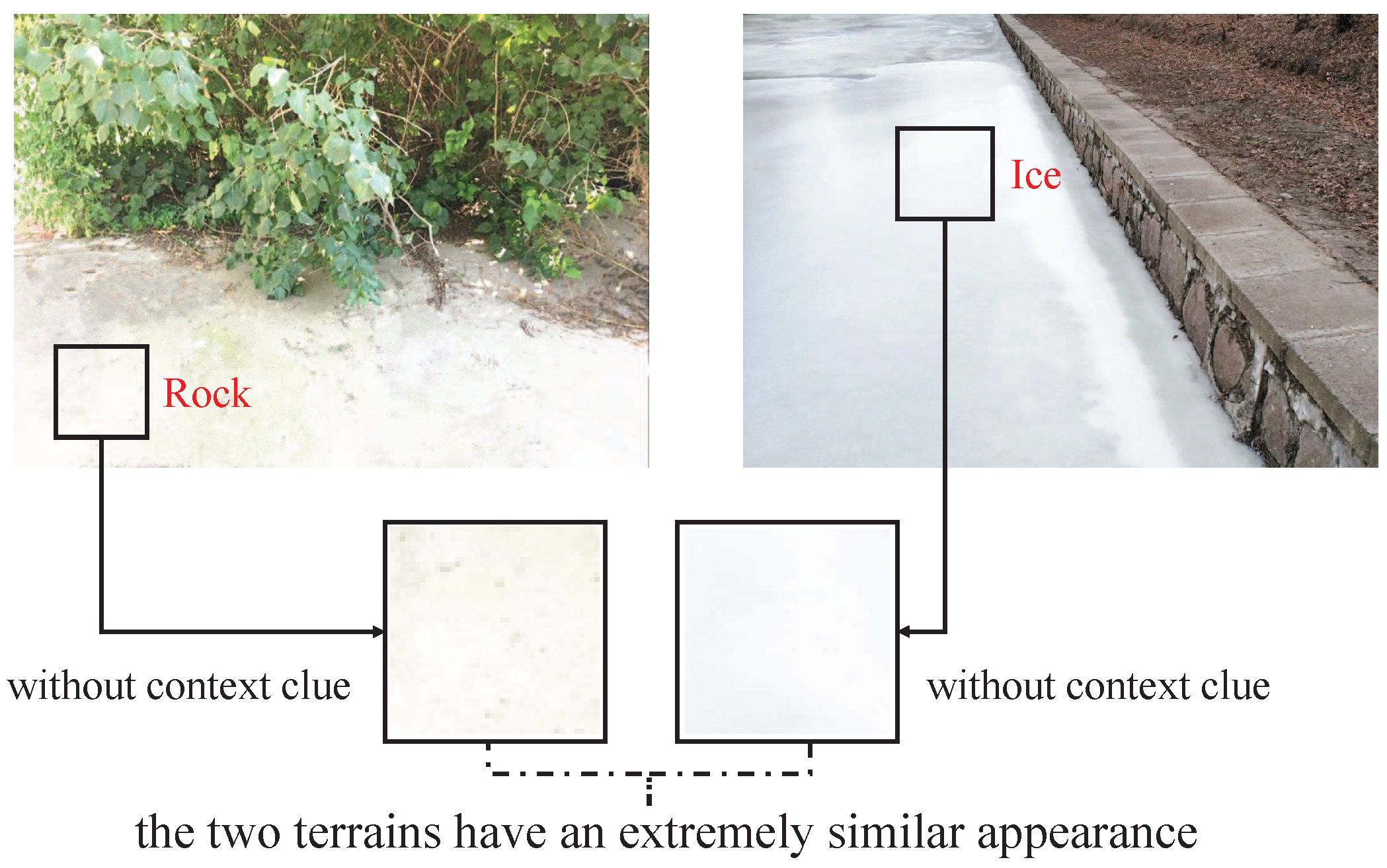
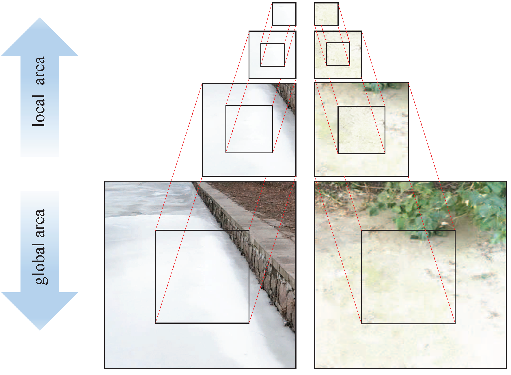
1. Introduction
2. Proposed Method
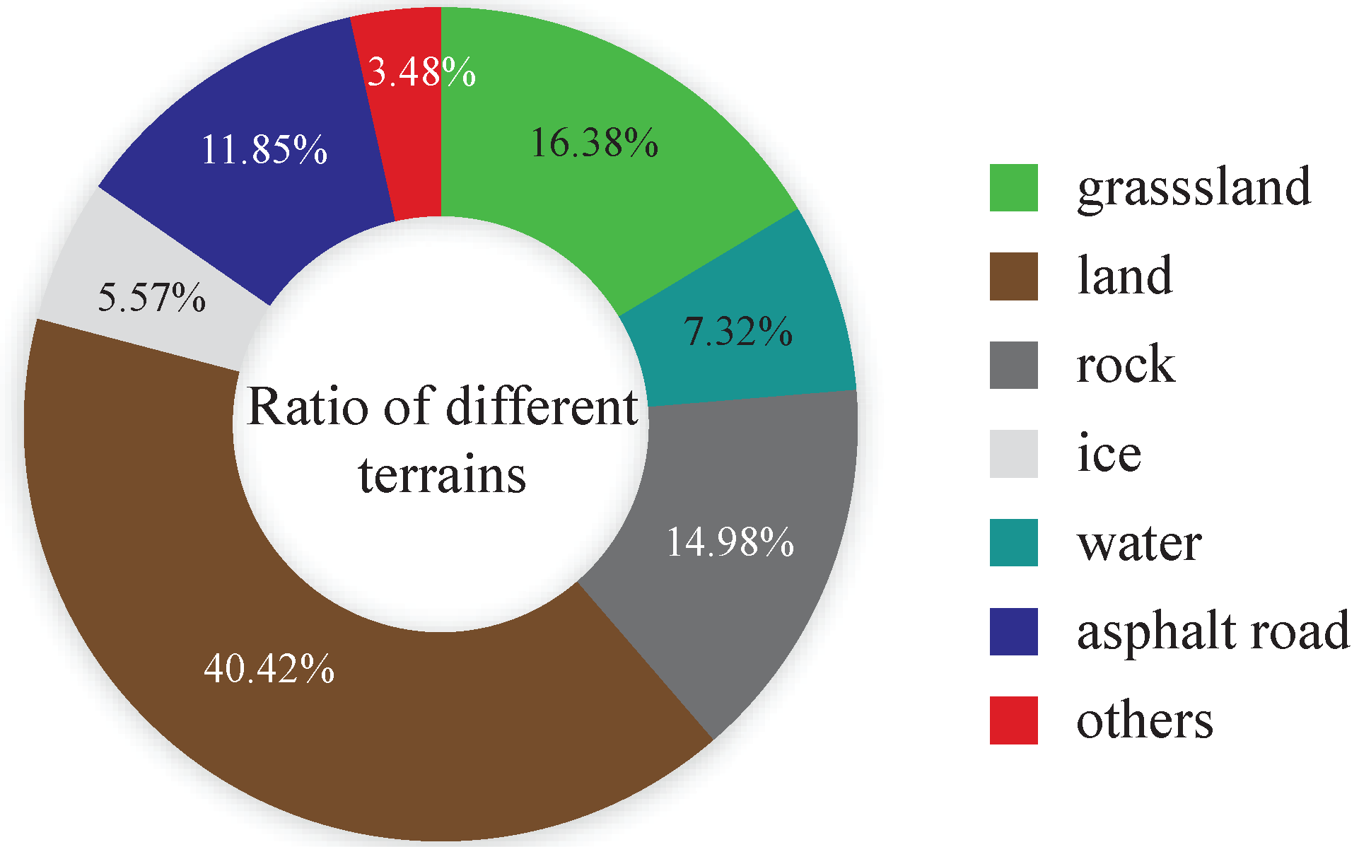
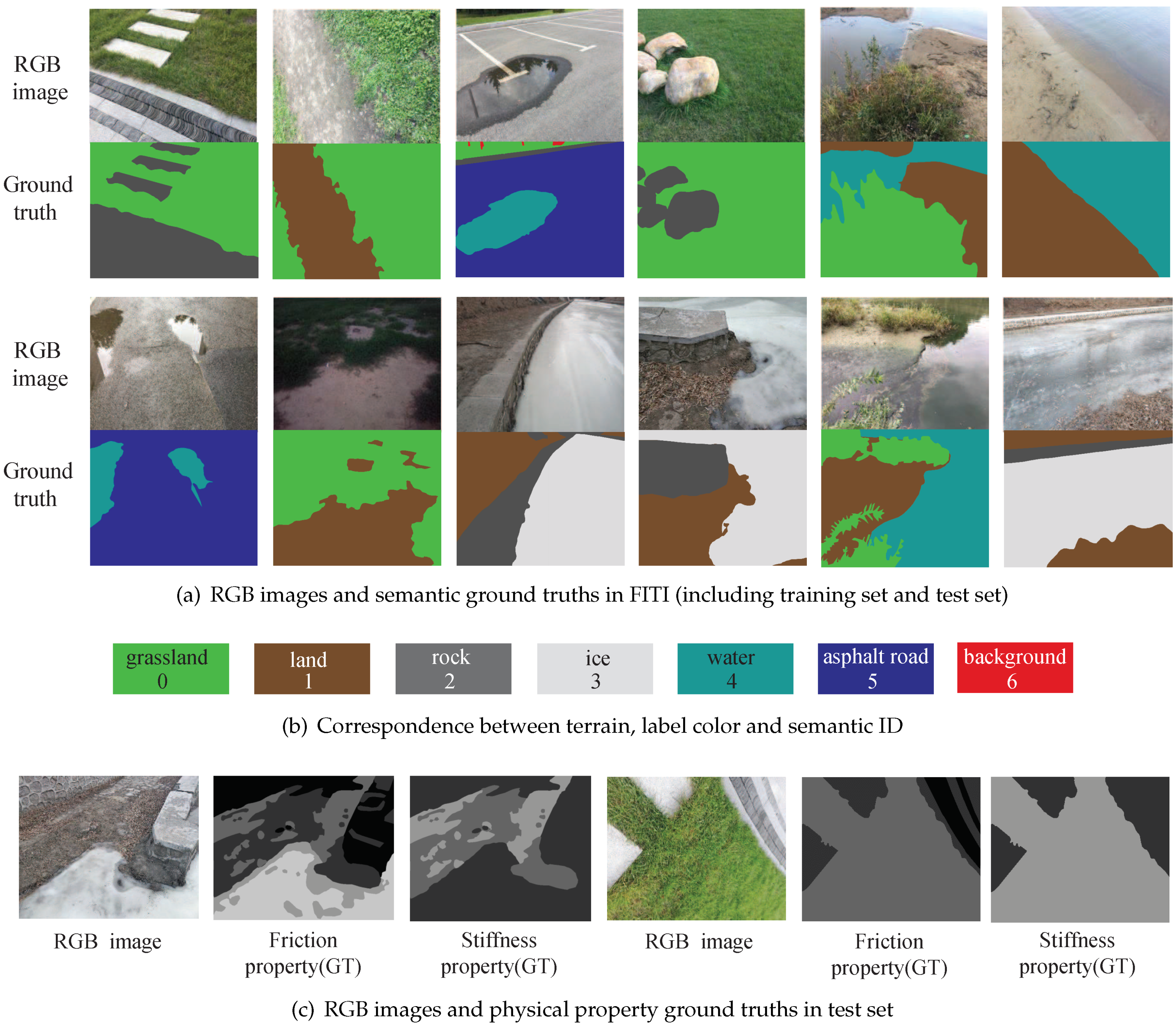
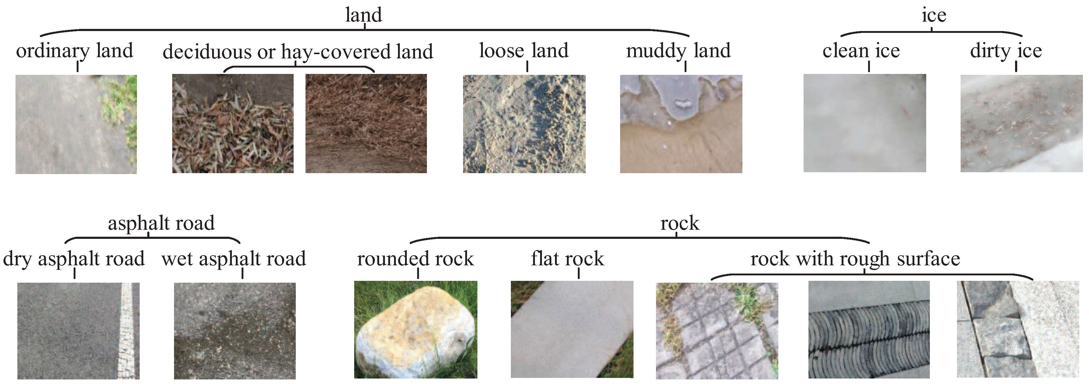
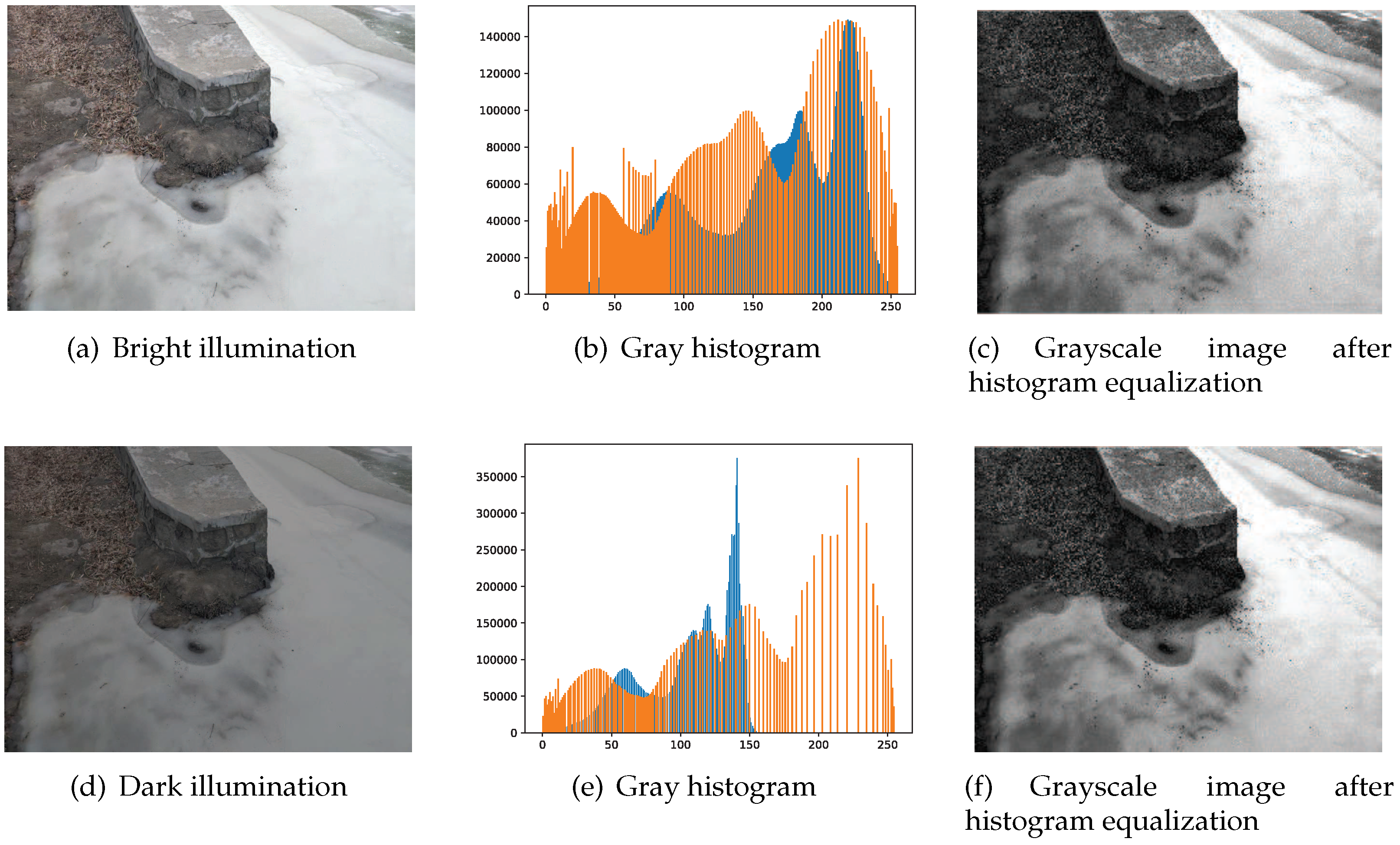
2.1. FITI Dataset
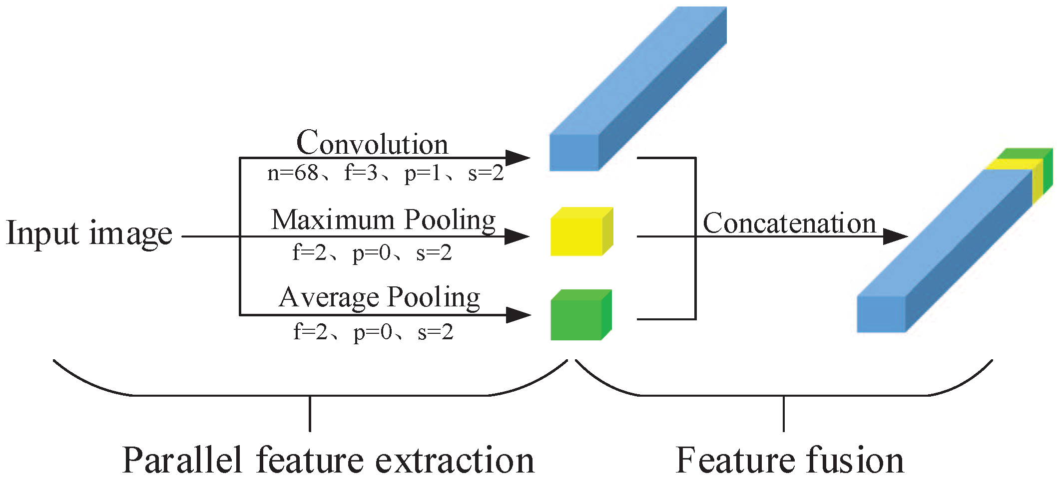
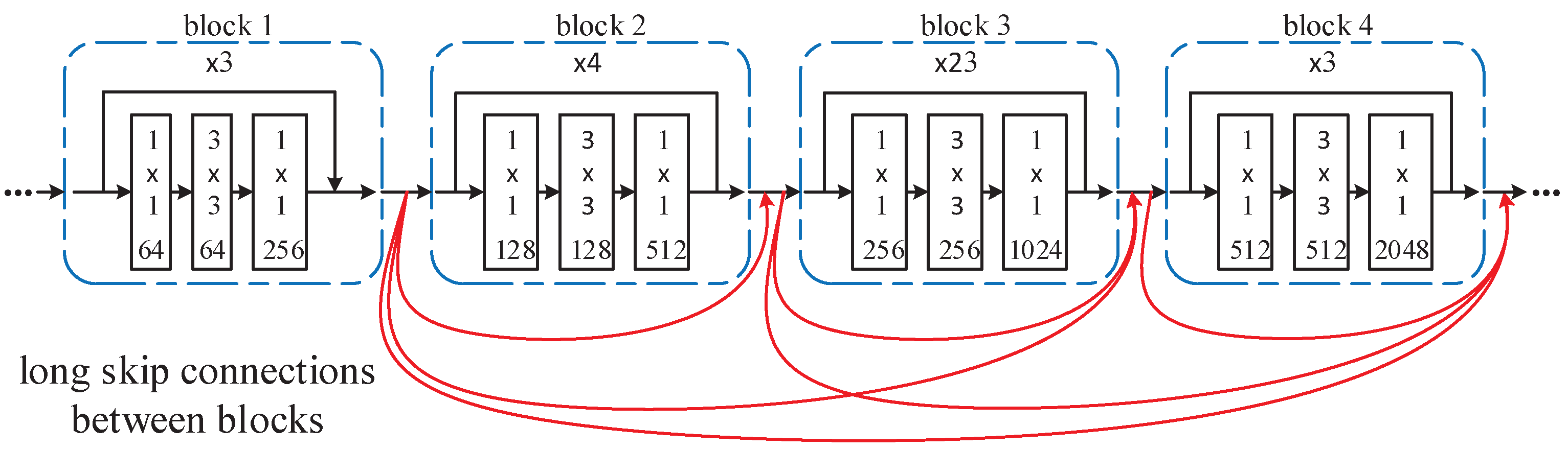
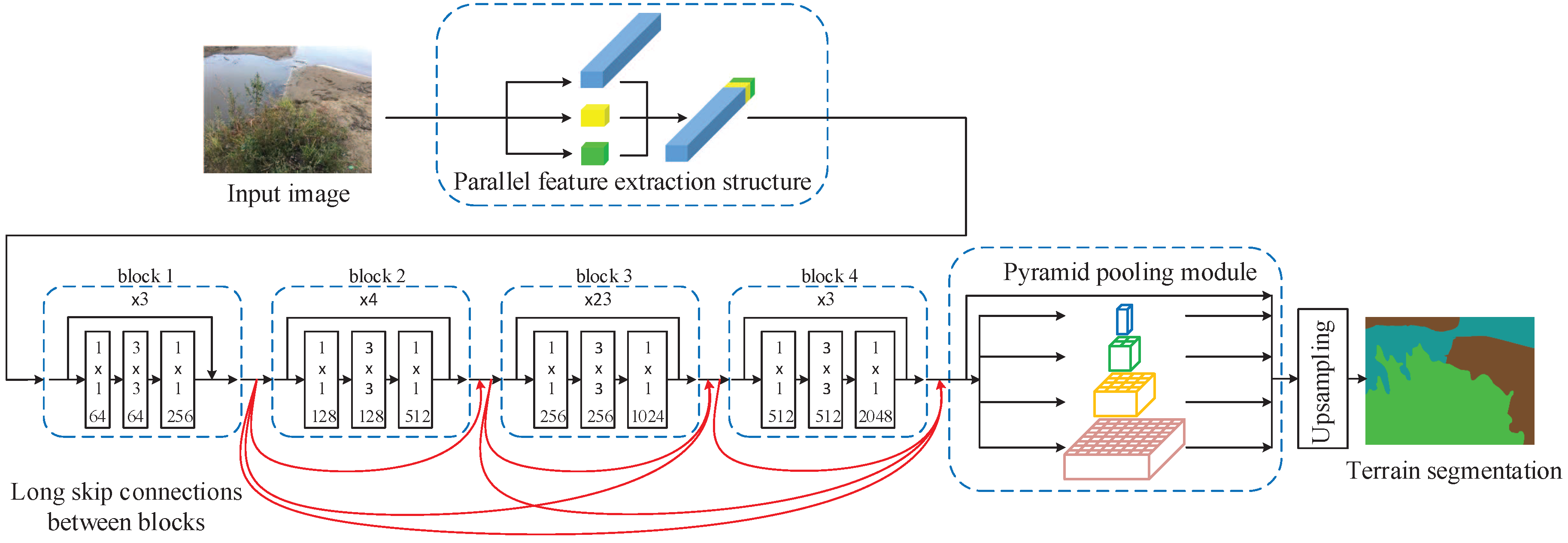
2.2. First Stage: From RGB Image to the Terrain Type
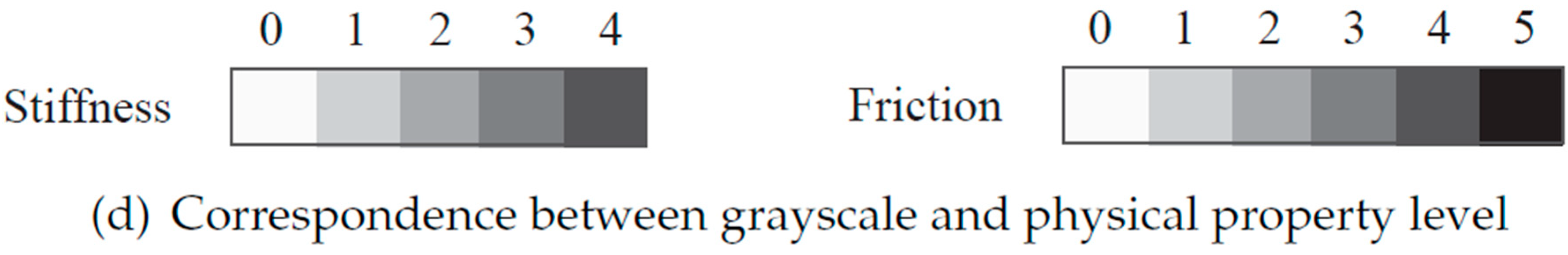
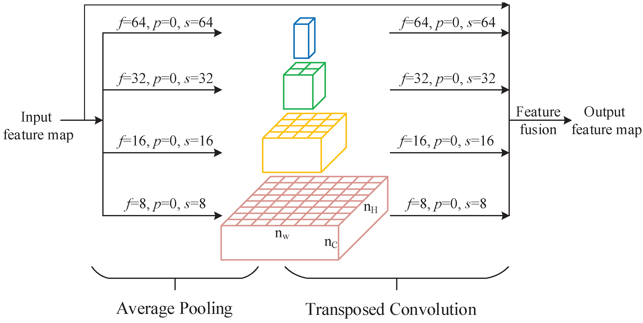
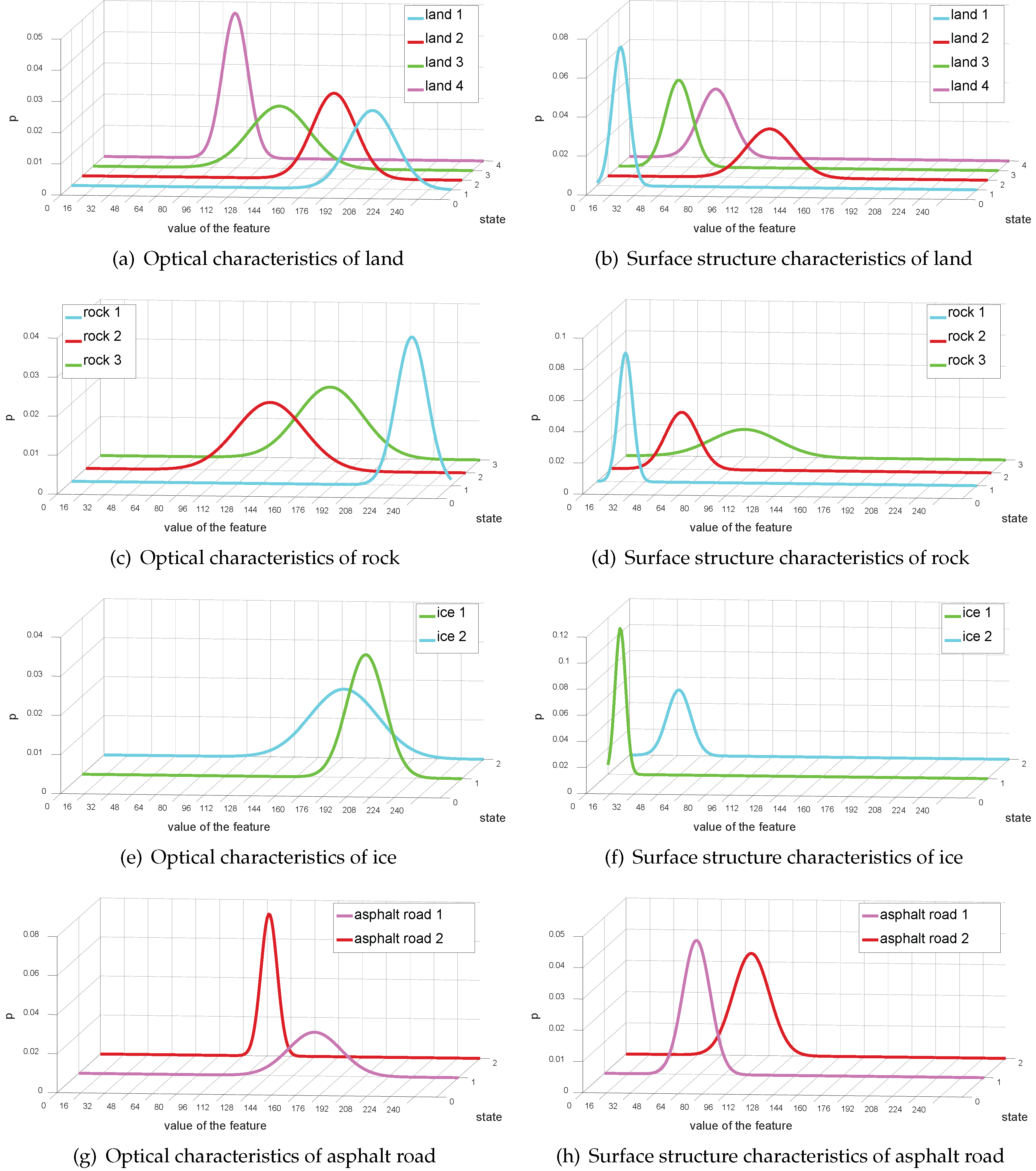
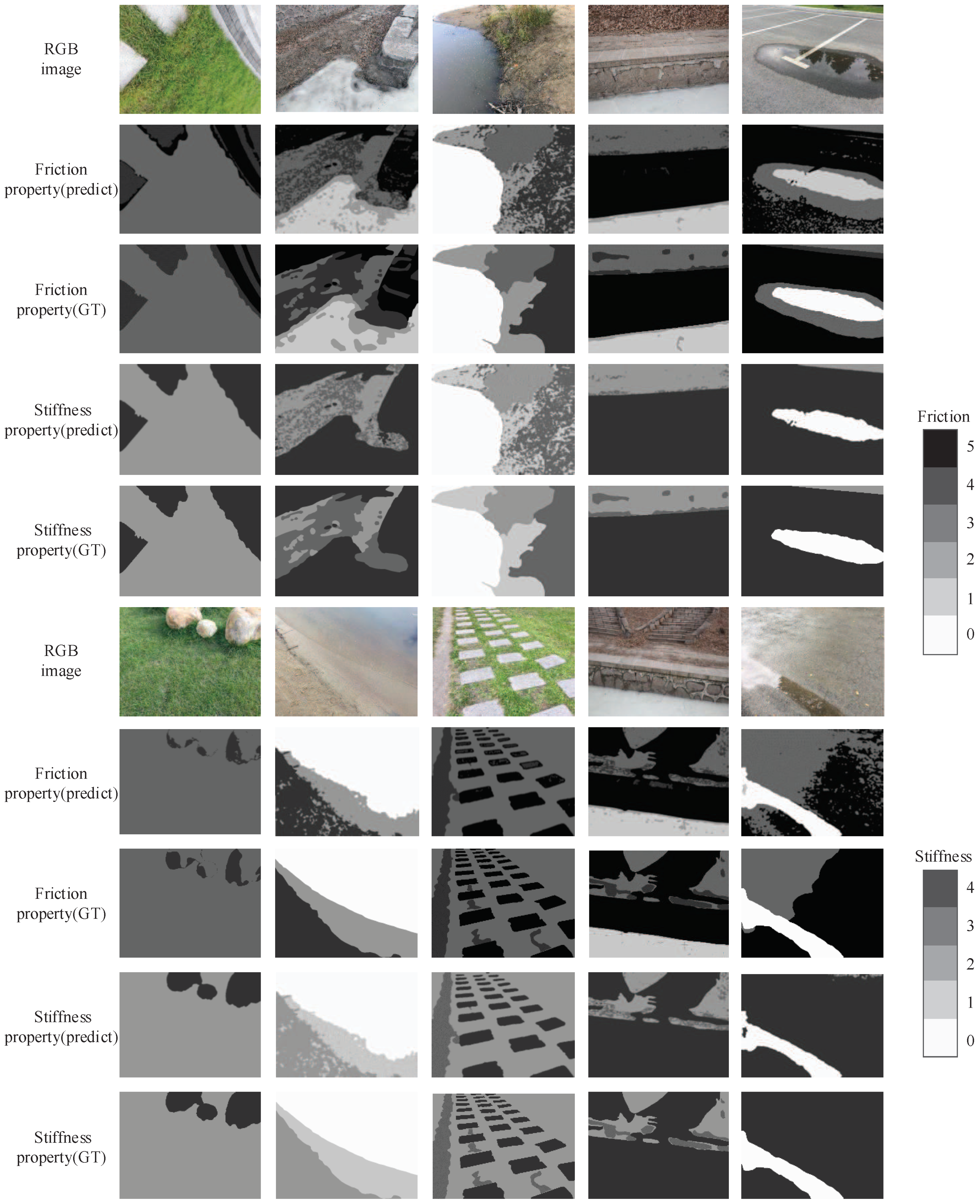
2.3. Second Stage: From the Terrain Type to Physical Properties
3. Experiment
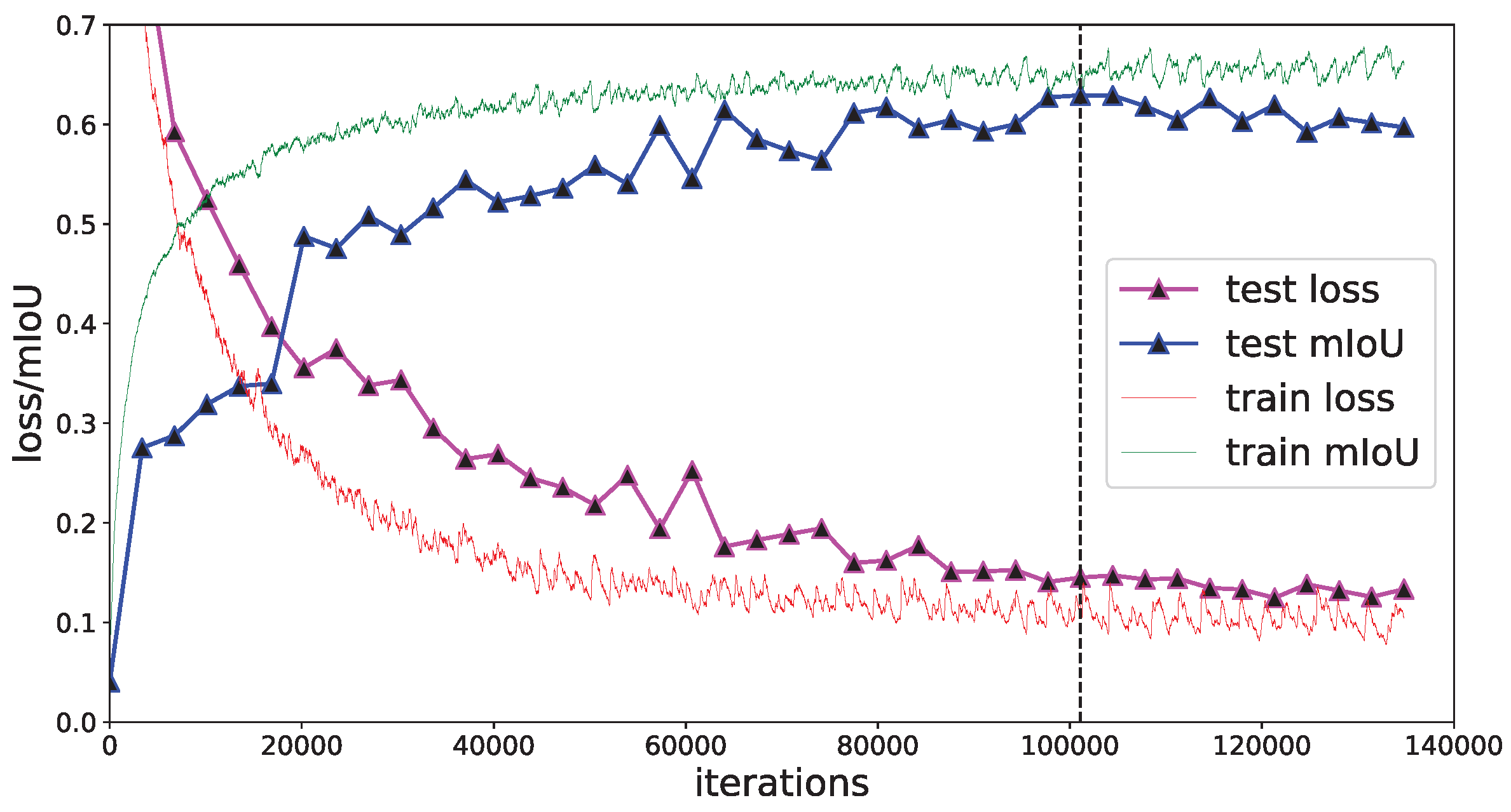
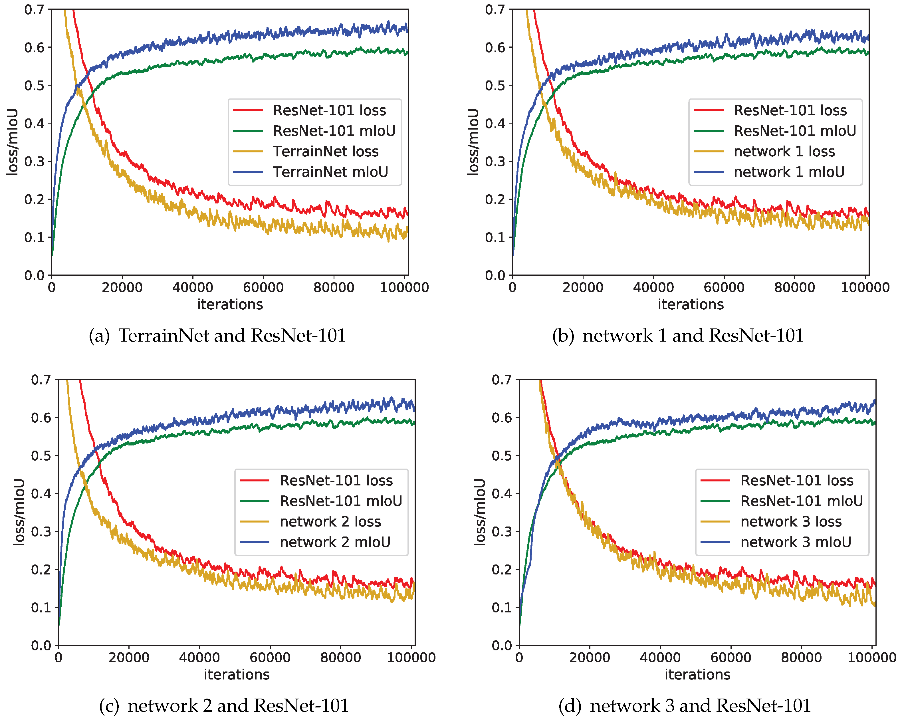
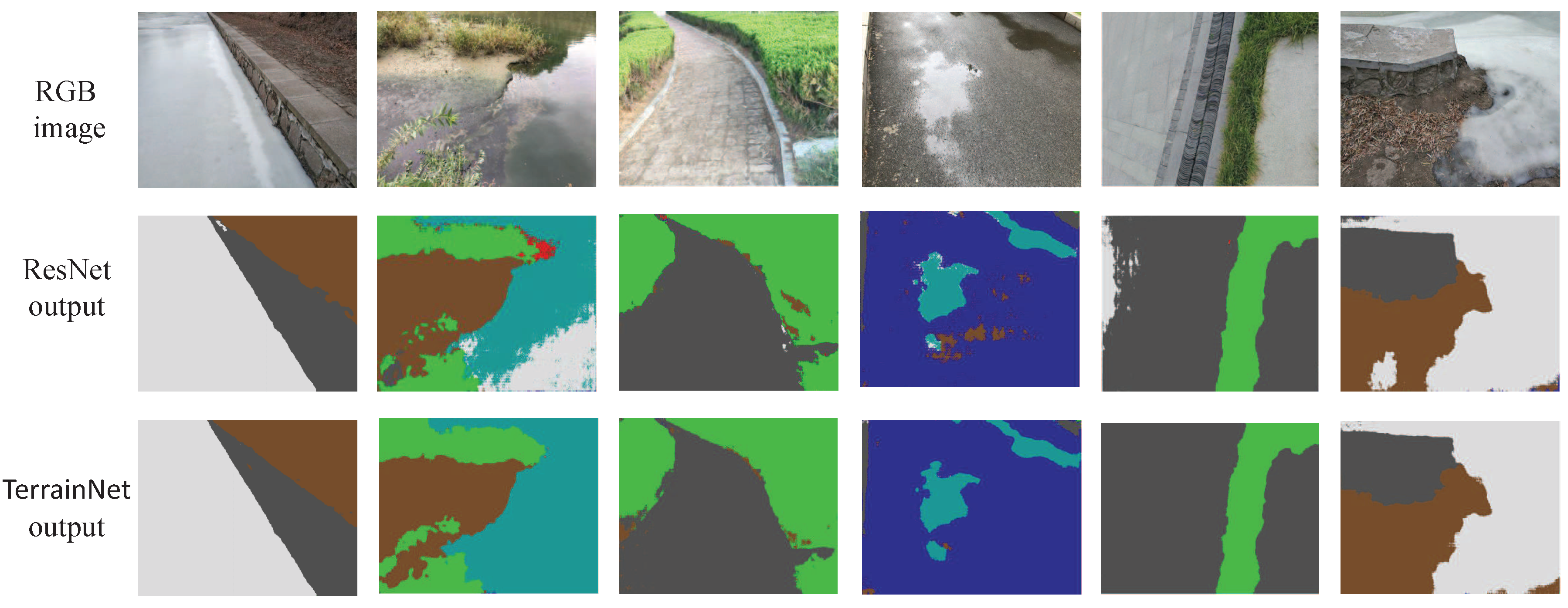
3.1. TerrainNet Experiment
3.2. Vision-Based Two-Stage Framework Experiment
4. Conclusions
Author Contributions
Funding
Conflicts of Interest
References
- Reggeti, J.C.A.; Armada, E.G. Parameter Identification and Modeling of Contact Properties for Robotic Applications. Ph.D. Thesis, Universidad Politécnica de Madrid, Madrid, Spain, 2017. [Google Scholar]
- Miller, B.D.; Cartes, D.; Clark, J.E. Leg stiffness adaptation for running on unknown terrains. In Proceedings of the 2013 IEEE/RSJ International Conference on Intelligent Robots and Systems, Tokyo, Japan, 3–7 November 2013; pp. 5108–5113. [Google Scholar]
- Lin, Y.C.; Ponton, B.; Righetti, L.; Berenson, D. Efficient humanoid contact planning using learned centroidal dynamics prediction. In Proceedings of the 2019 International Conference on Robotics and Automation (ICRA), Montreal, Canada, 20–24 May 2019; pp. 5280–5286. [Google Scholar]
- Giftsun, N.; Del Prete, A.; Lamiraux, F. Robustness to Inertial Parameter Errors for Legged Robots Balancing on Level Ground. In Proceedings of the 2017 International Conference on Informatics in Control, Automation and Robotics, Madrid, Spain, 27 July 2017. hal-01533136. [Google Scholar]
- Herzog, A.; Rotella, N.; Mason, S.; Grimminger, F.; Schaal, S.; Righetti, L. Momentum control with hierarchical inverse dynamics on a torque-controlled humanoid. Auton. Robot. 2016, 40, 473–491. [Google Scholar] [CrossRef]
- Konduri, S.; Orlando, E.; Torres, C.; Pagilla, P.R. Effect of wheel slip in the coordination of wheeled mobile robots. IFAC Proc. Vol. 2014, 47, 8097–8102. [Google Scholar] [CrossRef]
- Wang, C.; Meng, L.; She, S.; Mitchell, I.M.; Li, T.; Tung, F.; Wan, W.; Meng, M.Q.H.; de Silva, C.W. Autonomous mobile robot navigation in uneven and unstructured indoor environments. In Proceedings of the 2017 IEEE/RSJ International Conference on Intelligent Robots and Systems (IROS), Vancouver, BC, Canada, 24–28 September 2017; pp. 109–116. [Google Scholar]
- Qin, T.; Li, P.; Shen, S. Vins-mono: A robust and versatile monocular visual-inertial state estimator. IEEE Trans. Robot. 2018, 34, 1004–1020. [Google Scholar]
- Hogg, R.W.; Rankin, A.L.; Roumeliotis, S.I.; McHenry, M.C.; Helmick, D.M.; Bergh, C.F.; Matthies, L. Algorithms and sensors for small robot path following. In Proceedings of the 2002 IEEE International Conference on Robotics and Automation (Cat. No. 02CH37292), Washington, DC, USA, 11–15 May 2002; Volume 4, pp. 3850–3857. [Google Scholar]
- Mastalli, C.; Focchi, M.; Havoutis, I.; Radulescu, A.; Calinon, S.; Buchli, J.; Caldwell, D.G.; Semini, C. Trajectory and foothold optimization using low-dimensional models for rough terrain locomotion. In Proceedings of the 2017 IEEE International Conference on Robotics and Automation (ICRA), Singapore, 29 May–3 June 2017; pp. 1096–1103. [Google Scholar]
- Wang, K.; Ding, W.; Shen, S. Quadtree-accelerated real-time monocular dense mapping. In Proceedings of the 2018 IEEE/RSJ International Conference on Intelligent Robots and Systems (IROS), Madrid, Spain, 1–5 October 2018; pp. 1–9. [Google Scholar]
- Ding, L.; Gao, H.; Deng, Z.; Song, J.; Liu, Y.; Liu, G.; Iagnemma, K. Foot–terrain interaction mechanics for legged robots: Modeling and experimental validation. Int. J. Robot. Res. 2013, 32, 1585–1606. [Google Scholar] [CrossRef]
- Tsaprounis, C.; Aspragathos, N.A. A linear differential formulation of friction forces for adaptive estimator algorithms. Robotica 2001, 19, 407–421. [Google Scholar] [CrossRef]
- Fnadi, M.; Plumet, F.; Benamar, F. Nonlinear Tire Cornering Stiffness Observer for a Double Steering Off-Road Mobile Robot. In Proceedings of the 2019 International Conference on Robotics and Automation (ICRA), Montreal, QC, Canada, 20–24 May 2019; pp. 7529–7534. [Google Scholar]
- Fleming, R.W.; Wiebel, C.; Gegenfurtner, K. Perceptual qualities and material classes. J. Vis. 2013, 13, 9. [Google Scholar] [CrossRef] [PubMed]
- Tiest, W. Visual and haptic perception of roughness. Perception 2005, 34, 45–46. [Google Scholar]
- Hiramatsu, C.; Goda, N.; Komatsu, H. Transformation from image-based to perceptual representation of materials along the human ventral visual pathway. Neuroimage 2011, 57, 482–494. [Google Scholar] [CrossRef] [PubMed]
- Tang, J.; Ren, Y.; Liu, S. Real-time robot localization, vision, and speech recognition on Nvidia Jetson TX1. arXiv 2017, arXiv:1705.10945. [Google Scholar]
- Lee, K.; Lee, K.; Min, K.; Zhang, Y.; Shin, J.; Lee, H. Hierarchical novelty detection for visual object recognition. In Proceedings of the IEEE Conference on Computer Vision and Pattern Recognition, Salt Lake City, UT, USA, 18–22 June 2018; pp. 1034–1042. [Google Scholar]
- Ummenhofer, B.; Zhou, H.; Uhrig, J.; Mayer, N.; Ilg, E.; Dosovitskiy, A.; Brox, T. Demon: Depth and motion network for learning monocular stereo. In Proceedings of the IEEE Conference on Computer Vision and Pattern Recognition, Honolulu, HI, USA, 21–26 July 2017; pp. 5038–5047. [Google Scholar]
- Rosinol, A.; Sattler, T.; Pollefeys, M.; Carlone, L. Incremental Visual-Inertial 3D Mesh Generation with Structural Regularities. In Proceedings of the 2019 International Conference on Robotics and Automation (ICRA), Montreal, QC, Canada, 20–24 May 2019; pp. 8220–8226. [Google Scholar]
- Cordts, M.; Omran, M.; Ramos, S.; Rehfeld, T.; Enzweiler, M.; Benenson, R.; Franke, U.; Roth, S.; Schiele, B. The cityscapes dataset for semantic urban scene understanding. In Proceedings of the IEEE Conference on Computer Vision and Pattern Recognition, Las Vegas, NV, USA, 26 June–1 July 2016; pp. 3213–3223. [Google Scholar]
- Lin, T.Y.; Maire, M.; Belongie, S.; Hays, J.; Perona, P.; Ramanan, D.; Dollár, P.; Zitnick, C.L. Microsoft coco: Common objects in context. In Proceedings of the European Conference on Computer Vision, Zurich, Switzerland, 6–12 September 2014; pp. 740–755. [Google Scholar]
- Armeni, I.; Sax, S.; Zamir, A.R.; Savarese, S. Joint 2d-3d-semantic data for indoor scene understanding. arXiv 2017, arXiv:1702.01105. [Google Scholar]
- Pont-Tuset, J.; Perazzi, F.; Caelles, S.; Arbeláez, P.; Sorkine-Hornung, A.; Van Gool, L. The 2017 davis challenge on video object segmentation. arXiv 2017, arXiv:1704.00675. [Google Scholar]
- Caesar, H.; Uijlings, J.; Ferrari, V. Coco-stuff: Thing and stuff classes in context. In Proceedings of the IEEE Conference on Computer Vision and Pattern Recognition, Salt Lake City, UT, USA, 18–22 June 2018; pp. 1209–1218. [Google Scholar]
- Schilling, F.; Chen, X.; Folkesson, J.; Jensfelt, P. Geometric and visual terrain classification for autonomous mobile navigation. In Proceedings of the 2017 IEEE/RSJ International Conference on Intelligent Robots and Systems (IROS), Vancouver, BC, Canada, 24–28 September 2017; pp. 2678–2684. [Google Scholar]
- Garcia-Garcia, A.; Orts-Escolano, S.; Oprea, S.; Villena-Martinez, V.; Garcia-Rodriguez, J. A review on deep learning techniques applied to semantic segmentation. arXiv 2017, arXiv:1704.06857. [Google Scholar]
- Long, J.; Shelhamer, E.; Darrell, T. Fully convolutional networks for semantic segmentation. In Proceedings of the IEEE Conference on Computer Vision and Pattern Recognition, Boston, MA, USA, 7–12 June 2015; pp. 3431–3440. [Google Scholar]
- Badrinarayanan, V.; Kendall, A.; Cipolla, R. Segnet: A deep convolutional encoder-decoder architecture for image segmentation. IEEE Trans. Pattern Anal. Mach. Intell. 2017, 39, 2481–2495. [Google Scholar] [CrossRef] [PubMed]
- Chen, L.C.; Papandreou, G.; Schroff, F.; Adam, H. Rethinking atrous convolution for semantic image segmentation. arXiv 2017, arXiv:1706.05587. [Google Scholar]
- He, K.; Zhang, X.; Ren, S.; Sun, J. Deep residual learning for image recognition. In Proceedings of the IEEE Conference on Computer Vision and Pattern Recognition, Las Vegas, NV, USA, 27–30 June 2016; pp. 770–778. [Google Scholar]
- Adelson, E.H. On seeing stuff: The perception of materials by humans and machines. In Proceedings of the Human Vision and Electronic Imaging VI. International Society for Optics and Photonics, San Jose, CA, USA, 8 June 2001; Volume 4299, pp. 1–12. [Google Scholar]
- Komatsu, H.; Goda, N. Neural mechanisms of material perception: Quest on Shitsukan. Neuroscience 2018, 392, 329–347. [Google Scholar] [CrossRef] [PubMed]
- Bajracharya, M.; Ma, J.; Malchano, M.; Perkins, A.; Rizzi, A.A.; Matthies, L. High fidelity day/night stereo mapping with vegetation and negative obstacle detection for vision-in-the-loop walking. In Proceedings of the 2013 IEEE/RSJ International Conference on Intelligent Robots and Systems, Tokyo, Japan, 3–7 November 2013; pp. 3663–3670. [Google Scholar]
- Wooden, D.; Malchano, M.; Blankespoor, K.; Howardy, A.; Rizzi, A.A.; Raibert, M. Autonomous navigation for BigDog. In Proceedings of the 2010 IEEE International Conference on Robotics and Automation, Anchorage, AK, USA, 3–7 May 2010; pp. 4736–4741. [Google Scholar]
- Deng, F.; Zhu, X.; He, C. Vision-based real-time traversable region detection for mobile robot in the outdoors. Sensors 2017, 17, 2101. [Google Scholar] [CrossRef] [PubMed]
- Shinzato, P.Y.; Fernandes, L.C.; Osorio, F.S.; Wolf, D.F. Path recognition for outdoor navigation using artificial neural networks: Case study. In Proceedings of the 2010 IEEE International Conference on Industrial Technology, Vina del Mar, Chile, 14–17 March 2010; pp. 1457–1462. [Google Scholar]
- Russell, B.C.; Torralba, A.; Murphy, K.P.; Freeman, W.T. LabelMe: A database and web-based tool for image annotation. Int. J. Comput. Vis. 2008, 77, 157–173. [Google Scholar]
- Ng, A. Machine Learning Yearning. 2017. Available online: http://www.mlyearning.org/(96) (accessed on 9 June 2018).
- Kingma, D.P.; Ba, J. Adam: A method for stochastic optimization. arXiv 2014, arXiv:1412.6980. [Google Scholar]
- Kanopoulos, N.; Vasanthavada, N.; Baker, R.L. Design of an image edge detection filter using the Sobel operator. IEEE J. Solid-State Circuits 1988, 23, 358–367. [Google Scholar] [CrossRef]
- Silva, M.F.; Machado, J.T.; Lopes, A.M. Modelling and simulation of artificial locomotion systems. Robotica 2005, 23, 595–606. [Google Scholar] [CrossRef]
- Breiman, L.; Friedman, J.; Stone, C.J.; Olshen, R.A. Classification and Regression Trees; CRC Press: Boca Raton, FL, USA, 1984. [Google Scholar]


| Terrain in Different States | ||
|---|---|---|
| land 1 | 202.2 | 15.9 |
| land 2 | 169.1 | 14.6 |
| land 3 | 125.2 | 20.0 |
| land 4 | 88.1 | 8.6 |
| rock 1 | 228.6 | 10.5 |
| rock 2 | 123.7 | 22.8 |
| rock 3 | 154.3 | 21.9 |
| ice 1 | 190.4 | 12.7 |
| ice 2 | 161.2 | 22.8 |
| asphalt road 1 | 158.4 | 17.8 |
| asphalt road 2 | 113.3 | 5.5 |
| Terrain in Different States | ||
|---|---|---|
| land 1 | 15.7 | 5.6 |
| land 2 | 108.6 | 15.9 |
| land 3 | 40.3 | 8.9 |
| land 4 | 57.9 | 11.4 |
| rock 1 | 19.0 | 4.8 |
| rock 2 | 47.1 | 10.9 |
| rock 3 | 79.8 | 22.6 |
| ice 1 | 8.3 | 3.6 |
| ice 2 | 33.1 | 7.9 |
| asphalt road 1 | 61.8 | 9.3 |
| asphalt road 2 | 84.1 | 12.2 |
| Range of Value | 0– 64.2 | 64.2– 90.0 | 90.0– 112.8 | 112.8– 128.3 | 128.3– 150.8 | 150.8– 176.4 | 176.4– 192.3 | 192.3– 208.2 | 208.2– 224.5 | 224.5– 246.9 | 246.9– 255 |
| cluster number | 1 | 2 | 3 | 4 | 5 | 6 | 7 | 8 | 9 | 10 | 11 |
| Range of Value | 0–31.7 | 31.7–47.4 | 47.4–70.3 | 70.3–95.7 | 95.7–129.0 | 129.0–146.1 | 146.1–255 |
| cluster number | 1 | 2 | 3 | 4 | 5 | 6 | 7 |
| Level | 1 | 2 | 3 | 4 | 5 |
|---|---|---|---|---|---|
| friction coefficient | <0.1 | 0.1–0.25 | 0.25–0.5 | 0.5–0.7 | 0.7–0.8 |
| Level | 1 | 2 | 3 | 4 |
|---|---|---|---|---|
| stiffness (Nm) | 5.7 × 10 | 1.6 × 10–3.4 × 10 | 1.7 × 10 | 2.3 × 10–3.4 × 10 |
| Semantic ID | Cluster Number (Optical) | Cluster Number (Surface Structure) | Friction Level | Stiffness Level |
|---|---|---|---|---|
| 0 | — | — | 3 | 2 |
| 1 | 7,8,9,10,11 | 1 | 4 | 3 |
| 1 | 6,7,8,9 | 4,5,6,7 | 3 | 2 |
| 1 | 4,5,6 | 2,3 | 4 | 2 |
| 1 | 2,3 | 3,4 | 2 | 1 |
| 2 | 8,9,10,11 | 1,2 | 3 | 4 |
| 2 | 2,3,4,5 | 2,3 | 4 | 4 |
| 2 | 5,6,7,8 | 4,5,6 | 5 | 4 |
| 3 | 6,7,8,9 | 1 | 1 | 4 |
| 3 | 3,4,5,6,7,8 | 2,3 | 2 | 4 |
| 4 | — | — | 0 | 0 |
| 5 | 6,7,8,9,10 | 2,3,4 | 5 | 4 |
| 5 | 3,4,5 | 4,5 | 3 | 4 |
| 6 | — | — | 0 | 0 |
| Network Structure | mIoU (Train) | mIoU (Test) | Improvement (Test) |
|---|---|---|---|
| ResNet-101 (baseline) | 58.89% | 52.26% | — |
| network 1 | 63.31% | 59.08% | +6.28% |
| network 2 | 64.11% | 60.39% | +8.13% |
| network 3 | 63.72% | 59.27% | +7.01% |
| TerrainNet | 66.52% | 62.94% | +10.68% |
| Terrain | Grassland | Land | Rock | Ice | Water | Asphalt Road |
|---|---|---|---|---|---|---|
| 79.10% | 63.74% | 65.24% | 57.56% | 53.38% | 64.02% |
| Network | mIoU (Train) | mIoU (Test) |
|---|---|---|
| FCN | 52.31% | 49.64% |
| SegNet | 50.32% | 47.45% |
| DeepLabv3 | 63.84% | 60.24% |
| TerrainNet | 66.52% | 62.94% |
| Property | PA | mIoU |
|---|---|---|
| friction property | 75.85% | 60.18% |
| stiffness property | 76.63% | 61.21% |
© 2020 by the authors. Licensee MDPI, Basel, Switzerland. This article is an open access article distributed under the terms and conditions of the Creative Commons Attribution (CC BY) license (http://creativecommons.org/licenses/by/4.0/).
Share and Cite
Dong, Y.; Guo, W.; Zha, F.; Liu, Y.; Chen, C.; Sun, L. A Vision-Based Two-Stage Framework for Inferring Physical Properties of the Terrain. Appl. Sci. 2020, 10, 6473. https://doi.org/10.3390/app10186473
Dong Y, Guo W, Zha F, Liu Y, Chen C, Sun L. A Vision-Based Two-Stage Framework for Inferring Physical Properties of the Terrain. Applied Sciences. 2020; 10(18):6473. https://doi.org/10.3390/app10186473
Chicago/Turabian StyleDong, Yunlong, Wei Guo, Fusheng Zha, Yizhou Liu, Chen Chen, and Lining Sun. 2020. "A Vision-Based Two-Stage Framework for Inferring Physical Properties of the Terrain" Applied Sciences 10, no. 18: 6473. https://doi.org/10.3390/app10186473
APA StyleDong, Y., Guo, W., Zha, F., Liu, Y., Chen, C., & Sun, L. (2020). A Vision-Based Two-Stage Framework for Inferring Physical Properties of the Terrain. Applied Sciences, 10(18), 6473. https://doi.org/10.3390/app10186473