Electromagnetic Induction Imaging with Atomic Magnetometers: Progress and Perspectives

Abstract

Electromagnetic induction imaging (EMI) allows mapping of the conductivity of target objects and, when combined with appropriate algorithms, the generation of full 3D tomographic images. Despite its tremendous potential, and the wealth of possible applications, the use of EMI has essentially been limited to eddy current testing for monitoring of corrosion and welding in metallic structures. The present work reviews the factors hindering the progress of electromagnetic induction imaging and highlights how the use of atomic magnetometers overcame some of them, opening the path to real world applications of EMI. Perspectives for further developments are discussed.

1. Introduction

Electromagnetic induction imaging (EMI) allows mapping of the electromagnetic properties of an object. It is not limited to two-dimensional maps and, when combined with appropriate inversion algorithms, it can produce full three-dimensional images. Precisely to highlight such tomographic capabilities, it is often referred to as magnetic induction tomography (MIT) [1].

Potential applications of EMI cover a wide range of fields, from industrial monitoring to security screening and biomedical imaging. However, severe technical limitations, mostly due to the sensor, have so far limited the use of EMI to the detection of cracks and corrosion in metallic structures, a procedure usually termed eddy-current testing (ECT).

This article is aimed at reviewing the motivations which led to the development of EMI with atomic magnetometers, the key enabling role they played in overcoming important limitations of EMI, and the progress so far. Perspectives for future developments are discussed.

This work is organised as follows. In Section 2, the basic principles of the technique are reviewed. Section 3 discusses potential application areas for EMI and highlights the limitations of conventional inductive coils for these applications. Section 4 reviews the first demonstration of EMI with atomic magnetometers, and then covers in detail progress achieved in different application areas using the atomic sensors. Section 5 summarises the state-of-the-art of EMI with atomic magnetometers and identifies paths for future developments.

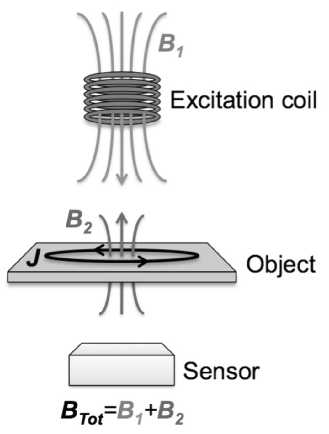
2. Principles of Electromagnetic Induction Imaging

Electromagnetic induction imaging relies on the active probing of the conductivity $\sigma$, permittivity $\epsilon$ and permeability $\mu$ of a target object by a weak oscillating magnetic field.

As sketched in Figure 1, in its simplest arrangement, an EMI device uses a primary magnetic field ($B_1$), generated by an induction coil and oscillating at a desired frequency, $\omega$. The primary field induces eddy currents (J) in the sample of interest. An important parameter for EMI applications is the skin depth $\delta$,

$$\delta =\sqrt{\frac{2}{\sigma \omega \mu }}\sqrt{\sqrt{1+{\left(\frac{\omega ϵ}{\sigma }\right)}^2}+\frac{\omega ϵ}{\sigma }},$$

(1)

which defines the depth below the surface of the conductor at which the current density has fallen to 1/e, and, as it will be discussed in the following, is a key parameter to characterise the EMI penetrating power.

The eddy currents induced in the material by the primary field produce in turn a secondary field ($B_2$), oscillating at $\omega$. The properties of the secondary field, in particular its amplitude and phase lag with respect with the primary field, depend on the specimen’s $\sigma$, $\epsilon$, and $\mu$. Therefore, by measuring $B_2$ at different positions, the dielectric characteristics of the sample can be mapped, and its image can be created. For simple planar geometries, a conductivity map can be constructed simply with a point-by-point derivation of the conductivity from individual measurements. For more complex 3D structures, the formation of a tomographic image involves the use of backprojection alghoritms [2] or the numerical solution of the inverse problem of electromagnetism [3].

In general, the response of the sample is a complicated function of the parameters of the geometrical arrangements. We refer here to a simple arrangement which leads to a transparent analytic expression for the sample response, useful to capture the underlying principles of EMI. We consider a uniform disc of material placed coaxially with, and midway between, an exciter coil and a sensor coil, with the separation of the coils assumed to be large compared with their diameters. Under the condition that the penetration depth of the exciter magnetic field in the sample is much larger than the sample thickness, it is possible to show that the the relative change $\Delta B/B$ in the receiver coil is given by [4,5]:

$$\frac{\Delta B}{B}=Q\omega {\mu }_0\left[\omega {ϵ}_0\left({ϵ}_r-1\right)-i\sigma \right]+R\left({\mu }_r-1\right),$$

(2)

where ${ϵ}_0$ is the vacuum permittivity, ${ϵ}_r$ the relative permittivity of the sample material, and ${\mu }_r$ its relative magnetic permeability. The quantities Q and R are geometrical factors.

Equation (2) highlights the different contributions of the sample response to the variation in magnetic field recorded by the receiver coil. We note that the three different components, determined by the material permittivity, conductivity and pearmeability, can be separated by using their different dependence on the driving frequency and different phase relation. In most practical applications, the response is usually dominated by the conductivity contribution.

3. Application Areas and Limitations of Inductive Coils

3.1. Security

Luggage, cargo and vehicle screening play an important role in ensuring transport security. X-ray based scanners are a very effective tool for this application, because of their ability to image through barriers. However, the use of ionising radiation requires adopting precautions for the operators as well as for the members of public. This constitutes a potentially serious drawback of X-ray scanners for security. In this context, electromagnetic induction imaging was considered due to its harmless nature. The demonstration [6,7,8] of the ability of electromagnetic imaging to penetrate through metallic barriers validated its potential use for security applications. However, increased penetration requires lowering of the operating frequency, typically below the 1 MHz level, as from the expression (1) for the skin depth. Conventional inductive sensors are severely challenged at such low frequencies, with a very significant loss of sensitivity.

3.2. Surveillance

Magnetic sensors are routinely used for surveillance, e.g., for underwater detection. However, this relies on the spontaneous magnetisation of the object of interest, which can be reduced by an appropriate choice of the materials used in the object construction and the adoption of degaussing processes. Furthermore, passive detection of spontaneous magnetisation is affected by ambient noise. Detection systems based on electromagnetic induction are superior in this respect, as they rely on the target’s conductivity, rather than its magnetisation, which is less suitable for the implementation of countermeasures. Furthermore, the active nature of electromagnetic induction detection system allows for the use of lock-in techniques, which significantly reduce the detrimental effect of ambient noise. However, inductive coil based sensors are not suitable as the required penetration of the magnetic field through several hundred of meters of water requires, as from (1), the operation of the system at low frequency, in a range (1–100 kHz) where the performance of inductive coils is severely degraded.

3.3. Biomedical Imaging

Several medical conditions are associated with a variation of the conductivity of the tissues affected by the specific disorder. Such a variation may be the cause or the consequence of such illness. In any case, it represents a marker of many conditions. These include: head injuries, atrial fibrillation and cancer. EMI is the natural tool to detect and characterise these conductivity anomalies. The potential of EMI for biodemedical imaging was recognised long time ago [9]. Advantages of EMI for specific conditions are reviewed here.

3.3.1. Head Injuries

Head injuries, and in particular Intra-Cerebral Haemorrhage (ICH) and Cerebral Oedema (COE), correspond to excess of fluids in the intracranial region and require a rapid assessment to increase the chances of survival and to contain long-term consequences, potentially life-changing. The excess of fluid produces an anomaly in the conductivity of the brain tissue, which can in principle be detected via electromagnetic induction imaging techniques [4,10]. However, this is very challenging, as in the case of ICH or COE, the encephalic regions occupied by fluids are only fractionally more conductive than the surrounding healthy tissue. On average, cerebrospinal fluid (CSF) and blood are 20 and 10 times, respectively, more conductive than the normal brain tissue (white matter) [11]. However, an EMI system with suitable performance would be able to identify the areas occupied by an excess of fluid, even with different levels of perfusion and hence different average conductivity [12]. Furthermore, if the EMI system has sufficient conductivity resolution, it will have the potential to distinguish the nature of the fluids involved, namely blood (ICH) or plasma/CSF (COE).

EMI systems have inherently low-resolution, and in this respect they do not appear capable of competing with any MRI or CT scanners currently available. However, in case of head injuries, high resolution is not a requirement for the initial assessment of the injury as well as for monitoring the evolution of mild head traumas in the longer term. Additionally, EMI systems would have the major advantage of being easily deployable on the field. Head injuries need a rapid assessment, as the fluid build up leads to an increased intracranial pressure which may quickly lead to brain injuries. MRI and CT scan systems are bulky and expensive, so are not easily deployable. In contrast, low-cost and easy to operate EMI systems could be promptly available in all the settings (e.g., sport events, battlefield, ski resorts etc.) where head injuries occur more frequently. As the magnetic fields required by EMI for biomagnetism are very small and the lasers are very low power (typically ∼1 mW), the device is suitable for battery operation. Furthermore, EMI devices are low weight and very compact, thus easily transportable. EMI devices are also potentially suitable for prolonged or continuous monitoring, unlike MRI or CT scanners, which pose potential risks for the patient and unacceptable financial strain. In this respect, we notice here that the rf field used in EMI is very weak (of the order of 1 nT). For the frequency of interest—in the MHz range—there is no evidence that this may be harmful. However, systematic studies have yet to be performed.

3.3.2. Cancer

Cancerous tissues are characterized by a significant variation in conductivity with respect to the surrounding healthy tissues. Specifically, in presence of a cancer, the conductivity of liver and lung tissues increases by more than 30%, and by more than 500% in the case of mammary tissue [13]. The discussion of the physiological processes leading to such a difference is well beyond the scope of this work. One may argue that—as the electrical conductivity in live tissues is largely determined by ion transport [14]—the contribution to the generation of the EMI signal from the structures involved in ion exchange may be dominant. However, other possible contributions cannot be ruled out.

The anomalous conductivity of cancerous tissue makes it detectable by electromagnetically induction imaging. However, cancer is routinely detected and precisely characterized by CT scans, so one may wonder whether low-resolution EMI may add anything at all to the available toolkit available for cancer diagnostics.

In the context of lung cancer, it was argued [15] that detection of early stage cancer could be the key to increase the 5-year survival rate. EMI may play a role in this direction and its low cost harmless nature makes it an ideal diagnostic tool for very widespread use.

3.3.3. Atrial Fibrillation

Cardiac arrhythmias are heart conditions characterized by irregular, slow, or accelerated, beating of the heart. Their causes are related to anomalies in the conduction of the electrical pulses that control the heart’s activity [16]. Among the most diffused sustained arrhythmias is atrial fibrillation (AF), which affects a substantial fraction of population over 70. It manifests as a turbulent cardiac activity and represents one of the most important causes of morbidity and mortality in rich countries [17]. Nevertheless, its clinical treatment, either via drug therapy [18] or surgical procedure, is sub-optimal [19].

Little is known about the fundamental causes and mechanisms of AF. Recently, the first indications of localized stable sources were found in patients referred for AF [20]. It was then argued that fibrillation is caused by permanent modification of the heart’s local conductivity, which produces deterministic sources known as rotors, and by the stochastic interaction with the local anatomy, which creates randomly distributed re-entry paths (wavelets). However, the topic is still widely debated.

Progress in understanding the mechanisms underlying atrial fibrillation, and improvements in the clinical practice, require new diagnostic tools. In fact, magnetocardiography (MCG) and electrocardiography (ECG) do not provide any direct information about the causes of the irregular beat and, more importantly, the structures producing it.

In 2016 magnetic induction tomography was proposed as novel approach to the diagnosis of fibrillations [21,22]. In fact, EMI has the potential to generate a non-invasive, space-resolved map of the heart’s conductivity, thus addressing directly the presence of permanent conduction anomalies and their relationship with the on-set and the dynamics of fibrillation. However, the sensitivity required for EMI of the hearth surpasses by far the performances of conventional inductive sensors.

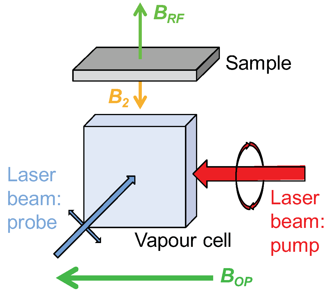
4. Electromagnetic Induction Imaging with Atomic Magnetometers

4.1. Motivations

Conventional EMI/MIT systems rely on a set of coils to detect the secondary field’s contributions. In this way, the performance and the imaging capability can be severely limited by the performance of the coils. Consequently, coil-based EMI has limited sensitivity below 50 MHz. This prevented the successful implementation of EMI for biological tissues, which produce very small secondary fields due to their very low conductivity ($\sigma \simeq 1$ S/m) and also in security and surveillance, where it is often necessary to operate the EMI systems at a frequency well below 1 MHz to achieve penetration through metallic shields or significant depths of water.

To overcome these limitations in sensitivity, the use of atomic magnetometers [23] for the detection of the secondary field was proposed and demonstrated in 2013 [24]. AMs have extreme sensitivity (≤${10}^{-15}$ T$/\sqrt{\mathrm{Hz}}$), comparable to the performances of super-conductive quantum interference devices (SQUIDs) [23]. In contrast to SQUIDs, AMs are capable of room temperature and unshielded operation. Of particular importance for EMI applications, AMs retain their sensitivity also at very low frequencies, and notably below 50 MHz their sensitivity can be up to ${10}^7$ times larger than that of a standard pick-up coil of the same size [25]. This was the main motivation behind the work which ultimately led to the implementation of EMI with atomic magnetometers.

4.2. First Proof-Of-Concept of EMI with Atomic Magnetometers

The demonstration of magnetic induction measurements with an atomic magnetometer [24] was followed by the first proof-of-concept demonstration of EMI with the same atomic sensor [26]. In those works, a self-oscillating atomic magnetometer [27,28] was used. The core of the magnetometer was a vapor cell, filled with the naturally occurring mixture of rubidium, heated to 70 ${}^{°}$C to increase the vapor density, and buffer gas. Images of a square, triangle and disk of 2 mm aluminium were successfully generated by position resolved measurement, obtained by moving the object with respect to the sensor. The original images are reproduced in Figure 2. These were the very first images produced via electromagnetic induction imaging using an atomic magnetometer as the sensor.

The proof-of-concept demonstration reported in [26] opened up new prospects for EMI as atomic magnetometers have the potential to reach the sensitivity at low frequency required for essentially all EMI applications. This required further development to fully exploit the exquisite sensitivity of atomic magnetometers, as described below.

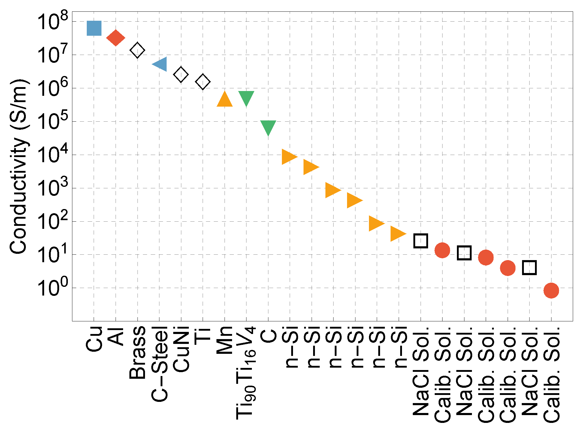
4.3. Development of EMI with AMs and the Quest for Ultimate Sensitivity

Progress of EMI with atomic magnetometer beyond the proof-of-concept first involved the identification of the AM configurations best suited for the task. While the first proof of concept used a self-oscillating AM [26], further parallel development by the UCL [29] and the Mainz groups [30] was based on the so-called radio-frequency atomic magnetometer [31], a configuration specially devised to measure rf fields, which was found more suitable for the implementation of EMI. In this configuration, shown in Figure 3, atoms contained in a glass cell are polarized via optical pumping with a circularly polarised laser beam propagating collinearly to an applied bias field. Spin precession is driven by an applied rf field, and probed by a linearly polarized laser field propagating perpendicularly to the bias field. The probe beam polarization direction oscillates at the frequency of the rf driving field, with the amplitude and phase of the oscillating polarization measured by a lock-in amplifier.

The RF-AM does not require any modification to operate in electromagnetic imaging modality. The sample of interest is introduced in the vicinity of the atomic magnetometer. The coil driving the atomic spin precession in the magnetometer plays now the additional role of inducing eddy currents in the sample, with the amplitude and phase of the resulting secondary field read by the atomic magnetometer.

The demonstration of EMI with RF-AMs opened up a series of investigations targeting specific applications, leading also to further technical developments.

In the period 2015–2017, the potential of the EMI-AM system for through-barrier imaging was investigated [32,33]. An important requirement for security is the ability to penetrate conductive barriers which may also be ferromagnetic. In [33], detrimental effects due to the ferromagnetic barriers, including unpredictable magnetic signatures from ferromagnetic screens and variations in the magnetic background, were automatically compensated by active compensation coils controlled by servo loops. Imaging of multiple conductive targets concealed by a 2.5 mm ferromagnetic steel shield and/or a 2.0 mm aluminium shield, in a single scan was reported, thus validating the technique for security applications.

In 2018, a proof-of-concept of active underwater detection and tracking was reported with an array of four RF-AMs operating in EMI modality [34]. This demonstrated a detection principle different from the conventional measurement of residual spontaneous magnetisation of the object of interest, and finds direct application in underwater surveillance. In this context, it has the significant advantage over conventional detection systems that it relies on the object conductivity only, and thus degaussing procedures are not an effective countermeasure. Of course, one may also argue that being an active system has the disadvantage of potentially revealing the presence of the observer, although this is mitigated by the weakness and narrow band of the rf field used as exciter.

The application area which led to the most significant progress in EMI-AM technology is the biomedical one, with mapping of the heart conductivity, identified in [21] as a new approach to the diagnostics of atrial fibrillation, a specific goal. Mapping the conductivity of biological tissue requires exteme sensitivity, so to be able to image structure with volumes of a few ml and conductivity of the order of 1–10 S/m. This stimulated a continuous development of the performances of EMI-AM systems [35,36]. This rapidly led to the demonstration [37] of imaging of a few mL of calibrated saline solution with conductivity below 1 S/m, as required for biomedical imaging. Figure 4 illustrates this development from the early demonstrations to the state-of-the-art sensititivity measurements of [37] by reporting the milestones in the quest for extreme sensitivity to small volumes of low-conductive materials.

Among the various technical developments, two certainly played an essential role in reaching extreme sensitivity: the use of near-resonant imaging [35], and the introduction of the dual-coil configuration for the rf-field [36,37,38]. Near-resonant imaging consists in choosing the frequency of the rf field slightly different from exact atomic resonance. This may seem counterintuitive, as maximum sensitivity requires exact resonance. However, it was found that by slightly detuning the rf field an optimum compromise can be reached between absolute sensitivity of the magnetometer and robustness against ambient magnetic noise, which would otherwise degrade the image. This allows for the operation of the EMI-AM system with high sensitivity and stability over the duration of the measurement. The second key development, the dual-coil configuration, results from the observation that a larger primary field produces a corresponding increase of the amplitude secondary field produced by the object of interest, thus leading to an improvement in sensitivity. However, in a standard single coil configuration, the primary field also drives the atomic spin precession in the magnetometer. Thus an excessive increase results in the saturation of the atomic resonance, and a resulting decrease in sensitivity. A solution to this issue, already put forward in the context of MIT with inductive coils [1] and also implemented in the context of nuclear quadrupole resonance spectroscopy with RF-AMs [39], is the use of a dual-coil configuration, so to have a large field on the target object and a significantly reduced field driving the atomic spins.

4.4. Alghorithms for Image Reconstruction: The Machine Learning Approach

An important aspect of electromagnetic induction imaging is the ability of reconstructing an image given a finite set of measurements of secondary magnetic field amplitude and phase at different locations. This is a key enabling factor of the tomographic capability of EMI. The standard approach relies on the numerical solution of the inverse problem of electromagnetism, a challenging task given that the problem is ill-posed. This is still an active area of research, and a thorough discussion goes beyond the present work, whose focus is the progress determined by the use of atomic magnetometers. However, it is worth mentioning that an alternative approach, based on machine learning, was demonstrated in the context of EMI-AM precisely to avoid the complications related to the inverse problem approach. While machine learning is routinely used with standard ray-optics images, it is a priori not obvious that it could be applied to EMI given the diffusive non-ray-optics nature of the images. In this context, a proof-of-concept validation of machine learning for EMI-AM was provided in 2018 [40] for the mapping of bidimensional objects. Localization and classification of objects of different shape and material was demonstrated. The validation of machine learning based alghoritms for EMI is of great interest, as it offers an alternative to the often cumbersome solution of the inverse problem of electromagnetism. Whether this approach can be extended to complex and cluttered scenes, and to 3D systems is still an open question, and forms the object of ongoing research.

5. Discussion and Conclusions

Electromagnetic induction imaging has a long history, and many key use cases have been identified thoughout the years. However, EMI failed to fulfill its potential, as many factors limited its performances. An important factor was the loss of sensitivity of inductive sensors at low frequency. The demonstration of electromagnetic induction imaging with atomic magnetometers in 2014 showed how it was possible to overcome this, and opened up the path to a tremendous development, culminated with the demonstration in 2020 of imaging of a few ml of saline solutions with conductivity below 1 S/m, thus bringing EMI-AM in the domain of biomedical imaging. High sensitivity at low frequency also led to the demonstration of through-barrier imaging, of relevance to security applications. This development saw the involvement of many groups worlwide. Since the first demonstration at UCL [26], EMI-AM research was also conducted at the University of Mainz [30], the National Physical Laboratory [38,41,42,43,44,45] and the University of Copenhagen [36]. However, despite the tremendous progress in the sensitivity of the sensor, other limiting factors remain, and work is ongoing in different directions.

An important area where development is needed is image reconstruction. The standard approach relies on the solution of the inverse problem of electromagnetism, with a tomographic image constructed from measurmeents of the secondary field at a finite set of points. However, the problem is ill posed, the inversion is computationally challenging and a set of assumptions about the object at hand are required to make the procedure viable. Research on the inverse solution of the problem of electromagnetism is ongoing, and continuous progress is reported. An alternative approach is based on machine learning alghoritms. Widely used for ray-optics, the procedure was recently validated for the diffusive imaging of MIT, and investigations are in progress to evaluate its potential for complex and cluttered scenes.

Another important limitation of EMI is the low spatial resolution. Although EMI will never be able to compete with imaging systems based on ray-like propagation such as X rays, developments can be envisaged to improve the resolution of EMI-AM systems. For objects relatively far (cm or more) from the sensor, an important limiting factor is the spreading of the primary field, which induces eddy currents in the entire object. Selective excitation of eddy currents in different portions of the object would allow for better resolution. Improvements in this direction can be achieved by primary field shaping, moving away from the standard single coil design and adopting more complex schemes based on the solution of optimisation problems. Of interest to nanotechnolgy is also the case where the sample is in close proximity of the sensor, with the aim to produce high-resolution conductivity maps. In this case, an important limiting factor is the size of the sensor. Instead of using relatively (few mm) large ensembles of atoms in a vapour cell, progress can be made by adopting ultra-cold atom systems, with atomic clouds of few tens of micron size in close proximity to the object surface. A first step in this direction was recently achieved with the demonstration of a cold atom RF-AM [46], which can be used for EMI. It is worth mentioning that for this specific application, where the minute size of the sensor plays a central role, a valid alternative may also be constituted by NV diamond based EMI systems, as recently demonstrated by the Mainz group [47].

The entire development to date of EMI-AM systems, and resulting increase in sensitivity, has been based on AMs operating at best at the standard quantum limit. This limitation can be overcome, with a further increase in sensitivity, by using squeezed light or squeezed atomic spins [48]. Radio-frequency field detection below the standard quantum limit [49] may thus be the key to increase even further the ability of imaging low-conductivity samples. Of particular interest would be the increase of the sensitivity per atom, so to be able to maintain extreme sensitivity with smaller atomic samples. This would allow the improvement of the spatial resolution of the EMI technique at no cost in terms of sensitivity.

In conclusion, with the demonstration of EMI with atomic magnetometers, EMI technology has entered a new phase of development with real-world application now in sight.

References

1. Griffiths, H. Magnetic induction tomography. Meas. Sci. Technol. 2001, 12, 1126. [Google Scholar] [CrossRef]
2. Korjenevsky, A.; Cherepenin, V.; Sapetsky, S. Magnetic induction tomography: Experimental realization. Physiol. Meas. 2000, 21, 89–94. [Google Scholar] [CrossRef] [PubMed]
3. Merwa, R.; Hollaus, K.; Brandstaetter, B.; Scharfetter, H. Numerical solution of the general 3D eddy current problem for magnetic induction tomography (spectroscopy). Physiol. Meas. 2003, 24, 545–554. [Google Scholar] [CrossRef] [PubMed]
4. Scharfetter, H.; Casañas, R.C.; Rosell, J. Biological Tissue Characterization by Magnetic Induction Spectroscopy (MIS): Requirements and Limitations. IEEE Trans. Biomed. Eng. 2003, 50, 870–880. [Google Scholar] [CrossRef]
5. Griffiths, H.; Gough, W.; Watson, S.; Williams, R.J. Residual capacitive coupling and the measurement of permittivity in magnetic induction tomography. Physiol. Meas. 2007, 28, S301–S311. [Google Scholar] [CrossRef]
6. Darrer, B.J.; Watson, J.C.; Bartlett, P.; Renzoni, F. Magnetic Imaging: A New Tool for UK National Nuclear Security. Sci. Rep. 2015, 5, 7944. [Google Scholar] [CrossRef] [Green Version]
7. Darrer, B.J.; Watson, J.C.; Bartlett, P.A.; Renzoni, F. Electromagnetic imaging through thick metallic enclosures. AIP Adv. 2015, 5, 087143. [Google Scholar] [CrossRef] [Green Version]
8. Guilizzoni, R.; Watson, J.C.; Bartlett, P.; Renzoni, F. Penetrating power of resonant electromagnetic induction imaging. AIP Adv. 2016, 6, 095017. [Google Scholar] [CrossRef] [Green Version]
9. Alzeibak, S.; Saunders, N.H. A feasibility study of in vivo electromagnetic imaging. Phys. Med. Biol. 1993, 38, 151–160. [Google Scholar] [CrossRef]
10. Merwa, R.; Hollaus, K.; Biró, O.; Scharfetter, H. Detection of brain oedema using magnetic induction tomography: A feasibility study of the likely sensitivity and detectability. Phys. Meas. 2004, 25, 347–354. [Google Scholar] [CrossRef]
11. Pan, W.; Yan, Q.; Qin, M.; Jin, G.; Sun, J.; Ning, X.; Wei, Z.; Bin, P.; Gen, L. Detection of Cerebral Hemorrhage in Rabbits by Time-Difference Magnetic Inductive Phase Shift Spectroscopy. PLoS ONE 2015, 10, e0128127. [Google Scholar] [CrossRef] [PubMed]
12. Zolgharni, M.; Griffiths, H.; Ledger, P.D. Frequency-difference MIT imaging of cerebral haemorrhage with a hemispherical coil array: Numerical modelling. Physiol. Meas. 2010, 31, S111–S125. [Google Scholar] [CrossRef] [PubMed]
13. Joines, W.T.; Zhang, Y.; Li, C.; Jirtle, R.L. The measured electrical properties of normal and malignant human tissues from 50 to 900 MHz. Med. Phys. 1994, 21, 547–550. [Google Scholar] [CrossRef] [PubMed]
14. Gabriel, S.; Lau, R.W.; Gabriel, C. The dielectric properties of biological tissues: III. parametric models for the dielectric spectrum of tissues. Phys. Med. Biol. 1996, 41, 2271–2293. [Google Scholar] [CrossRef] [Green Version]
15. Wang, L.; Al-Jumaily, A.M. Imaging of Lung Structure Using Holographic Electromagnetic Induction. IEEE Access 2017, 5, 20313–20318. [Google Scholar] [CrossRef]
16. Longo, D.; Fauci, A.; Kasper, D.; Hauser, S.; Jameson, J.; Loscalzo, J. Harrison’s Principles of Internal Medicine, 18th ed.; McGraw Hill Professional: New York, NY, USA, 2012; Volume 2. [Google Scholar]
17. Vaquero, M.; Calvo, D.; Jalife, J. Cardiac fibrillation: From ion channels to rotors in the human heart. Heart Rhythm 2008, 5, 872–879. [Google Scholar] [CrossRef] [Green Version]
18. Christ, T.; Rozmaritsa, N.; Engel, A.; Berk, E.; Knaut, M.; Metzner, K.; Canteras, M.; Ravens, U.; Kaumannb, A. Arrhythmias, elicited by catecholamines and serotonin, vanish in human chronic atrial fibrillation. Proc. Natl. Acad. Sci. USA 2014, 111, 11193–11198. [Google Scholar] [CrossRef] [Green Version]
19. Narayan, S.M.; Patel, J.; Mulpuru, S.; Krummen, D.E. Focal impulse and rotor modulation ablation of sustaining rotors abruptly terminates persistent atrial fibrillation to sinus rhythm with elimination on follow-up: A video case study. Heart Rhythm 2012, 9, 1436–1439. [Google Scholar] [CrossRef] [Green Version]
20. Narayan, S.M.; Krummen, D.E.; Rappel, W.-J. Clinical Mapping Approach To Diagnose Electrical Rotors and Focal Impulse Sources for Human Atrial Fibrillation. J. Cardiovasc. Electrophysiol. 2012, 23, 447–454. [Google Scholar] [CrossRef] [Green Version]
21. Marmugi, L.; Renzoni, F. Optical Magnetic Induction Tomography of the Heart. Sci. Rep. 2016, 6, 23962. [Google Scholar] [CrossRef] [Green Version]
22. Deans, C.; Marmugi, L.; Hussain, S.; Renzoni, F. Optical atomic magnetometry for magnetic induction tomography of the heart. Proc. SPIE 2016, 9900, 99000F. [Google Scholar]
23. Budker, D.; Romalis, M. Optical magnetometry. Nat. Phys. 2007, 3, 227–234. [Google Scholar] [CrossRef] [Green Version]
24. Wickenbrock, A.; Tricot, F.; Renzoni, F. Magnetic induction measurements using an all-optical 87Rb atomic magnetometer. Appl. Phys. Lett. 2013, 103, 243503. [Google Scholar] [CrossRef] [Green Version]
25. Savukov, I.M.; Seltzer, S.J.; Romalis, M.V. Detection of NMR Signals With a Radio-Frequency Atomic Magnetometer. J. Magn. Reson. 2007, 185, 214–220. [Google Scholar] [CrossRef] [Green Version]
26. Wickenbrock, A.; Jurgilas, S.; Dow, A.; Marmugi, L.; Renzoni, F. Magnetic induction tomography using an all-optical 87Rb atomic magnetometer. Opt. Lett. 2014, 39, 6367. [Google Scholar] [CrossRef] [Green Version]
27. Schwindt, P.D.D.; Hollberg, L.; Kitching, J. Self-oscillating rubidium magnetometer using nonlinear magneto-optical rotation. Rev. Sci. Instrum. 2005, 76, 126103. [Google Scholar] [CrossRef] [Green Version]
28. Belfi, J.; Bevilacqua, G.; Biancalana, V.; Cartaleva, S.; Dancheva, Y.; Khanbekyan, K.; Moi, L. Dual channel self-oscillating optical magnetometer. J. Opt. Soc. Am. B 2009, 26, 910–916. [Google Scholar] [CrossRef]
29. Deans, C.; Marmugi, L.; Hussain, S.; Renzoni, F. Electromagnetic Induction Imaging with a Radio-Frequency Atomic Magnetometer. Appl. Phys. Lett. 2016, 108, 103503. [Google Scholar] [CrossRef]
30. Wickenbrock, A.; Leefer, N.; Blanchard, J.W.; Budker, D. Eddy current imaging with an atomic radio-frequency magnetometer. Appl. Phys. Lett. 2016, 108, 183507. [Google Scholar] [CrossRef] [Green Version]
31. Savukov, I.M.; Seltzer, S.J.; Romalis, M.V.; Sauer, K.L. Tunable atomic magnetometer for detection of radio-frequency magnetic fields. Phys. Rev. Lett. 2005, 95, 063004. [Google Scholar] [CrossRef] [Green Version]
32. Marmugi, L.; Hussain, S.; Deans, C.; Renzoni, F. Magnetic induction imaging with optical atomic magnetometers: Towards applications to screening and surveillance. Proc. SPIE 2015, 9652, 965209. [Google Scholar]
33. Deans, C.; Marmugi, L.; Renzoni, F. Through-barrier electromagnetic imaging with an atomic magnetometer. Opt. Express 2017, 25, 17911. [Google Scholar] [CrossRef] [PubMed]
34. Deans, C.; Marmugi, L.; Renzoni, F. Active Underwater Detection with an Array of Atomic Magnetometers. Appl. Opt. 2018, 57, 2346. [Google Scholar] [CrossRef]
35. Marmugi, L.; Deans, C.; Renzoni, F. Electromagnetic induction imaging with atomic magnetometers: Unlocking the low-conductivity regime. Appl. Phys. Lett. 2019, 115, 083503. [Google Scholar] [CrossRef]
36. Jensen, K.; Zugenmaier, M.; Arnbak, J.; Stærkind, H.; Balabas, M.V.; Polzik, E.S. Detection of low-conductivity objects using eddy current measurements with an optical magnetometer. Phys. Rev. Res. 2019, 1, 033087. [Google Scholar] [CrossRef] [Green Version]
37. Deans, C.; Marmugi, L.; Renzoni, F. Sub-Sm−1 electromagnetic induction imaging with an unshielded atomic magnetometer. Appl. Phys. Lett. 2020, 116, 133501. [Google Scholar] [CrossRef]
38. Bevington, P.; Gartman, R.; Chalupczak, W. Enhanced material defect imaging with a radio-frequency atomic magnetometer. J. Appl. Phys. 2019, 125, 094503. [Google Scholar] [CrossRef] [Green Version]
39. Lee, S.-K.; Sauer, K.L.; Seltzer, S.J.; Alem, O.; Romalis, M.V. Subfemtotesla radio-frequency atomic magnetometer for detection of nuclear quadrupole resonance. Appl. Phys. Lett. 2006, 89, 214106. [Google Scholar] [CrossRef] [Green Version]
40. Deans, C.; Griffin, L.D.; Marmugi, L.; Renzoni, F. Machine learning based localization and classification with atomic magnetometers. Phys. Rev. Lett. 2018, 120, 033204. [Google Scholar] [CrossRef]
41. Bevington, P.; Gartman, R.; Chalupczak, W.; Deans, C.; Marmugi, L.; Renzoni, F. Non-Destructive Structural Imaging of Steelwork with Atomic Magnetometers. Appl. Phys. Lett. 2018, 113, 063503. [Google Scholar] [CrossRef]
42. Bevington, P.; Gartman, R.; Chalupczak, W. Imaging of material defects with a radio-frequency atomic magnetometer. Rev. Sc. Instr. 2019, 90, 013103. [Google Scholar] [CrossRef] [PubMed]
43. Bevington, P.; Gartman, R.; Chalupczak, W. Alkali-metal spin maser for non-destructive tests. Appl. Phys. Lett. 2019, 115, 173502. [Google Scholar] [CrossRef]
44. Bevington, P.; Gartman, R.; Chalupczak, W. Magnetic induction tomography of structural defects with alkali–metal spin maser. Appl. Opt. 2020, 59, 2276–2282. [Google Scholar] [CrossRef] [PubMed]
45. Bevington, P.; Gartman, R.; Botelho, D.J.; Crawford, R.; Packer, M.; Fromhold, T.M.; Chalupczak, W. Object surveillance with radio-frequency atomic magnetometers. Rev. Sci. Instrum. 2020, 91, 055002. [Google Scholar] [CrossRef] [PubMed]
46. Cohen, Y.; Jadeja, K.; Sula, S.; Venturelli, M.; Deans, C.; Marmugi, L.; Renzoni, F. A cold atom radio-frequency magnetometer. Appl. Phys. Lett. 2019, 114, 073505. [Google Scholar] [CrossRef] [Green Version]
47. Chatzidrosos, G.; Wickenbrock, A.; Bougas, L.; Zheng, H.; Tretiak, O.; Yang, Y.; Budker, D. Eddy-current imaging with nitrogen-vacancy centers in diamond. Phys. Rev. Appl. 2019, 11, 014060. [Google Scholar] [CrossRef] [Green Version]
48. Giovannetti, V.; Lloyd, S.; Maccone, L. Quantum-Enhanced Measurements: Beating the Standard Quantum Limit. Science 2004, 306, 1330. [Google Scholar] [CrossRef] [Green Version]
49. Ciurana, F.M.; Colangelo, G.; Slodička, L.; Sewell, R.J.; Mitchell, M.W. Entanglement-Enhanced Radio-Frequency Field Detection and Waveform Sensing. Phys. Rev. Lett. 2017, 119, 043603. [Google Scholar] [CrossRef] [Green Version]
Figure 1. Principles of electromagnetic induction imaging.
Applsci 10 06370 g001
Figure 2. Proof-of-concept of EMI with atomic magnetometers. Images refer to (a) a square, (b) a triangle and (c) a disk of 2 mm aluminium. The first row shows the position resolved normalized amplitude of the ac magnetic field signal. The second row shows the corresponding normalized phase data. Adapted from [26].
Applsci 10 06370 g002
Figure 3. Configuration of a radio-frequency atomic magnetometer.
Applsci 10 06370 g003
Figure 4. Development, in terms of sensitivity, of EMI-AM systems from the first proof-of-concept in 2014 to the latest results in 2020. The horizontal axis reports the materials used for the different demonstrations. Filled symbols represent results in unshielded environment, while open symbols indicate measurements in shielded environment. Filled diamonds data are from Ref. [26], filled square from [29], open diamonds from [30], filled triangle up from [22], filled triangle down from [40], filled triangle left from [41], filled triangle right [35], open squares from [36], closed disks from [37].
Applsci 10 06370 g004