Spatial Stiffness Analysis of the Planar Parallel Part for a Hybrid Model Support Mechanism

Featured Application

This research can be mainly used in the aircraft model support mechanism in the supersonic wind tunnel. In addition, it provides a reference for investigating the stiffness characteristics of hybrid and parallel machine tools.

Abstract

The hybrid aircraft model support mechanism is subjected to six directional forces in the experiment, and high spatial stiffness requirement of the parallel part is the guarantee for the stability of the aircraft model. The purpose of this paper is to obtain a planar parallel part with relatively good spatial stiffness and to explore the influence of components on the stiffness characteristics. We employed screw theory and virtual work principle to establish the spatial stiffness model of two possible parallel parts for the support mechanism. The stiffness characteristics of the two parallel mechanisms were evaluated by a desired trajectory sub-workspace deformation distribution and two novel stiffness indexes. According to deformation distributions of the sub-workspace, the deformation of typeI is smaller than that of type II. The proposed indexes indicate that the influence of the hydraulic cylinder range on the stiffness of type II is more significant; RVR of ASI is 263.5%, RVR of CSI is 18.1%. These reveal type I has better spatial stiffness than type II. The reason is that the guideway of type I provides a part of the ability to resist external forces.

1. Introduction

The model support mechanism works under a complex load environment in the wind tunnel, and stiffness is a vital index to guarantee the stability of the model during experiments [1,2]. Among the existing model support technologies, cable and magnetic suspension can solve the airflow interference problem. However, fundamentally difficult problems, such as precise control and high cost of technology, are encountered [3,4,5,6]. Mechanical support technology has been the research hotspot in recent years; nonetheless, the lack of flexibility and avoiding singularity are essential risks for the parallel support mechanism [7,8,9]. Airflow interference and large moment of inertia are factors that restrict the extensive development of the serial support mechanism [10,11]. Thus, the hybrid mechanism can avoid the shortcomings of both factors effectively. Geng proposed a five-degrees-of-freedom (DoF) hybrid model support mechanism [12]. However, it was only used in a low-speed wind tunnel, and the precision and stability of the test could not be ensured when it worked in the supersonic wind tunnel. A cost-effective and reliable technique is demanded to propose a hybrid support mechanism that is composed of a parallel part and serial part, as shown in Figure 1.

The parallel part of the support mechanism can realize three independent motions (two translations in axes X,Y and one rotation about axis Z-yaw) in the X-Y plane. We set a 3-DoF planar mechanism with actuation redundancy to improve the stiffness and enlarge the workspace. The serial part of the support mechanism has the ability of two additional rotational movements (pitch and roll), which ensures the flexibility of the model.

The aircraft model can produce six directions of deformation during the experiment because of the complexity of the aerodynamic load. The stiffness of the planar parallel part determines the stability and accuracy of the whole support mechanism. The research in this article was primarily motivated by the need to make the parallel part have appreciable spatial stiffness characteristics. Therefore, further investigation is necessary to explore the approach of calculation and evaluation for stiffness of the planar parallel mechanism.

The stiffness of the 3-DoF planar mechanism has been investigated meticulously in the past decades. Generally, most researchers obtained a 3 × 3 stiffness matrix from the kinematic Jacobian, and they used stiffness as an optimal design index [13,14,15,16]. However, the end-effector needs to resist the deformation in six directions (X, Y, Z, pitch, yaw, and roll). Most researchers focused on the active stiffness in the plane movement without considering the constraint stiffness. Wu analyzed the spatial stiffness of a 3-PPR (P stands for a prismatic joint and R denotes a rotation joint) planar mechanism by using the eigen-screw decomposition to explore the effect of actuators of nonlinear stiffness on the mobile platform (MP) [17].The stiffness model was established by virtual spring, which was not suitable for analyzing the influence of the parameters of planar mechanism on the active and constraint stiffness.

Among the existing methods of stiffness analysis of parallel mechanisms, finite element analysis is the most accurate and adaptable method for analyzing stiffness parallel mechanisms [18,19]. However, it has limitations in building the relationship between the stiffness model and the geometric dimension of the end-effector. In addition, it needs to re-mesh when the geometry of the end-effector changes. The structural matrix approach is mostly based on the kineto-elasto dynamic method, which uses substructure assembly to condense the stiffness matrix of the components (beam, shell, and entity) into the assembly stiffness matrix. Nevertheless, this method is relatively complex, as exhibited in the high dimensionality of the matrix that is suitable for the calculation of the stiffness of spatial parallel mechanisms [20,21,22,23].The principle of the strain energy approach is to establish the function relationship between force and displacement based on strain energy and Castigliano’s second theorem [24,25,26,27]. Notwithstanding, the applied wrench analysis of over-constrained parallel mechanisms involves the statically indeterminate problem, whose solution requires first stiffness models.

The Jacobian matrix of the mechanism is integrated by utilizing screw theory, which is widely used for the stiffness analysis of parallel mechanisms at present [28,29,30,31,32]. Moreover, a 6 × 6 stiffness matrix is established while considering the constraint stiffness. This method can separate active stiffness from constraint stiffness so that the overall Jacobian can provide a more intuitive parameter relationship for the stiffness optimization.

Regardless of what method is used to calculate the stiffness of a mechanism, a stiffness matrix will always be obtained. In the design stage, the stiffness matrix should be refined into a stiffness index to evaluate the stiffness performance of the mechanism quantitatively; this approach provides an intuitive reference for the optimal design of the mechanism. The application of the eigenvalues of the stiffness matrix [33,34,35] and stiffness ellipsoid [36,37] is the most common method for evaluating stiffness performance, which reflects the isotropy of the mechanism. However, this approach has less effect on assessing the stiffness characteristic of an asymmetric planar mechanism. The elastic behavior of the mechanism can provide a physical interpretation by using the eigen-screw decomposition [29,38,39]. However, the fully coupled mechanism does not have an elastic center. Some researchers evaluated the deformation under unit torque or unit force through the principle of virtual work and strain energy theory [26,27,28]. Nevertheless, the index is changed with varying external loads. The linear and angular stiffness are separated from a stiffness matrix to evaluate the explicit physical significance of stiffness [40,41]. Notably, the variation of a component parameter may affect linear and angular stiffness, and only some given directional stiffness changes. For instance, the parallel planar part has movable ability in X, Y, and yaw directions, but it lacks the movable ability in Z, roll, and pitch directions. We define X, Y, and yaw as movable directions and Z, roll, and pitch as non-movable directions. Therefore, it is reasonable to expect that some of the component parameters may only affect movable (active) stiffness or non-movable (constant) stiffness, or both of them. The existing stiffness indexes have mainly indicated the isotropy of mechanism configuration or the ability to resist comprehensive deformations. However, revealing the influence of component parameters on the specific directional stiffness performance is challenging.

This study aims to achieve a considerable spatial stiffness of the 3-DoF parallel part of the support mechanism. Furthermore, exploring the influence of a component parameter on the active and constraint stiffness is purposeful for optimizing the structure.

The main contributions of this study are summarized as follows:

(1)

Two types of 3-DoF planar parallel parts for a model support mechanism are proposed and the stiffness models are established while considering constraint stiffness.

(2)

Two novel stiffness indexes are proposed to conduct a quantitative evaluation of comprehensive stiffness characteristics in the movable and non-movable directions.

(3)

The effects of the variation of the actuator parameter on stiffness characteristics are investigated on the basis of the proposed indexes.

The research steps are presented as follows. In Section 1, the types of parallel part are discussed in the light of driving joint, and two possible types are obtained as the following research objects. In Section 2, the overall Jacobian matrix of the two types of driving chains is constructed according to screw theory. In Section 3, the stiffness model is calculated by deformation superposition principle of the components relying on overall Jacobian. In Section 4, the inverse kinematics and reachable workspaces of the two types of mechanism are established according to the geometric relations. In Section 5, the spatial stiffness matrix is achieved through static analysis and integration with overall Jacobian while considering the influence of gravity. In Section 6, the deformation distributions of two parallel mechanisms that follow a desired trajectory are accessed, and the influence of the range of hydraulic cylinder on active stiffness and constant stiffness is evaluated in light of the proposed indexes. In Section 7, the discussion is presented.

2. Discussion on the Types of Parallel Part

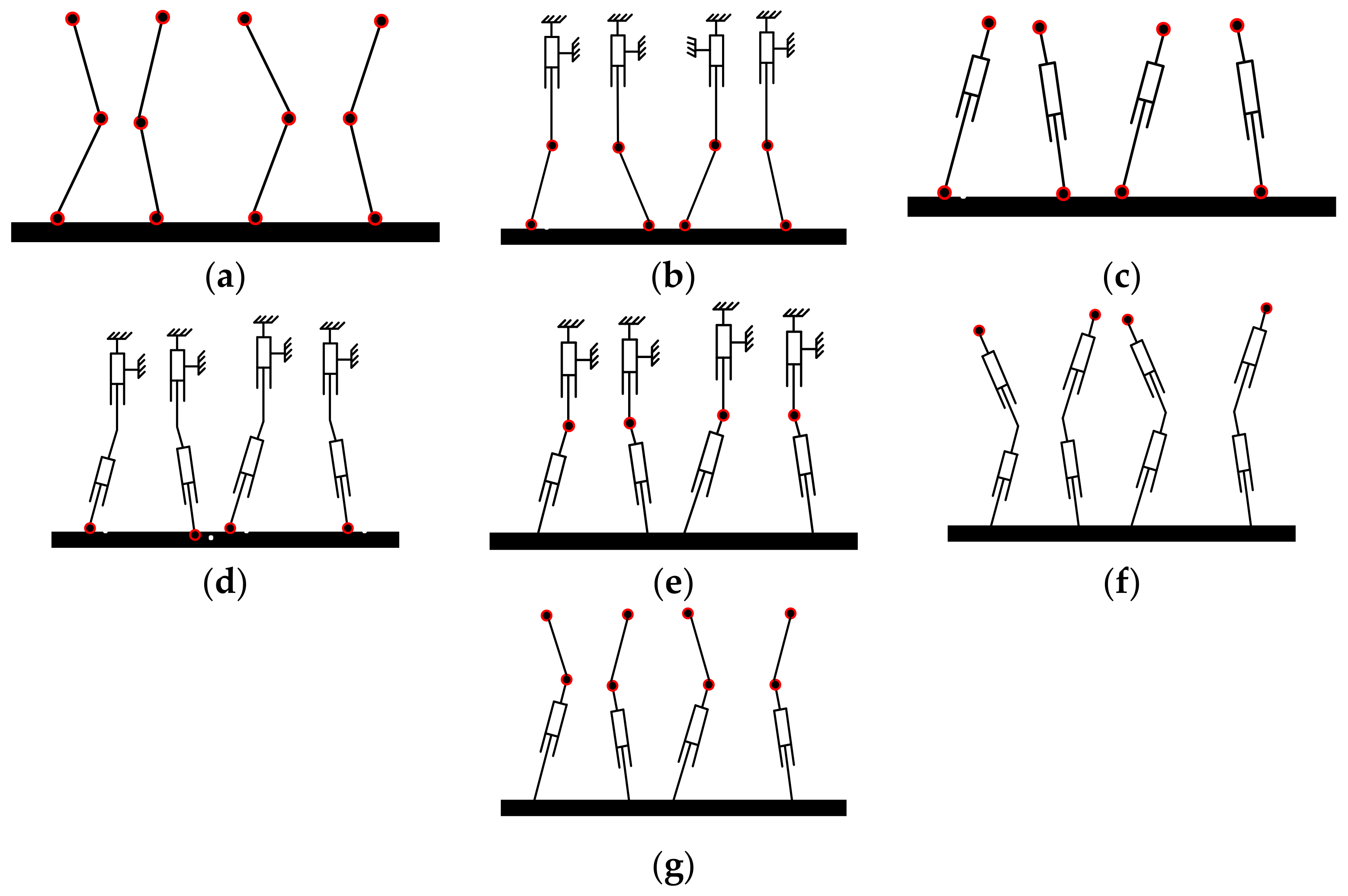
Analyzing the types of planar parallel part is a basic and essential procedure to obtain high stiffness for the support mechanism. Ensuring that at least three kinematic chains must have three DoFs and each kinematic chain must have an independent drive is a prerequisite. The planar kinematic joint includes a prismatic joint and a rotation joint. Thus, the types of driving chain can be expressed as RRR, PRR, RPR, PPR, PRP, RPP, and RRP without considering the suitable constraints. To increase stiffness and dexterity, the configurations are designed as redundantly actuated mechanisms. According to the types of driving chain, the parallel planar part can be composed as Figure 2 shows.

Given that the joint motion must be independent, the PPP type should be omitted. When exchanging the MP and fixed base of RRP, PRR, RPP, and PPR, an equivalent sequence should be considered. The requirement of large motion and high stiffness in the Y-direction should be considered. Thus, we select the P joint as the driving joint. Evidently, the RRR type should be omitted. The performance criterion must be considered while selecting the driving joint:

(a)

The driving joints must be distributed on each branch as evenly as possible.

(b)

The driving joints must be set on or near the fixed base and they must be prioritized.

(c)

The existence of a non-driving P joint should be avoided.

The criteria (a) and (b) are considered to reduce the moving mass and moment of inertia and to improve the dynamic performance of the mechanism. The driving joint setting on the MP should be avoided, and the RRP type may be omitted. In engineering, accuracy cannot be guaranteed when setting the non-driving of the P joint, and unless the noble guideway is used, the PPR, PRP, and RPP types can be omitted. On the basis of the aforementioned discussion, the PRR and RPR types are retained.

To further select the appropriate configuration for the parallel part with high stiffness, more attention must be paid to the remainder of the article to compare the two kinds of branch chain in terms of spatial stiffness.

3. Overall Jacobian Matrix

By using the closed vector method, achieving the spatial stiffness of a planar parallel mechanism is no longer satisfied. In this section, screw theory is used to calculate the overall Jacobian of the mechanism by analyzing the form of the active and constraint screws of each driving chain, which is the foundation of building the spatial stiffness model. We can obtain the joint instantaneous screws according to geometric relation of driving chains as shown in Figure 3.

The instantaneous velocity of MP can be represented as ${\widehat{\mathbf{S}}}_{\mathrm{p}}={\left[\begin{array}{cc}{\mathbf{v}}^{\mathrm{T}}& {\omega }^{\mathrm{T}}\end{array}\right]}^{\mathrm{T}}$; v and ω indicate the vector of translational velocity and vector of rotational velocity, respectively; the instantaneous screw of the MP can be represented through three linear un-correlation joint instantaneous screws.

$${\widehat{\mathbf{S}}}_{\mathrm{p}}={\dot{\mathrm{d}}}_{1i}{\widehat{\mathbf{\$}}}_{\mathrm{ta},1,i}+{\dot{\mathsf{\theta }}}_{2i}{\widehat{\mathbf{\$}}}_{\mathrm{ta},2,i}+{\dot{\mathsf{\theta }}}_{3i}{\widehat{\$}}_{3,ta,i},$$

(1)

where ${\widehat{\mathbf{\$}}}_{\mathrm{ta},k,i}$ denotes the kth joint instantaneous screw of the ith limb, k = 1−3, i indicates the driving chain number, ${\dot{\mathsf{\theta }}}_{ki}$ is the kth joint instantaneous rotational velocity of the ith limb, ${\dot{\mathrm{d}}}_{ki}$ represents the kth joint instantaneous translational velocity of the ith limb, ${\widehat{\mathbf{\$}}}_{\mathrm{ta}}$ is expressed in the Plücker ray coordinate, ${\widehat{\mathbf{\$}}}^1$ is the screw of each joint for PRR-type driving chain, ${\widehat{\mathbf{\$}}}^2$ is the screw of each joint for RPR-type driving chain, 0 represents a 3 × 1 zero vector, s_1,i is a unit vector along the P joint, q_i is a unit vector along the $\overrightarrow{BC}$, L_0,i is the length of BC, s_2,i and s_3,i are the unit vectors along the axis of R joints, b_i is the vector along $\overrightarrow{PB}$, “×” denotes cross-product.

$${\widehat{\mathbf{\$}}}_{\mathrm{ta},1,i}^1=\left(\begin{array}{c}{\mathbf{s}}_{1,i}\\ \mathbf{0}\end{array}\right),{\widehat{\mathbf{\$}}}_{\mathrm{ta},2,i}^1=\left(\begin{array}{c}({\mathbf{b}}_i+{\mathbf{q}}_i{\mathbf{L}}_{0,i})\times {\mathbf{s}}_{2,i}\\ {\mathbf{s}}_{2,i}\end{array}\right),{\widehat{\mathbf{\$}}}_{\mathrm{ta},3,i}^1=\left(\begin{array}{c}{\mathbf{b}}_i\times {\mathbf{s}}_{3,i}\\ {\mathbf{s}}_{3,i}\end{array}\right),$$

(2)

$${\widehat{\mathbf{\$}}}_{\mathrm{ta},1,i}^2=\left(\begin{array}{c}({\mathbf{b}}_i+{\mathbf{q}}_i{\mathbf{L}}_{0,i})\times {\mathbf{s}}_{2,i}\\ {\mathbf{s}}_{2,i}\end{array}\right),{\widehat{\mathbf{\$}}}_{\mathrm{ta},2,i}^2=\left(\begin{array}{c}{\mathbf{q}}_i\\ \mathbf{0}\end{array}\right),{\widehat{\mathbf{\$}}}_{\mathrm{ta},3,i}^2=\left(\begin{array}{c}{\mathbf{b}}_i\times {\mathbf{s}}_{3,i}\\ {\mathbf{s}}_{3,i}\end{array}\right),$$

(3)

where ${\widehat{\mathbf{\$}}}_{\mathrm{wc},k,i}$ denotes the kth reciprocal basis screw of the ith limb; n is a unit vector perpendicular to the P joint; the physical significance of ${\widehat{\mathbf{\$}}}_{\mathrm{wc},1,i}^1$ and ${\widehat{\mathbf{\$}}}_{\mathrm{wc},2,i}^1$ are constraint wrench around n and s_1,i, respectively; and ${\widehat{\mathbf{\$}}}_{\mathrm{wc},3,i}^1$ represents the constraint force along s_3,i.

$${\widehat{\mathbf{\$}}}_{\mathrm{wc},1,i}^1=\left(\begin{array}{c}\mathbf{0}\\ {\mathbf{n}}_i\end{array}\right),{\widehat{\mathbf{\$}}}_{\mathrm{wc},2,i}^1=\left(\begin{array}{c}\mathbf{0}\\ {\mathbf{s}}_{1,i}\end{array}\right),{\widehat{\mathbf{\$}}}_{\mathrm{wc},3,i}^1=\left(\begin{array}{c}{\mathbf{s}}_{3,i}\\ {\mathbf{b}}_{\mathbf{i}}\times {\mathbf{s}}_{3,i}\end{array}\right).$$

(4)

The physical significance of ${\widehat{\mathbf{\$}}}_{\mathrm{wc},1,i}^2$ and ${\widehat{\mathbf{\$}}}_{\mathrm{wc},2,i}^2$ are the constraint wrench around m_i and q_i, ${\mathbf{m}}_i={\mathbf{q}}_i\times {\mathbf{s}}_{1,i}$, and ${\widehat{\mathbf{\$}}}_{\mathrm{wc},3,i}^2$ represents the constraint force along s_3,i.

$${\widehat{\mathbf{\$}}}_{\mathrm{wc},1,i}^2=\left(\begin{array}{c}\mathbf{0}\\ {\mathbf{m}}_i\end{array}\right),{\widehat{\mathbf{\$}}}_{\mathrm{wc},2,i}^2=\left(\begin{array}{c}\mathbf{0}\\ {\mathbf{q}}_i\end{array}\right),{\widehat{\mathbf{\$}}}_{\mathrm{wc},3,i}^2=\left(\begin{array}{c}{\mathbf{s}}_{3,i}\\ {\mathbf{b}}_{\mathit{i}}\times {\mathbf{s}}_{3,i}\end{array}\right).$$

(5)

The dot product of Formulas (1)–(3) can be represented as follows:

$${\widehat{\mathbf{\$}}}_{\mathrm{wc},k,i}^{\mathrm{T}}{\hat{\mathbf{S}}}_{\mathrm{p}}=0.$$

(6)

Reorganized matrix form is given as follows:

$${\mathbf{J}}_c{\hat{\mathbf{S}}}_{\mathrm{p}}=\mathbf{0},$$

(7)

where, ${\mathbf{J}}_c^1$ and ${\mathbf{J}}_c^2$ are the constraint sub-matrixes of overall Jacobian.

$${\mathbf{J}}_c^1={\left[\begin{array}{c}\begin{array}{cc}\mathbf{0}& {\mathbf{n}}_1^{\mathrm{T}}\\ \mathbf{0}& {\mathbf{s}}_{1,1}^{\mathrm{T}}\\ {\mathbf{s}}_{2,1}^{\mathrm{T}}& {[{\mathbf{b}}_i\times {\mathbf{s}}_{3,1}]}^{\mathrm{T}}\end{array}\\ ⋮\\ \begin{array}{cc}\mathbf{0}& {\mathbf{n}}_i^{\mathrm{T}}\\ \mathbf{0}& {\mathbf{s}}_{1,i}^{\mathrm{T}}\\ {\mathbf{s}}_{2,i}^{\mathrm{T}}& {[{\mathbf{b}}_i\times {\mathbf{s}}_{3,i}]}^{\mathrm{T}}\end{array}\end{array}\right]}_{(3\times i)\times 6},{\mathbf{J}}_c^2={\left[\begin{array}{c}\begin{array}{cc}\mathbf{0}& {\mathbf{m}}_1^{\mathrm{T}}\\ \mathbf{0}& {\mathbf{q}}_1^{\mathrm{T}}\\ {\mathbf{s}}_{3,1}^{\mathrm{T}}& {[{\mathbf{b}}_i\times {\mathbf{s}}_{3,1}]}^{\mathrm{T}}\end{array}\\ ⋮\\ \begin{array}{cc}\mathbf{0}& {\mathbf{m}}_i^{\mathrm{T}}\\ \mathbf{0}& {\mathbf{q}}_i^{\mathrm{T}}\\ {\mathbf{s}}_{3,i}^{\mathrm{T}}& {[{\mathbf{b}}_i\times {\mathbf{s}}_{3,i}]}^{\mathrm{T}}\end{array}\end{array}\right]}_{(3\times i)\times 6}$$

(8)

When the input driving joint of each limb is locked, a reciprocal screw, which is reciprocated with other screws in a limb, ${\widehat{\mathbf{\$}}}_{\mathrm{wa},1,i}$ can be expressed in Equation (9),

$${\widehat{\mathbf{\$}}}_{\mathrm{wa},1,i}^1=\left(\begin{array}{c}{\mathbf{q}}_i\\ {\mathbf{r}}_i\times {\mathrm{q}}_i\end{array}\right),{\widehat{\mathbf{\$}}}_{\mathrm{wa},1,i}^2=\left(\begin{array}{c}{\mathbf{q}}_i\\ {\mathbf{r}}_i\times {\mathbf{q}}_i\end{array}\right),$$

(9)

where, ${\mathbf{r}}_i={\mathbf{b}}_i·\frac{\left|{\mathbf{b}}_i\times {\mathbf{q}}_i\right|}{\left|{\mathbf{b}}_i\right|\left.{\mathbf{q}}_i\right|}$, r_i is a vertical vector from origin P of the local reference frame to vector q_i. Take dot product of Equations (1) and (9),

$${\widehat{\mathbf{\$}}}_{\mathrm{wa},1,i}^{\mathrm{T}}{\mathbf{S}}_{\mathrm{p}}={\dot{\mathrm{d}}}_i.$$

(10)

Arranging Equation (9) into matrix form,

$$\begin{array}{c}{\mathbf{J}}_{\mathrm{a}}^1=\left[\begin{array}{cc}\frac{{\mathbf{q}}_i^{\mathrm{T}}}{{\mathbf{q}}_i^{\mathrm{T}}{\mathbf{s}}_1}& \frac{{({\mathbf{r}}_i\times {\mathbf{q}}_i)}^{\mathrm{T}}}{{\mathbf{q}}_i^{\mathrm{T}}{\mathbf{s}}_1}\end{array}\right]{}_{i\times 6},\\ {\mathbf{J}}_{\mathrm{a}}^2=\left[\begin{array}{cc}\frac{{\mathbf{q}}_i^{\mathrm{T}}}{{\mathbf{q}}_i^{\mathrm{T}}{\mathbf{s}}_1}& \frac{{({\mathbf{r}}_i\times {\mathbf{q}}_i)}^{\mathrm{T}}}{{\mathbf{q}}_i^{\mathrm{T}}{\mathbf{s}}_1}\end{array}\right]{}_{i\times 6}\end{array}$$

(11)

Remarkably, the velocity overall Jacobian J of the mechanism is expressed as

$$\mathbf{J}=\left[\begin{array}{c}{\mathbf{J}}_{\mathrm{a}}\\ {\mathbf{J}}_{\mathrm{c}}\end{array}\right]$$

(12)

By observing the overall Jacobian matrix, the first three rows of the matrix are dimensionless, and the last three rows are related to the position vector r. Unifying the dimensionless matrix is crucial, and the unified overall Jacobian matrix is given as follows:

$${\mathbf{J}}^1={\left[\begin{array}{c}\begin{array}{cc}\frac{{\mathbf{q}}_i^{\mathrm{T}}}{{\mathbf{q}}_i^{\mathrm{T}}{\mathbf{s}}_1}& \frac{{({\mathbf{r}}_i\times {\mathbf{q}}_i)}^{\mathrm{T}}}{{\mathbf{q}}_i^{\mathrm{T}}{\mathbf{s}}_1}\end{array}\\ ⋮\\ \begin{array}{cc}\mathbf{0}& {\mathbf{n}}_i^{\mathrm{T}}\\ \mathbf{0}& {\mathbf{s}}_{1,i}^{\mathrm{T}}\\ {\mathbf{s}}_{2,i}^{\mathrm{T}}& \frac{{[{\mathbf{b}}_i\times {\mathbf{s}}_{2,i}]}^{\mathrm{T}}}{\left|{\mathbf{b}}_i\right|}\end{array}\\ ⋮\end{array}\right]}_{(3\times i+i)\times 6},{\mathbf{J}}^2={\left[\begin{array}{c}\begin{array}{cc}\frac{{\mathbf{q}}_i^{\mathrm{T}}}{{\mathbf{q}}_i^{\mathrm{T}}{\mathbf{s}}_1}& \frac{{({\mathbf{r}}_i\times {\mathbf{q}}_i)}^{\mathrm{T}}}{{\mathbf{q}}_i^{\mathrm{T}}{\mathbf{s}}_1}\end{array}\\ ⋮\\ \begin{array}{cc}\mathbf{0}& {\mathbf{m}}_i^T\\ \mathbf{0}& {\mathbf{q}}_i^T\\ {\mathbf{s}}_{2,i}^T& \frac{{[{\mathbf{b}}_i\times {\mathbf{s}}_{2,i}]}^T}{\left|{\mathbf{b}}_i\right|}\end{array}\\ ⋮\end{array}\right]}_{(3\times i+i)\times 6}$$

(13)

4. Stiffness Model

The hydraulic motor is more adaptable to be the actuator because of its variable types of load. The PRR-type chain is shown in Figure 4a; the hydraulic motor only retains the DoF along the movement direction of the piston. The piston rod pushes the slider in which five constraint stiffnesses are provided by the guideway, as shown in Figure 4b. The RPR-type chain consists of one hydraulic motor and two rotational joints.

4.1. Active Stiffness

According to the active Jacobian analyzed above, it can be concluded that the active stiffness of each driving chain is the axial stiffness along $\overrightarrow{\mathrm{BC}}$. The active stiffness calculation methods of the two types are similar, but the stiffness of the guideway should be taken into account when calculating the active stiffness of PRR-type.

4.1.1. Active Stiffness of PRR Driving Chain

Actually, the active stiffness of the PRR type is along the direction of leg. In the process of force transmission of the PRR type, the stiffness of the hinge is neglected, thus the joint is in the force interaction position of the leg and slider shaft, as shown in Figure 5, and F is the axial force of the leg. According to Hooke’s law [29] and static analysis, we can acquire the following equations:

$$\begin{array}{l}{\mathrm{F}}_x=\mathrm{Fcos}(90-\mathsf{\theta })={\mathrm{k}}_x\Delta x,\\ {\mathrm{F}}_y=\mathrm{Fsin}(90-\mathsf{\theta })={\mathrm{k}}_y\Delta y,\\ \Delta \mathsf{\xi }=\sqrt{\mathsf{\Delta }{x}^2+\Delta y^2},\end{array}$$

where F is the unit force, $\Delta \mathsf{\xi }$ is the total deformation.

$${\mathrm{K}}_{\mathrm{v}}=\frac{\mathrm{F}}{\mathsf{\Delta }\mathsf{\xi }}=\frac{1}{\sqrt{{\left(\frac{\sin (90-\mathsf{\theta })}{{\mathrm{k}}_{\mathrm{y}}}\right)}^2+(\frac{\cos (90-\mathsf{\theta })}{{\mathrm{k}}_{\mathrm{x}}}{)}^2}},$$

(14)

$${\mathrm{k}}_{t,i}=\frac{1}{\sqrt{{(\frac{{\sin (90-\mathsf{\theta }}_i)}{{\mathrm{k}}_{a,i}})}^2+{(\frac{{\cos (90-\mathsf{\theta }}_i)}{{\mathrm{k}}_{gi,x}})}^2}}.$$

(15)

The tensile stiffness of the leg can be calculated by $k_{\mathrm{a}l,i}=\frac{\mathrm{E}{\mathrm{A}}_{\mathrm{L}}}{{\mathrm{L}}_{0,i}}$, where E denotes the elastic modulus [20], A_L represents the cross-sectional area of the leg, and L_0,i is the length of the leg. For the stiffness of hydraulic, k_a,i, see the details in Appendix A; the parameters of the hydraulic are presented in

Table A1. Physical parameters of hydraulic motor.

Parameter	Value	Parameter	Value
lab	0.450 m	E	2.1 × 105 N/m2
lbc	0.05 m	V1L	1.9 × 10−4 m3
R	0.014 m	V2L	1 × 10−4 m3
AAB	0.6154 m	b	0.032 m
ABC	1.9625 m	βe	1.8 × 109 N/m2
L1	0.026 m	A1	1.96 × 10−3 m2
L	0.38 m	A2	2.8 × 10−4 m2

in Appendix C. For the stiffness of the guideway in the direction perpendicular to movement of the slider, k_gi,x, see the details in Appendix B. The parameters of the guideway are presented in

Table A2. Physical parameters of guideway.

Parameter	Value	Parameter	Value
Le	0.0024 m	D	0.002 m
Lb	0.003 m	DW	0.004 m
bd	0.002 m	lt	0.058 m
Ls	0.126 m	Pz	0.00562 m
α	45°	Px	0.0172 m
Z0	26	n0	13

in Appendix C. Therefore, active stiffness is a serial spring system which is denoted by ${\mathrm{k}}_{\mathrm{act},i}^1$,

$${\mathrm{k}}_{\mathrm{act},i}^1={({\mathrm{k}}_{al,i}^{-1}+{\mathrm{k}}_{\mathrm{t},i}^{-1})}^{-1}.$$

(16)

4.1.2. Active Stiffness of RPR Driving Chain

According to the above analysis, the active stiffness of the RPR-type chains is along the movement of the piston rod. Thus, the active stiffness of RPR-type chains is the axial stiffness of the hydraulic motor.

$${\mathrm{k}}_{\mathrm{act},i}^2{=\mathrm{k}}_{a,i}$$

(17)

4.2. Constraint Stiffness

According to the constraint Jacobian analyzed above, the constraint stiffness of the two types of mechanism is composed of two kinds of torsional stiffness and a kind of tensile stiffness. The calculation method is to project the stiffness of the component on the corresponding vector direction in the constraint Jacobian. It needs to follow the spring superposition principle when the stiffness is composed of the different components.

4.2.1. Constraint Stiffness of PRR-Type Driving Chain

According to J_c, the constraint stiffness of the PRR type includes: the torsional stiffness around s_1,i the torsional stiffness around n_i, and the tensile stiffness along s_3,i [29].

The torsional stiffness around s_1,i is defined as $k_{con1,i}^1$, and k_tay denotes the torsional stiffness around s_1,i of the guideway, k_{lry, i} is the torsional stiffness around q_i of the leg at point C, I_p is a polar moment of inertia of the section.

$${\mathrm{k}}_{con1,i}^1={({\mathrm{k}}_{tay}^{-1}{+\mathrm{k}}_{lry,i,}^{-1})}^{-1},$$

(18)

$${\mathrm{k}}_{lry,i}=\frac{{\mathrm{GI}}_{\mathrm{p}}}{{\mathrm{L}}_{0,i}\cdot ({\mathbf{s}}_{1,i}^{\mathrm{T}}{\mathbf{q}}_i)},$$

(19)

where ${\mathrm{k}}_{con2,i}^1$ denotes the torsional stiffness around n_i, k_tax denotes the torsional stiffness around n_i of the guideway, k_{lrx, i} denotes the torsional stiffness around q_v,i of the leg at point C, q_v,i = q_i× s_3,i, and I_x denotes the moment of inertia.

$${\mathrm{k}}_{con2,i}^1={({\mathrm{k}}_{tax}^{-1}+{\mathrm{k}}_{lrx,i}^{-1})}^{-1},$$

(20)

$${\mathrm{k}}_{\mathrm{lrx},\mathrm{i}}=\frac{{\mathrm{EI}}_{\mathrm{x}}}{{\mathrm{L}}_{0,i}\cdot ({\mathbf{n}}_i^T{\mathbf{q}}_{\mathrm{v},i})}.$$

(21)

Tensile stiffness along s_3,i denotes ${\mathrm{k}}_{con3,i}^1$, k_tz is the torsional stiffness around s_3,i of the guideway, k_lz,i is the torsional stiffness around s_3,i of the leg at point C, I_z denotes the moment of inertia.

$${\mathrm{k}}_{con3,i}^1={({\mathrm{k}}_{tz}^{-1}+{\mathrm{k}}_{lz,i}^{-1})}^{-1},$$

(22)

$${\mathrm{k}}_{lz,i}=\frac{{3\mathrm{EI}}_{\mathrm{z}}}{{\mathrm{L}}_{0,i}^3}$$

(23)

4.2.2. Constraint Stiffness of RPR Driving Chain

In this research, we employ the mechanical model of a stepped cantilever beam to analyze the deformation under constraint stiffness from the perspective of material mechanics. l_cyl denotes length of a cylinder, l_rod is the piston rod sticking out of the cylinder part, and the constraint stiffness of type of RPR-driving chain can be expressed as follows [20,29]:

Torsional stiffness around m_i is defined as ${\mathrm{k}}_{con1,i}^2$,

$${\mathrm{k}}_{con1,i}^2=\mathrm{E}\left(\frac{l_{rod}}{{\mathrm{I}}_{\mathrm{x}1}}+\frac{l_{cyl}}{{\mathrm{I}}_{\mathrm{x}2}}\right)$$

(24)

Torsional stiffness around q_i is defined as ${\mathrm{k}}_{con2,i}^2$,

$${\mathrm{k}}_{con2,i}^2=\mathrm{G}\left(\frac{l_{rod}}{{\mathrm{I}}_{\mathrm{p}1}}+\frac{l_{cyl}}{{\mathrm{I}}_{\mathrm{p}2}}\right)$$

(25)

Tensile stiffness along s_3,i is defined as ${\mathrm{k}}_{con3,i}^2$,

$${\mathrm{k}}_{con3,i}^2=3\mathrm{E}/\left(\frac{l_{rod}^3}{{\mathrm{I}}_{\mathrm{z}1}}+\frac{l_{cyl}^3}{{\mathrm{I}}_{\mathrm{z}2}}\right)$$

(26)

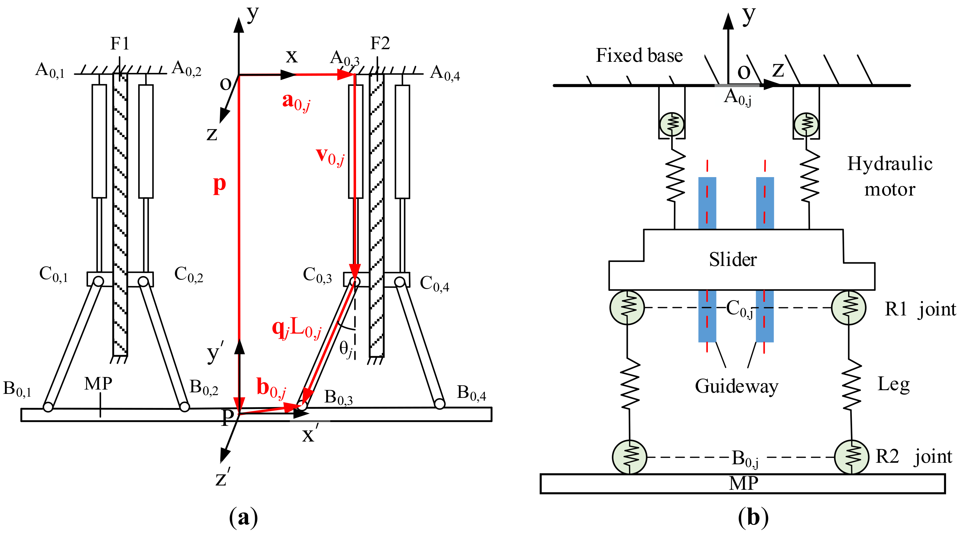
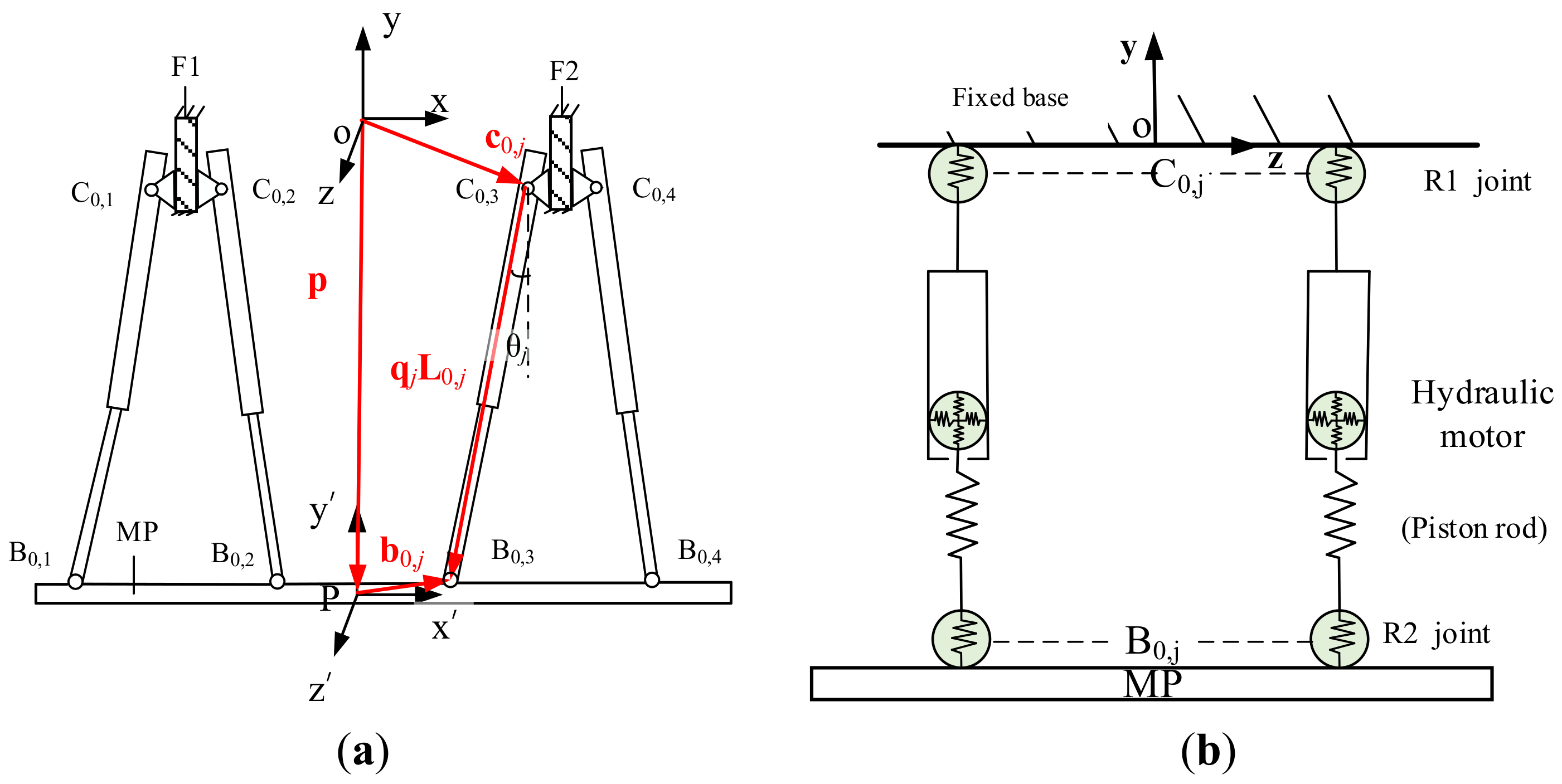
5. Mechanism Description and Inverse Position Analysis

According to the type discussion in Section 2, the planar part is set as a redundantly actuated parallel mechanism, and the purpose is to increase the active stiffness and enlarge the workspace. Besides, the driving force will be reduced through the effective optimization of driving force distribution. In order to increase constraint stiffness of the parallel part, each kinematic chain is set as an over-constrained mechanism. The kinematic model of the 4-(2PRR) mechanism is shown in Figure 6a; MP has the capability of x-direction translation, y-direction translation, and z-direction rotation in a planar movement space. The mechanism is composed of four kinematic chains, and each kinematic chain contains two driving chains. As shown in Figure 6b, each kinematic chain has two hydraulic motors used as the driving actuator, and these hydraulic motors push a slider to achieve the translation in the y-direction. The slider is connected with the leg through the hinge, and the two legs are also connected with the MP through the hinge.

In Figure 6a, F1 and F2 are fixed bases. F1 is parallel to F2. A fixed Cartesian reference frame, O-xyz, is assigned at the middle of the upper part of the F1 plate. Axis x, y, and z can be attached to point O in the fixed base; x-axis is perpendicular to F1, and y-axis parallel to F1. A moving frame, P-x′y′z′, is set at the centroid of the MP. In the x-y plane, A_0,j is the middle point of the connecting line between the two hydraulic motors of a kinematic chain, C_0,j is the middle point of the connecting line between the two rotating joints in a kinematic chain, and B_0,j is the middle point of the connecting line between the hinge points of the MP in a kinematic chain. For the convenient calculation of stiffness, we make the following agreements: n_i = [1,0,0] ^T, s_1,I = [0,1,0] ^T, s_2,I = s_3,I = [0,0,1] ^T.

Similarly, the kinematic model of the 4-(2RPR) mechanism is shown in Figure 7b. Only the form of driving chain is different, that is, the position of the MP and fixed base, and the reference frame is the same as those in the 4-(2RPR) mechanism. Hereinafter, we will use typeⅠ to stand for the 4-(2PRR) mechanism and type Ⅱ to stand for the 4-(2RPR) mechanism.

In Figure 6a, the single kinematic chain closed vector of type Ⅰ can be expressed as follows:

$$\begin{array}{l}\mathbf{p}+{\mathbf{B}}_{0,j}={\mathbf{h}}_{0,j}+{\mathbf{q}}_{0,j}{\mathbf{L}}_{0,j},{\mathbf{B}}_{0,j}=\mathbf{R}{\mathbf{b}}_{0,j},\\ {\mathbf{h}}_{0,j}={\mathbf{a}}_{0,j}+{\mathbf{\nu }}_{0,j},\end{array}$$

$${\mathbf{q}}_{0,j}{\mathbf{L}}_{0,j}={\mathbf{p}}_{0,j}+\mathbf{R}{\mathbf{b}}_{0,j}-{\mathbf{a}}_{0,j}-{\mathbf{v}}_{0,j},\hspace{1em}\hspace{1em}(j=1,2,3,4).$$

(27)

In Figure 7a, the single kinematic chain closed vector of type Ⅱ can be expressed as:

$${\mathbf{q}}_{0,j}{\mathbf{L}}_{0,j}={\mathbf{p}}_{0,j}+\mathbf{R}{\mathbf{b}}_{0,j}-{\mathbf{c}}_{0,j},\hspace{1em}(j=1,2,3,4)$$

(28)

In Equations (27) and (28), L_0,j is the length of the leg, j is the number of kinematic chain, q_0,j is the unit vector of the leg, R is the orientation matrix of the mobile platform, γ is the rotation angle of MP around the z-axis.

$$\mathrm{R}=\left[\begin{array}{ccc}\mathrm{c}\mathsf{\gamma }& -\mathrm{s}\mathsf{\gamma }& 0\\ \mathrm{s}\mathsf{\gamma }& \mathrm{c}\mathsf{\gamma }& 0\\ 0& 0& 1\end{array}\right]$$

The reachable workspace of the MP can be calculated according to the length of the leg, the constraint of the rotational angle, and the interference condition.

The geometric constraints of the mechanism are given as follows:

(1)

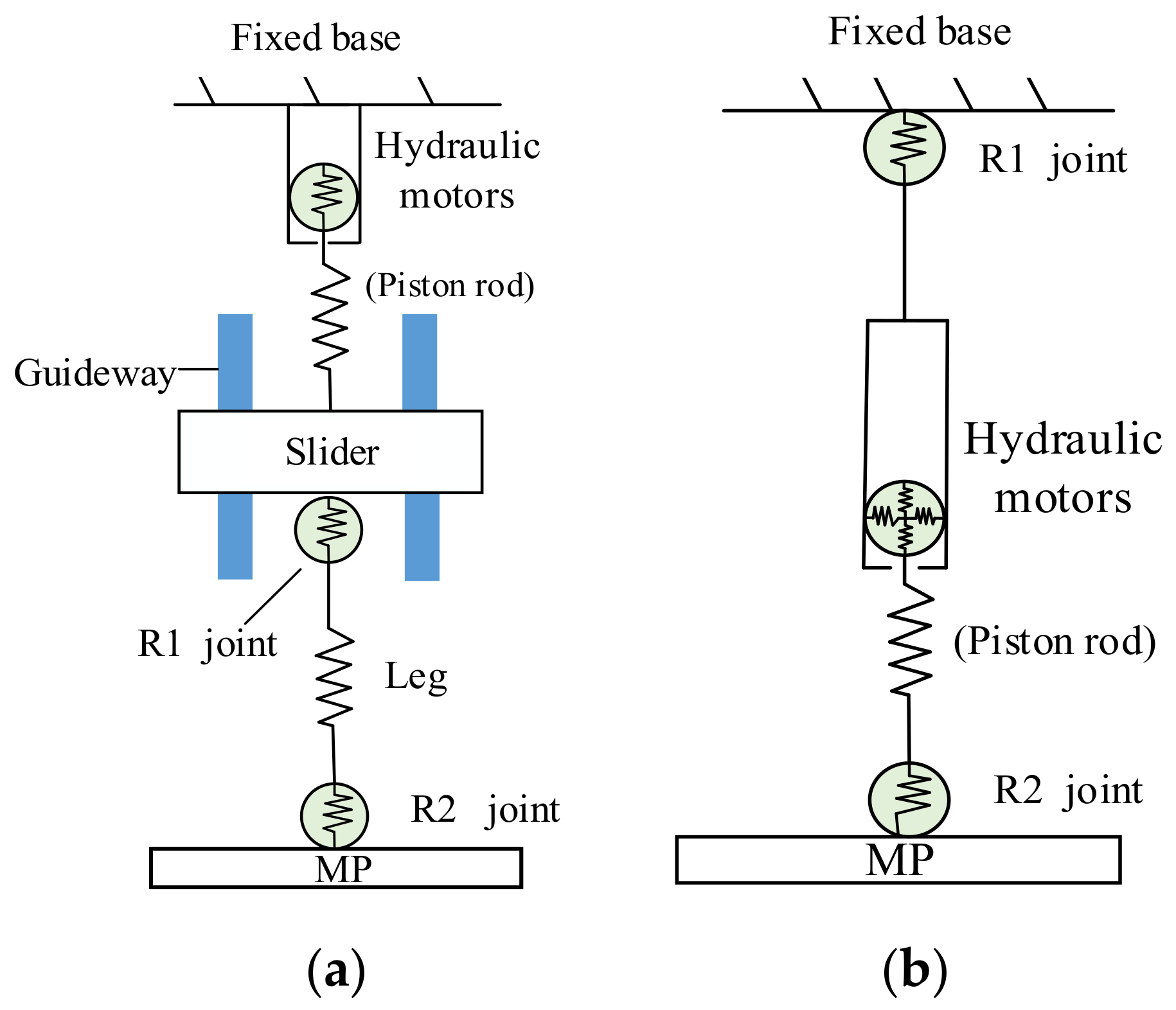
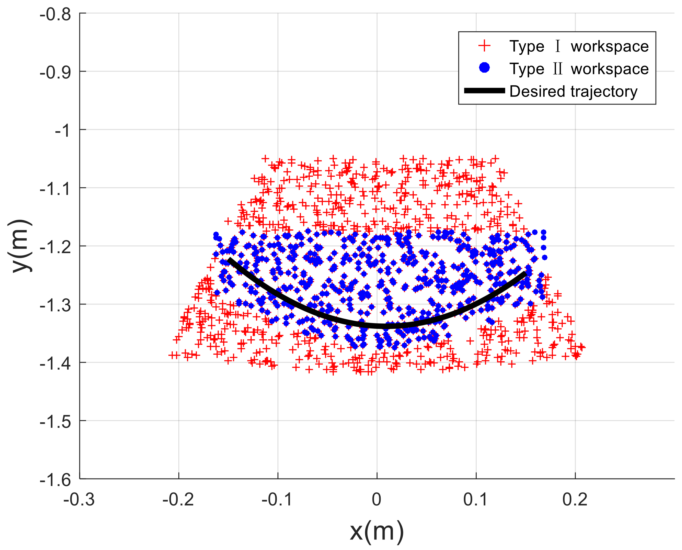
Stroke of active P joints. For each type of mechanism, the strokes of the hydraulic piston rod act as the actuator, which defines the workspace.

(2)

Rotational angle range of the R1 joint. To avoid the interference between links, the rotational angle range of the R1 joint should be considered:

$${\mathsf{\theta }}_j=\arccos \frac{{\mathbf{q}}_j·{\mathbf{s}}_1}{\left|{\mathbf{q}}_j\right|\left|{\mathbf{s}}_1\right|},\hspace{1em}(j=1,2,3,4).$$

(29)

(3)

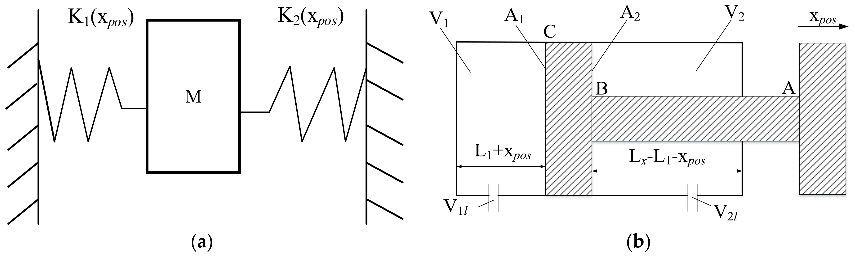
Interferences of MP between fixed base. As for type I, due to the particularity of the fixed base configuration and limitation for range of the P joint, the mobile platform will be restricted. As expressed in Equation (30), d₀ denotes the length of F1 and F2 in the y-direction, d_mp,j denotes the distance of MP to the fixed coordinate system in the y-direction.

$${\mathrm{d}}_0\le {\mathrm{d}}_{\mathrm{mp},j},\hspace{1em}(j=1,2,3,4)$$

(30)

To satisfy the requirements of the actual work area $\mathrm{x}\in (-0.17\mathrm{m},0.17\mathrm{m}),$$\mathrm{y}\in (-1.2\mathrm{m},-1.4\mathrm{m})$. In Figure 8, the MP workspace of type Ⅱ is larger than type Ⅰ, and it contains the workspace of type Ⅰ. This is related to the swing length of the rotating components (leg or hydraulic), and their workspaces are approximately x = 0 m symmetry.

6. Static Analysis and Stiffness Matrix Generation

Assuming that the MP is loaded from an external wrench ${\mathbf{F}}_{\mathrm{W}}={[\begin{array}{cc}{\mathbf{f}}^{\mathrm{T}}& {\mathbf{w}}^{\mathrm{T}}\end{array}]}^{\mathrm{T}}$, and it is expressed in the Plücker ray coordinate, $\mathbf{f}={[\begin{array}{ccc}{f}_x& f_y& f_z\end{array}]}^{\mathrm{T}}$ denotes the force vector, $\mathbf{w}={[\begin{array}{ccc}{w}_x& w_y& w_z\end{array}]}^{\mathrm{T}}$ is a wrench vector. Let f_a and f_c represent the reaction forces/torques of the actuators and constraints:

$${\mathbf{F}}_{\mathrm{W}}={\mathbf{J}}_{\mathrm{a}}^{\mathrm{T}}{\mathbf{f}}_{\mathrm{a}}+{\mathbf{J}}_{\mathrm{c}}^{\mathrm{T}}{\mathbf{f}}_{\mathrm{c}},$$

(31)

$${\mathbf{f}}_{\mathrm{a}}={\mathbf{k}}_a\Delta {\mathbf{x}}_{\mathrm{a}},$$

(32)

$${\mathbf{f}}_{\mathrm{c}}={\mathbf{k}}_c\Delta {\mathbf{x}}_{\mathrm{c}},$$

(33)

where k_a and k_c represent active and constraint stiffness, respectively; Δx_a and Δx_c are the displacements caused by the driving and constraint reactions of the limb, respectively. According to the principle of virtual work, we can achieve Equation (34), Δx_a = [Δx Δy Δz] denotes the linear displacement, Δx_c = [Δθ_x Δθ_y Δθ_z] denotes the angular displacement.

$${\mathbf{F}}_{\mathrm{W}}^{\mathrm{T}}\Delta \mathbf{x}={\mathbf{f}}_{\mathrm{a}}^{\mathrm{T}}\Delta {\mathbf{x}}_{\mathrm{a}}+{\mathbf{f}}_{\mathrm{c}}^{\mathrm{T}}\Delta {\mathbf{x}}_{\mathrm{c}}.$$

(34)

Gravity should be considered in external forces. F_E denotes the applied external force and F_G denotes the gravity of components:

$${\mathbf{F}}_{\mathrm{W}}={\mathbf{F}}_{\mathrm{E}}+{\mathbf{F}}_{\mathrm{G}},$$

(35)

$${\mathbf{F}}_{\mathrm{G}}^1={\mathbf{F}}_{\mathrm{G},\mathrm{S}}+{\mathbf{F}}_{\mathrm{G},\mathrm{L}}+{\mathbf{F}}_{\mathrm{G},\mathrm{M}},{\mathbf{F}}_{\mathrm{G}}^2={\mathbf{F}}_{\mathrm{G},\mathrm{H}}+{\mathbf{F}}_{\mathrm{G},\mathrm{M}}.$$

(36)

The applied external force ${\mathbf{F}}_{\mathrm{E}}={\left[\begin{array}{cc}{\mathbf{F}}_0^{\mathrm{T}}& {\mathbf{\tau }}_0^{\mathrm{T}}\end{array}\right]}^{\mathrm{T}}$ takes the position of the center of gravity as the action point, F_G,L is the gravity of the leg, F_G,S is the gravity of the slider, F_G,H is the gravity of the hydraulic cylinder, and F_G,M is the gravity of the MP.

$$\begin{array}{l}{\mathbf{F}}_{\mathrm{G},\mathrm{L}}={\displaystyle \sum _{i=1}^8{\mathrm{m}}_{\mathrm{L},i}\mathrm{g}\left[\begin{array}{c}{\mathbf{s}}_1\\ (\mathbf{R}{\mathbf{a}}_i-\frac{1}{2}{b}_i)\times {\mathbf{s}}_1\end{array}\right]},{\mathbf{F}}_{\mathrm{G},\mathrm{S}}={\displaystyle \sum _{j=1}^4{\mathrm{m}}_{\mathrm{S}}\mathrm{g}\left[\begin{array}{c}{\mathbf{s}}_1\\ (\mathbf{R}{\mathbf{a}}_j-{\mathbf{b}}_j)\times {\mathbf{s}}_1\end{array}\right]},{\mathbf{F}}_{\mathrm{G},\mathrm{H}}={\displaystyle \sum _{i=1}^8{\mathrm{m}}_{\mathrm{H}}\mathrm{g}\left[\begin{array}{c}{\mathbf{s}}_1\\ (\mathbf{R}{\mathbf{a}}_i-\frac{1}{2}{\mathbf{q}}_i{\mathrm{L}}_i)\times {\mathbf{s}}_1\end{array}\right]},\\ {\mathbf{F}}_{\mathrm{G},\mathrm{M}}={\mathrm{m}}_{\mathrm{M}}\mathrm{g}\left[\begin{array}{c}{\mathbf{s}}_1\\ \mathbf{0}\end{array}\right],\end{array}$$

where m_L denotes the mass of the leg, m_S denotes the mass of the slider, m_H denotes the mass of the hydraulic cylinder, m_M denotes the mass of the manipulator, and g denotes the acceleration of gravity; the parameters of mechanism are presented in

Table A3. Physical parameters of mechanism

Parameter	Value	Parameter	Value
mM	284 kg	mH	28.3 kg
mS	43.3 kg	L0,1/L0,2	0.392 m
mL,1	2.9 kg	L0,3/L0,4	0.443 m
mL,2	3.3 kg	L0,5/L0,6	0.482 m
mL,3	3.3 kg	L0,7/L0,8	0.4 m
mL,4	2.9 kg	g	9.8 m/s2

in Appendix C.

According to Hooke’s law [34], ΔX is the deformation in six directions, K is a 6 × 6 stiffness matrix.

$${\mathbf{F}}_{\mathrm{W}}=\mathbf{K}\Delta \mathbf{X}.$$

(37)

Taking Equation (34) into Equation (37) to achieve Equation (38), where $\overline{\mathbf{k}}=\mathrm{diag}({\mathbf{k}}_{\mathrm{a}},{\mathbf{k}}_{\mathrm{c}})$

$$\mathbf{K}={\mathbf{J}}^{\mathrm{T}}\overline{\mathbf{k}}\mathbf{J},$$

(38)

It should be noted that K is built in the moving frame, thereby transforming stiffness into the fixed frame to analyze the stiffness performance in the workspace.

$${\mathbf{K}}_{\mathrm{p}}={\mathbf{T}}^{\mathrm{T}}\mathbf{KT}$$

$$\mathbf{T}=\left[\begin{array}{cc}\mathbf{R}& -{\mathbf{l}}_{op}\times \\ \mathbf{0}& \mathbf{R}\end{array}\right]$$

[l_op×] is the skew symmetrical matrix relating to vector l_op from point P to point O. During the establishment of the stiffness matrix, the following assumptions are made:

(1)

No friction is observed between two contact joints.

(2)

No preload is observed on the MP.

(3)

The MP and the fixed platform are set as rigid bodies, and no deformation is observed.

(4)

Regardless of the antagonistic stiffness, the overall Jacobian matrix does not change caused by external force.

From Equation (38), we can obtain $\overline{\mathbf{k}}$ which can be expressed in a matrix form as 32 × 32 diagonal matrix.

$$\begin{array}{l}\overline{\mathbf{k}}={\mathrm{diag}(\mathrm{k}}_{\mathrm{act},1},{\mathrm{k}}_{\mathrm{act},2},{\mathrm{k}}_{\mathrm{act},3},{\mathrm{k}}_{\mathrm{act},4},{\mathrm{k}}_{\mathrm{act},5},{\mathrm{k}}_{\mathrm{act},6},{\mathrm{k}}_{\mathrm{act},7},{\mathrm{k}}_{\mathrm{act},8},\\ {\mathrm{k}}_{\mathrm{con}1,1},{\mathrm{k}}_{\mathrm{con}2,1},{\mathrm{k}}_{\mathrm{con}3,1},{\mathrm{k}}_{\mathrm{con}1,2},{\mathrm{k}}_{\mathrm{con}2,2},{\mathrm{k}}_{\mathrm{con}3,2},{\mathrm{k}}_{\mathrm{con}1,3},{\mathrm{k}}_{\mathrm{con}2,3},{\mathrm{k}}_{\mathrm{con}3,3},{\mathrm{k}}_{\mathrm{con}1,4},{\mathrm{k}}_{\mathrm{con}2,4},{\mathrm{k}}_{\mathrm{con}3,4},\\ {\mathrm{k}}_{\mathrm{con}1,5},{\mathrm{k}}_{\mathrm{con}2,5},{\mathrm{k}}_{\mathrm{con}3,5},{\mathrm{k}}_{\mathrm{con}1,6},{\mathrm{k}}_{\mathrm{con}2,6},{\mathrm{k}}_{\mathrm{con}3,6},{\mathrm{k}}_{\mathrm{con}1,7},{\mathrm{k}}_{\mathrm{con}2,7},{\mathrm{k}}_{\mathrm{con}3,7},{\mathrm{k}}_{\mathrm{con}1,8},{\mathrm{k}}_{\mathrm{con}2,8},{\mathrm{k}}_{\mathrm{con}3,8}).\end{array}$$

When the stiffness matrix of the parallel mechanism is achieved, the parallel mechanism should be evaluated in a virtual way. The reachable workspace of the two mechanisms is large enough compared with the actual work required. Thus, evaluating the stiffness along a specific trajectory is practical. According to the air flow direction of the experiment, the mechanism is affected by the force in the x-direction more strongly than in the other directions. Thus, the stiffness in the x-direction should be prioritized. The given trajectory in the x-direction ought to go throughout two workspaces and the trajectory equation is presented as follows:

$$\left\{\begin{array}{l}\mathrm{x}\left(\mathrm{t}\right)=-0.15+0.15\mathrm{t}\\ \mathrm{y}\left(\mathrm{t}\right)=1.338\sin (0.3957\mathrm{t}-1.9897)\\ \mathsf{\theta }\left(\mathrm{t}\right)=0\hspace{1em}\hspace{1em}\hspace{1em}\hspace{1em}\mathrm{t}\in [0,2]\end{array}\right.$$

(39)

To obtain the stiffness in all directions, the external F_E is applied to point P, and F_E is the unit force [1N, 1N, 1N, 1N·m, 1N·m, 1N·m] ^T. The deformation in all directions can be achieved from $\Delta {\mathbf{X}}_p={\mathbf{K}}_P^{-1}{\mathbf{F}}_W={\left[{\Delta }_{\rho x},{\Delta }_{\rho y},{\Delta }_{\rho z},{\Delta }_{ax},{\Delta }_{ay},{\Delta }_{az}\right]}^T$. In order to evaluate two types of mechanisms in the actual workspace, we use trajectory Equation (39) as the sub-workspace.

We used Δ_ρx, Δ_ρy, and Δ_ρz to denote the linear deformation along the x, y, and z directions in frame O-xyz, respectively, and employed Δ_ax, Δ_ay, and Δ_az to represent the angular deformations around the x, y, and z directions in frame O-xyz, respectively.

Figure 9 illustrates all directional deformation distributions of type Ⅰ in frame O-xyz. By carefully observing the cloud figure: (1) the maximum deformation occurred at the boundary position of the desired trajectory, and the minimum deformation occurred nearby x = 0 m, in which the linear deformation value has symmetrical distribution at approximately x = 0 m; (2) the variations of Δ_ρy and Δ_ρz, are associated with the y-axis, and the variations of Δ_ax, Δ_ay, and Δ_az mainly have relationship with the x-axis.

Figure 10 demonstrates all directional deformation distributions of type Ⅱ in frame O-xyz. Evidently, the symmetrical characteristic of the linear deformation distributions are similar to type Ⅰ. Notably, the increased levels of Δ_ρy, Δ_ρz, Δ_ay, and Δ_az have been associated with the decrease in the y-direction.

Generally, through the comparison of deformation value, we can find the stiffness of type Ⅰ is higher than that of type Ⅱ, except in the y-direction. Δ_ρy numerical value of the two types is relatively close. The reason has two aspects: (1) as for type Ⅰ, the active stiffness consists of axial stiffness of the leg and hydraulic; actually, the stiffness of the leg is an order of magnitude larger than the hydraulic, according to Equations (16) and (17), ${\mathrm{k}}_{\mathrm{act},i}^1$ is close to ${\mathrm{k}}_{\mathrm{act},i}^2$; (2) slider-guideway offers constraint stiffness for the driving chain instead of the hydraulic cylinder. As for type Ⅱ, the constraint stiffness depended on the hydraulic cylinder. From the deformation distribution values in each direction, we can find that type Ⅰ has a better stiffness characteristic.

The cloud figures can reflect the stiffness in six directions. From the overall Jacobian, we can find that the stiffness in the active directions are highly coupled, and the stiffness in the constraint directions are highly coupled, too. However, the active and constraint stiffnesses are fully decoupled. Therefore, investigating the influence of a certain parameter on active and constraint stiffness in the process of parameter optimization is beneficial.

Extracting the active and constraint stiffness from the overall stiffness is the essence of proposing the suitable indexes. For the convenience of stiffness expression, we use a compliance matrix instead of the stiffness matrix, in which ${\mathbf{K}}_{\mathrm{p}}^{-1}={\mathbf{C}}_{\mathrm{p}}$, Γ and Φ denote the selection matrix.

$${\mathbf{C}}_{\mathrm{p}}=\left[\begin{array}{cccccc}{\mathrm{c}}_{11}& {\mathrm{c}}_{12}& 0& 0& 0& {\mathrm{c}}_{16}\\ {\mathrm{c}}_{21}& {\mathrm{c}}_{22}& 0& 0& 0& {\mathrm{c}}_{26}\\ 0& 0& {\mathrm{c}}_{33}& {\mathrm{c}}_{34}& {\mathrm{c}}_{35}& 0\\ 0& 0& {\mathrm{c}}_{43}& {\mathrm{c}}_{44}& {\mathrm{c}}_{45}& 0\\ 0& 0& {\mathrm{c}}_{53}& {\mathrm{c}}_{54}& {\mathrm{c}}_{55}& 0\\ {\mathrm{c}}_{61}& {\mathrm{c}}_{62}& 0& 0& 0& {\mathrm{c}}_{66}\end{array}\right],$$

(40)

$$\mathbf{\Gamma }=\left[\begin{array}{cccccc}1& 0& 0& 0& 0& 0\\ 0& 1& 0& 0& 0& 0\\ 0& 0& 0& 0& 0& 1\end{array}\right],\mathbf{\Phi }=\left[\begin{array}{cccccc}0& 0& 1& 0& 0& 0\\ 0& 0& 0& 1& 0& 0\\ 0& 0& 0& 0& 1& 0\end{array}\right]$$

$${\mathbf{C}}_{\mathrm{act}}=\mathbf{\Gamma }{\mathbf{C}}_{\mathrm{p}}{\mathbf{\Gamma }}^{\mathrm{T}},{\mathbf{C}}_{\mathrm{con}}=\mathbf{\Phi }{\mathbf{C}}_p{\mathbf{\Phi }}^{\mathrm{T}}.$$

To eliminate dimensional effect, the characteristic length d_c is regarded as a constant, d_c is multiplied by the column of stiffness around the z-direction, and divided by the column of stiffness along the z-direction.

$${\mathbf{C}}_{act}=\left[\begin{array}{ccc}{\mathrm{c}}_{11}& {\mathrm{c}}_{12}& {\mathrm{c}}_{16}{\mathrm{d}}_{\mathrm{c}}\\ {\mathrm{c}}_{21}& {\mathrm{c}}_{22}& {\mathrm{c}}_{26}{\mathrm{d}}_{\mathrm{c}}\\ {\mathrm{c}}_{61}& {\mathrm{c}}_{62}& {\mathrm{c}}_{66}{\mathrm{d}}_{\mathrm{c}}\end{array}\right],{\mathbf{C}}_{con}=\left[\begin{array}{ccc}{\mathrm{c}}_{33}{/\mathrm{d}}_{\mathrm{c}}& {\mathrm{c}}_{34}& {\mathrm{c}}_{35}\\ {\mathrm{c}}_{43}{/\mathrm{d}}_{\mathrm{c}}& {\mathrm{c}}_{44}& {\mathrm{c}}_{45}\\ {\mathrm{c}}_{53}{/\mathrm{d}}_{\mathrm{c}}& {\mathrm{c}}_{54}& {\mathrm{c}}_{55}\end{array}\right]$$

The active stiffness index (ASI) can be defined in Equation (41), in which a higher value of ASI indicates a lower active stiffness characteristic, and W is a sub-workspace that is determined by the desired trajectory.

$$\mathrm{ASI}=\frac{{\displaystyle {\int }_{\mathrm{W}}\sqrt[3]{\det ({\mathbf{C}}_{act})}\mathrm{dW}}}{{\displaystyle {\int }_{\mathrm{W}}\mathrm{dW}}}$$

(41)

The constraint stiffness index (CSI) can be defined in Equation (42), in which a higher value of CSI indicates a lower constraint stiffness characteristic.

$$\mathrm{CSI}=\frac{{\displaystyle {\int }_{\mathrm{W}}\sqrt[3]{\det ({\mathbf{C}}_{con})}\mathrm{dW}}}{{\displaystyle {\int }_{\mathrm{W}}\mathrm{dW}}}$$

(42)

To move a step further to explore the parameter of actuator influence on active and constraint stiffness, we obtain the ASI and CSI varying curve through the range of hydraulic cylinder changes. From the index value of Figure 11, we can find that the active and constraint stiffnesses of typeⅠ is higher than those of type Ⅱ. When the range of hydraulic cylinder increases, the active stiffness of both types is decreased. We define the relative variation ratio of ASI and CSI as RVR, Max is the maximum value of indexes, Min is the minimum value of indexes. As for type Ⅰ, RVR of ASI is 23.5%, RVR of CSI is 9.4%. As for type Ⅱ, RVR of ASI is 263.5%, RVR of CSI is 18.1%. We can find that active stiffness is more affected than constraint stiffness, and type Ⅰ is less affected by the range of the hydraulic cylinder, especially on active stiffness.

$$\mathrm{RVR}=\frac{\mathrm{Max}-\mathrm{Min}}{\mathrm{Min}}\times 100\%$$

(43)

7. Discussion

This paper has calculated the spatial stiffness of the planar parallel mechanism and presented two novel stiffness indexes based on overall Jacobian. Compared with the previous research methods, it has the following advantages:

• Most studies only consider the stiffness in plane movement when analyzing the stiffness of the planar parallel mechanism. For example, the work [14] researched performance of three planar parallel manipulators, and finally a 3 × 3 stiffness matrix was achieved. However, the mechanism bears the force in six directions in the actual work. We build a stiffness model considering the constraint stiffness, which can reflect the actual stiffness characteristic of the mechanism.
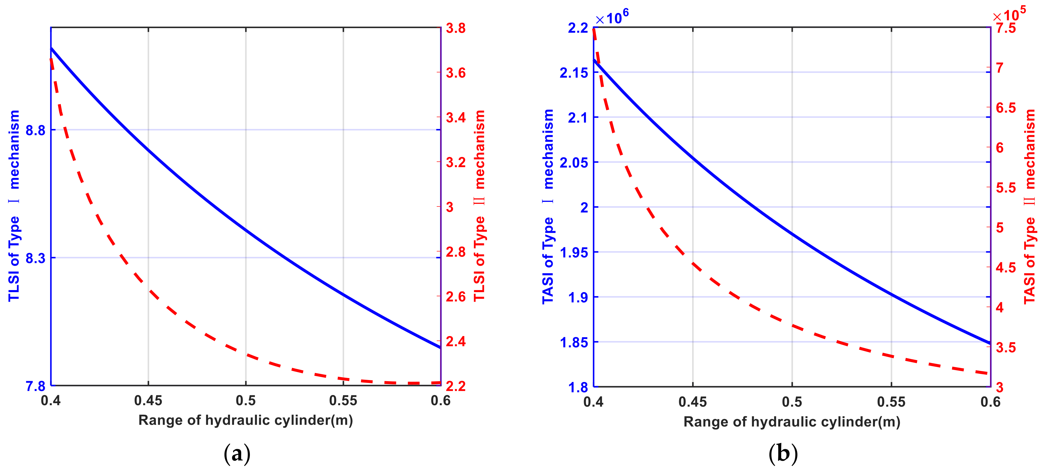
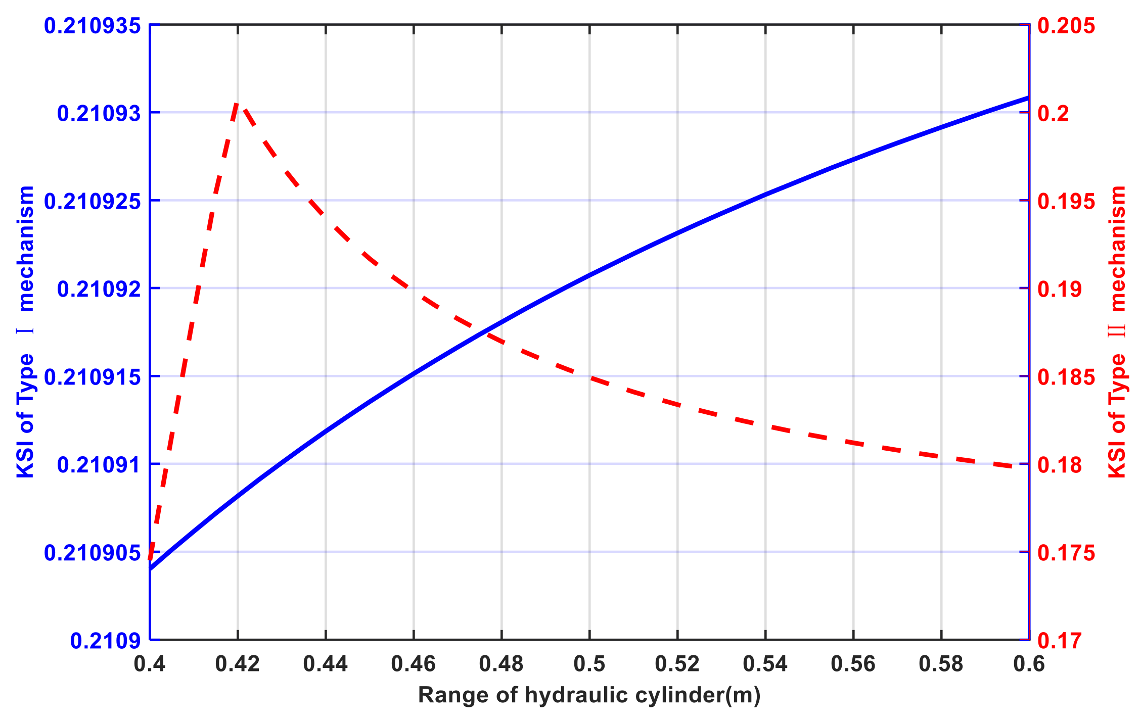
• Most of the existing stiffness indexes are focused on evaluating the isotropic characteristics of the mechanism and the ability to resist deformations. The total linear stiffness index (TLSI) and the total angular stiffness index (TASI) are separated to evaluate the ability of the mechanism to resist deformation in [40,41]. As shown in Equation (44), c_tt is the linear compliance element matrix, c_rr is the angular compliance element matrix. It can be found from Figure 12 that, with the increase of the hydraulic cylinder range, TLSI and TASI of the two types of mechanisms have the same decreasing trend. However, it is difficult to analyze the phenomenon from the theoretical formulas, and it brings obstacles for subsequent optimization of the component size. The stiffness index KSI was proposed in [34], which is a traditional mechanism stiffness evaluation method. As shown in Equation (45), λ_max, λ_min are the maximum and minimum eigenvalues of the stiffness matrix K_p, respectively This index reflects the isotropy of the mechanism geometry. From index values in Figure 13, we can find the hydraulic cylinder range has less effect on the KSI of the two mechanisms. This method lacks effective output parameter support for evaluating the dimensional characteristics of planar asymmetric mechanisms. When investigating the effect of the parameters on the stiffness in given directions, the proposed indexes are more clear explanations.

  $${\mathbf{C}}_p=\left[\begin{array}{cc}{\mathbf{c}}_{\mathrm{t}\mathrm{t}}& {\mathbf{c}}_{\mathrm{t}\mathrm{r}}\\ {\mathbf{c}}_{\mathrm{t}\mathrm{r}}^{\mathrm{T}}& {\mathbf{c}}_{\mathrm{r}\mathrm{r}}\end{array}\right],$$

  $$\mathrm{TLSI}=\frac{1}{\sqrt[3]{\det ({\mathbf{c}}_{\mathrm{t}\mathrm{t}})}},\mathrm{TASI}=\frac{1}{\sqrt[3]{\det ({\mathbf{c}}_{\mathrm{r}\mathrm{r}})}}.$$

  (44)

  $$\mathrm{KSI}=\sqrt{\frac{{\lambda }_{\min }}{{\lambda }_{\max }}}$$

  (45)

The application to two types of parallel planar part for a hybrid mechanism and some interesting results have been illustrated. We can find the type Ⅰ has better stiffness characteristics according to deformation distributions of the sub-workspace. In the constraint directions, the reason is that in the establishment of the constraint stiffness model, the guideway of type Ⅰ provides a part of the constrained stiffness. It can also be concluded from the ASI and CSI that type has better stiffness characteristics. It is worth noting that the influence of the hydraulic cylinder range on the active stiffness of type Ⅱ is more significant, and there exists a turning point when the length of the rod that sticks out of the hydraulic cylinder is 0.485 m. This may be a noteworthy research direction for stiffness optimization in future work.

In future work, the proposed indexes will be applied to the spatial parallel mechanism, and multi-objective optimization may be researched based on ASI and CSI.

References

1. Pereira, J.D. Wind Tunnels: Aerodynamics, Model and Experiments; Nova Science Publishers, Inc.: Hauppauge, NY, USA, 2011; ISBN 9781619423299. [Google Scholar]
2. Portman, V.; Sandler, B.Z.; Chapsky, V.; Zilberman, I. A 6-DOF isotropic measuring system for force and torque components of drag for use in wind tunnels: IIInnovative design. Int. J. Mech. Mater. Des. 2009, 5, 337–352. [Google Scholar] [CrossRef]
3. Lafourcade, P.; Llibre, M. First steps toward a sketch-based design methodology for wire-driven manipulators. In Proceedings of the IEEE/ASME International Conference on Advanced Intelligent Mechatronics, Kobe, Japan, 20–24 July 2003; AIM: Townsville, Australia, 2003; Volume 1, pp. 143–148. [Google Scholar]
4. Yangwen, X.; Qi, L.; Yaqing, Z.; Bin, L. Model aerodynamic tests with a wire-driven parallel suspension system in low-speed wind tunnel. Chin. J. Aeronaut. 2010, 23, 393–400. [Google Scholar] [CrossRef] [Green Version]
5. Johnson, W.G.; Dress, D.A. 13-Inch Magnetic Suspension and Balance System Wind Tunnel; NASA Technical Memorandum; NASA: Hampton, VA, USA, 1989.
6. Rein, M.; Höhler, G.; Schütte, A.; Bergmann, A.; Löser, T. Ground-based simulation of complex maneuvers of a delta-wing aircraft. In Proceedings of the AIAA Aerodynamic Measurement Technology & Ground Testing Conference, San Francisco, CA, USA, 5–8 June 2006; DLR: Oberpfaffenhofen, Germany, 2006; pp. 2–6. [Google Scholar]
7. Bergmann, A.; Huebner, A.; Loeser, T. Experimental and numerical 1research on the aerodynamics of unsteady moving aircraft. Prog. Aerosp. Sci. 2008, 44, 121–137. [Google Scholar] [CrossRef]
8. Honegger, M.; Codourey, A.; Burdet, E. Adaptive control of the hexaglide, a 6 dof parallel manipulator. In Proceedings of the IEEE International Conference on Robotics and Automation, Albuquerque, NM, USA, 25 April 1997; Volume 1, pp. 543–548. [Google Scholar]
9. Guigue, A.; Ahmadi, M.; Tang, F.C. On the kinematic analysis and design of a redundant manipulator for a Captive Trajectory Simulation system (CTS). In Proceedings of the 2006 Canadian Conference on Electrical and Computer Engineering, Ottawa, ON, Canada, 7–10 May 2006; pp. 1514–1517. [Google Scholar] [CrossRef]
10. Jiang, L.Y.; Tang, F.C.; Benmeddour, A.; Fortin, F. Sting effects on store captive loads. In Proceedings of the 39th Aerospace Sciences Meeting and Exhibit, Ottawa, QC, Canada, 8–11 January 2001; AIAA: Reno, NV, USA, 2001; pp. 6–8. [Google Scholar]
11. Bergmann, A. Modern wind tunnel techniques for unsteady testing-Development of dynamic test rigs. Notes Numer. Fluid Mech. Multidiscip. Des. 2009, 102, 59–77. [Google Scholar] [CrossRef]
12. Geng, X.; Shi, Z.; Cheng, K.; Li, L. A new hybrid mechanism for dynamic wind tunnel test of high maneuverable air vehicle. Proc. Inst. Mech. Eng. Part G J. Aerosp. Eng. 2016, 230, 1964–1974. [Google Scholar] [CrossRef]
13. Zhang, D.; Xu, Y.; Yao, J.; Hu, B.; Zhao, Y. Kinematics, dynamics and stiffness analysis of a novel 3-DOF kinematically/actuation redundant planar parallel mechanism. Mech. Mach. Theory 2017, 116, 203–219. [Google Scholar] [CrossRef]
14. Wu, J.; Wang, J.; Wang, L.; You, Z. Performance comparison of three planar 3-DOF parallel manipulators with 4-RRR, 3-RRR and 2-RRR structures. Mechatronics 2010, 20, 510–517. [Google Scholar] [CrossRef]
15. Arsenault, M.; Boudreau, R. Synthesis of planar parallel mechanisms while considering workspace, dexterity, stiffness and singularity avoidance. J. Mech. Des. Trans. ASME 2006, 128, 69–78. [Google Scholar] [CrossRef]
16. Gallant, M.; Boudreau, R. The synthesis of planar parallel manipulators with prismatic joints for an optimal, singularity-free workspace. J. Robot. Syst. 2002, 19, 13–24. [Google Scholar] [CrossRef]
17. Wu, G.; Bai, S.; Kepler, J. Stiffness characterization of a 3-PPR planar parallel manipulator with actuation compliance. Proc. Inst. Mech. Eng. Part C J. Mech. Eng. Sci. 2015, 229, 2291–2302. [Google Scholar] [CrossRef]
18. Klimchik, A.; Chablat, D.; Pashkevich, A. Stiffness modeling for perfect and non-perfect parallel manipulators under internal and external loadings. Mech. Mach. Theory 2014, 79, 1–28. [Google Scholar] [CrossRef] [Green Version]
19. Pashkevich, A.; Klimchik, A.; Chablat, D. Enhanced stiffness modeling of manipulators with passive joints. Mech. Mach. Theory 2011, 46, 662–679. [Google Scholar] [CrossRef] [Green Version]
20. Pashkevich, A.; Chablat, D.; Wenger, P. Stiffness analysis of overconstrained parallel manipulators. Mech. Mach. Theory 2009, 44, 966–982. [Google Scholar] [CrossRef] [Green Version]
21. Deblaise, D.; Hernot, X.; Maurine, P. Asystematic analytical method for PKM Stiffness Matrix Calculation. In Proceedings of the 2006 IEEE International Conference on Robotics and Automation, Orlando, FL, USA, 15–19 May 2006; pp. 4213–4219. [Google Scholar]
22. Wu, J.; Wang, J.; Wang, L.; Li, T.; You, Z. Study on the stiffness of a 5-DOF hybrid machine tool with actuation redundancy. Mech. Mach. Theory 2009, 44, 289–305. [Google Scholar] [CrossRef]
23. Zhang, J.; Zhao, Y.; Jin, Y. Kinetostatic-model-based stiffness analysis of Exechon PKM. Robot. Comput. Integr. Manuf. 2016, 37, 208–220. [Google Scholar] [CrossRef] [Green Version]
24. Cao, W.A.; Ding, H. A method for stiffness modeling of 3R2T overconstrained parallel robotic mechanisms based on screw theory and strain energy. Precis. Eng. 2018, 51, 10–29. [Google Scholar] [CrossRef]
25. Yang, C.; Li, Q.; Chen, Q.; Xu, L. Elastostatic stiffness modeling of overconstrained parallel manipulators. Mech. Mach. Theory 2018, 122, 58–74. [Google Scholar] [CrossRef]
26. Cao, W.A.; Yang, D.; Ding, H. A method for stiffness analysis of overconstrained parallel robotic mechanisms with Scara motion. Robot. Comput. Integr. Manuf. 2018, 49, 426–435. [Google Scholar] [CrossRef]
27. Raoofian, A.; Taghvaeipour, A.; Kamali, A. On the stiffness analysis of robotic manipulators and calculation of stiffness indices. Mech. Mach. Theory 2018, 130, 382–402. [Google Scholar] [CrossRef]
28. Yan, S.J.; Ong, S.K.; Nee, A.Y.C. Stiffness analysis of parallelogram-type parallel manipulators using a strain energy method. Robot. Comput. Integr. Manuf. 2016, 37, 13–22. [Google Scholar] [CrossRef]
29. Li, Y.; Xu, Q. Stiffness analysis for a 3-PUU parallel kinematic machine. Mech. Mach. Theory 2008, 43, 186–200. [Google Scholar] [CrossRef]
30. Lian, B.; Sun, T.; Song, Y.; Jin, Y.; Price, M. Stiffness analysis and experiment of a novel 5-DoF parallel kinematic machine considering gravitational effects. Int. J. Mach. Tools Manuf. 2015, 95, 82–96. [Google Scholar] [CrossRef] [Green Version]
31. Sun, T.; Lian, B.; Song, Y. Stiffness analysis of a 2-DoF over-constrained RPM with an articulated traveling platform. Mech. Mach. Theory 2016, 96, 165–178. [Google Scholar] [CrossRef]
32. Joshi, S.A.; Tsai, L.W. Jacobian analysis of limited-DOF parallel manipulators. J. Mech. Des. Trans. ASME 2002, 124, 254–258. [Google Scholar] [CrossRef]
33. Ding, J.; Wang, C.; Wu, H. Accuracy analysis of redundantly actuated and overconstrained parallel mechanisms with actuation errors. J. Mech. Robot. 2018, 10, 1–7. [Google Scholar] [CrossRef]
34. Gosselin, C. Stiffness mapping for parallel manipulators. IEEE Trans. Robot. Autom. 1990, 6, 377–382. [Google Scholar] [CrossRef]
35. Bhattacharya, S.; Hatwal, H.; Ghosh, A. On the Optimum Design of Stewart Platform Type Parallel Manipulators. Robotica 1995, 13, 133–140. [Google Scholar] [CrossRef]
36. Chiacchio, P.; Chiaverini, S.; Sciavicco, L.; Siciliano, B. Global Task Space Manipulability Ellipsoids for Multiple-Arm Systems. IEEE Trans. Robot. Autom. 1991, 7, 678–685. [Google Scholar] [CrossRef]
37. Asada, H. A geometrical representation of manipulator dynamics and its application to arm design. J. Dyn. Syst. Meas. Control. Trans. ASME 1983, 105, 131–142. [Google Scholar] [CrossRef]
38. Huang, S.; Schimmels, J.M. The bounds and realization of spatial stiffnesses achieved with simple springs connected in parallel. IEEE Trans. Robot. Autom. 1998, 14, 466–475. [Google Scholar] [CrossRef] [Green Version]
39. Huang, S.; Schimmels, J.M. The eigenscrew decomposition of spatial stiffness matrices. IEEE Trans. Robot. Autom. 2000, 16, 146–156. [Google Scholar] [CrossRef]
40. Chen, C.; Peng, F.; Yan, R.; Li, Y.; Wei, D.; Fan, Z.; Tang, X.; Zhu, Z. Stiffness performance index based posture and feed orientation optimization in robotic milling process. Robot. Comput. Integr. Manuf. 2019, 55, 29–40. [Google Scholar] [CrossRef]
41. Guo, Y.; Dong, H.; Ke, Y. Stiffness-oriented posture optimization in robotic machining applications. Robot. Comput. Integr. Manuf. 2015, 35, 69–76. [Google Scholar] [CrossRef]
42. Li, M.; Wu, H.; Handroos, H. Static stiffness modeling of a novel hybrid redundant robot machine. Fusion Eng. Des. 2011, 86, 1838–1842. [Google Scholar] [CrossRef]
43. Liu, S. The Mechanical Analysis of Roller Linear Guideway; Huazhong University of Science and Technology: Wuhan, China, 2011. [Google Scholar]
Figure 1. Aircraft model support system in the wind tunnel.
Applsci 10 06342 g001
Figure 2. Types of 3-DoF planar parallel part. (a) 4-RRR planar parallel part; (b) 4-PRR planar parallel part; (c) 4-RPR planar parallel part; (d) 4-PPR planar parallel part; (e) 4-PRP planar parallel part; (f) 4-RPP planar parallel part; (g) 4-RRP planar parallel part.
Applsci 10 06342 g002
Figure 3. Two types of driving chain. (a) PRR-type driving chain; (b) RPR-type driving chain.
Applsci 10 06342 g003
Figure 4. Topology structure of driving chain. (a) Topology structure of PRR driving chain; (b) topology structure of RPR driving chain.
Applsci 10 06342 g004
Figure 5. Static analysis at R1 joint.
Applsci 10 06342 g005
Figure 6. Kinematic models of 4-(2PRR) parallel planar mechanism. (a) Kinematic model of the 4-(2PRR) redundant parallel manipulator; (b) topology structure of 4-(2PRR) kinematic chain.
Applsci 10 06342 g006
Figure 7. Kinematic models of 4-(2RPR) parallel planar mechanism. (a) Kinematic model of the 4-(2RPR) redundant parallel manipulator; (b) topology structure of 4-(2RPR) kinematic chain.
Applsci 10 06342 g007
Figure 8. Reachable workspace of MP.
Applsci 10 06342 g008
Figure 9. Deformation distributions of the mechanism in the sub-workspace of type I. (a) Linear deformation distribution in x direction of type I; (b) Linear deformation distribution in y direction of type I; (c) Linear deformation distribution in z direction of type I; (d) Angular deformation distribution in x direction of type I; (e) Angular deformation distribution in y direction of type I; (f) Angular deformation distribution in z direction of type I.
Applsci 10 06342 g009
Figure 10. Deformation distributions of the mechanism in the sub-workspace of type II. (a) Linear deformation distribution in x direction of type II; (b) Linear deformation distribution in y direction of type II; (c) Linear deformation distribution in z direction of type II; (d) Angular deformation distribution in x direction of type II; (e) Angular deformation distribution in y direction of type II; (f) Angular deformation distribution in z direction of type II.
Applsci 10 06342 g010
Figure 11. ASI and CSI variation caused by a range of hydraulic cylinder. (a) ASI index variation of two type mechanisms; (b) CSI index variation of two type mechanisms; The blue solid line stands for index of type Ⅰ mechanism, the red dashed line stands for index of type Ⅱ mechanism.
Applsci 10 06342 g011
Figure 12. TLSI and TASI variation caused by a range of hydraulic cylinder. (a) TLSI index variation of two type mechanisms; (b) TASI index variation of two type mechanisms; The blue solid line stands for index of typeⅠ mechanism, the red dashed line stands for index of type Ⅱ mechanism.
Applsci 10 06342 g012
Figure 13. KSI variation caused by a range of hydraulic cylinder. The blue solid line stands for index of type Ⅰ mechanism, the red dashed line stands for index of type Ⅱ mechanism.
Applsci 10 06342 g013