Article

News Classification for Identifying Traffic Incident Points in a Spanish-Speaking Country: A Real-World Case Study of Class Imbalance Learning

by
Gilberto Rivera
,
Rogelio Florencia
*,
Vicente García
,
Alejandro Ruiz
and
J. Patricia Sánchez-Solís
Departamento de Eléctrica y Computación, División Multidisciplinaria de Ciudad Universitaria, Universidad Autónoma de Ciudad Juárez, Av. José de Jesús Macías Delgado #18100, Cd. Juárez 32000, Chihuahua, Mexico
*
Author to whom correspondence should be addressed.
Appl. Sci. 2020, 10(18), 6253; https://doi.org/10.3390/app10186253
Submission received: 30 June 2020 / Revised: 25 August 2020 / Accepted: 29 August 2020 / Published: 9 September 2020

Abstract

:
‘El Diario de Juárez’ is a local newspaper in a city of 1.5 million Spanish-speaking inhabitants that publishes texts of which citizens read them on both a website and an RSS (Really Simple Syndication) service. This research applies natural-language-processing and machine-learning algorithms to the news provided by the RSS service in order to classify them based on whether they are about a traffic incident or not, with the final intention of notifying citizens where such accidents occur. The classification process explores the bag-of-words technique with five learners (Classification and Regression Tree (CART), Naïve Bayes, kNN, Random Forest, and Support Vector Machine (SVM)) on a class-imbalanced benchmark; this challenging issue is dealt with via five sampling algorithms: synthetic minority oversampling technique (SMOTE), borderline SMOTE, adaptive synthetic sampling, random oversampling, and random undersampling. Consequently, our final classifier reaches a sensitivity of 0.86 and an area under the precision-recall curve of 0.86, which is an acceptable performance when considering the complexity of analyzing unstructured texts in Spanish.

1. Introduction

Nowadays, most of the people across the world live in urban areas, and the UN expects this population to increase dramatically in the coming three decades. The leading causes are (1) the shift in the residence of people from rural communities to urban ones and (2) the growth of the whole population, adding 2.5 billion people to cities [1]. This trend is particularly marked in the case of in-development regions. As a precaution from the consequences of such a prospect, the Director of the Population Division of the UN stated that
Managing urban areas has become one of the most important development challenges of the 21st century. Our success or failure in building sustainable cities will be a major factor in the success of the post-2015 UN development agenda [2].
Accordingly, many of the low and middle-income countries will face critical challenges arising from the needs of their cities, including security, employment, health care, energy supply, education, housing, and transportation. As urbanization intensifies, sustainable development depends on the successful management of—often scarce—urban resources.
Here, Information and Communication Technology (ICT) is mainly a matter of interest. During the last two decades, urban structures have become more digital and information-based, and there has been a decisive change in the living environment of citizens. However, they must be capable of further advances as ICT innovations emerge. These cities must gain a competitive edge by adopting new technologies, such as the Internet of Things (IoT), cloud computing, big data, and mobile computing (cf. [3]).
The future so-called ‘large’ and ‘mega’ cities must evolve towards sustainability to provide a satisfactory standard of living for their inhabitants. In this context, they must reach the longed-for status of ‘Smart City’ and ‘Knowledge Society’. According to the Smart Cities Council [4], “a smart city uses information and communications technology (ICT) to enhance livability, workability, and sustainability”.
Williams [5] prefers to use the concept ‘Smart Community’ (SC) because of the lack of a globally unified notion of what a city is (in terms of population, physical size, geographical location, among others). Accordingly, an SC is any community—regardless of its degree of urbanization—that responds efficiently and rapidly to the population’s emerging needs. It is supposed to:
  • Improve operations that impact its quality of life (e.g., economic vitality, education, employment, environmental footprint, health care, power supply, safety, and transportation).
  • Enable a shared understanding of what is happening in the ‘city’.
  • Engage both citizens and (private and public) organizations.
In this paper, we present a real-world web application that directly impacts the afore-mentioned Point 2. The case study occurs in Mexico, specifically in Ciudad Juárez (in the Mexican State of Chihuahua). Mexico is in the top five of countries with the fastest-growing urbanization degree [1]; and, additionally, Ciudad Juárez is the fifth largest city in that country and it is expected to become a ‘large’ city in the following years, according to the current UN’s criteria. With a fast-increasing population, this city must provide structures that rapidly broadcast knowledge among all of the members of its community.
This fact brings to light that Ciudad Juárez should evolve towards an SC urgently. In this sense, the case study falls into the UN’s priorities. However, much work must be done to offer acceptable living conditions. The inception of this study arises from the need to notify citizens about traffic accidents. It consists of the following tasks:
  • get a corpus of news published by the local newspaper through an RSS (Really Simple Syndication) feed,
  • get a vector characterization based on the well-known Bag-of-Words (BoW) representation [6],
  • select features through a mutual information-based method,
  • train a supervised-learning model,
  • classify online news reports in real-time; the interest is in the ‘traffic accident’ class,
  • process the text of the RSS reports to retrieve the location where the accidents happened, and
  • notify users about the events on a map.
Two fields of Artificial Intelligence converge to solve this problem: Natural Language Processing (NLP) and machine learning. However, the presence of class imbalance is one of the most challenging issues to address Points 4 and 5 satisfactorily. According to the scientific literature [7,8,9,10], this issue often degrades machine learning approaches, which skews the classification capacity in favor of the most crowded class.
On top of that, most of the studies in the literature are highly focused on the English language. As far as we know, a few studies are researching about classifying Spanish news with class imbalance, even though:
  • Latin-America is the second most urbanized region of the world [1],
  • Spanish is the second most spoken language [11], and
  • Spanish is the third most used language on the Web [12].
However, communities of native Spanish speakers also have the needs that entail the successful application of NLP to take a further step towards becoming an SC. In this regard, our proposal contributes by addressing one of these demanding needs.
The present document is structured, as follows: Section 2 contains the scientific basis for developing our proposal; Section 3 reviews the contributions of relevant studies that address this problem; Section 4 provides the algorithm and architecture of our project, giving an in-detail description; Section 5 shows the experimental results that back the validity of this proposal up; and, finally, in Section 6, we discuss some conclusions and directions for future research.

2. Background

There is a wide range of classification algorithms applied to NLP, some of the most popular ones are [13,14,15]:
  • Decision tree-based approaches, which select tags for input values devising decision rules; two of the most popular ones are
    CART (Classification and Regression Tree), which partitions the continuous attribute value into a discrete set of intervals. CART, unlike other decision-tree classifiers, does not compute rule sets but supports numerical target variables (regression). CART constructs binary trees using the feature and threshold that yield the most significant information gain at each node [16]; and,
    Random Forest, which improves the classification capacity and controls over-fitting by assembling several decision trees built on different sub-samples of the dataset [17].
  • Bayesian classifiers, which estimate how each attribute value impacts on the likelihood of the class to be assigned. The Naïve Bayes method is the most simplified Bayesian classifier; it applies the Bayes theorem with the ‘naive’ assumption of conditional independence between every pair of features. It is well known that Naïve Bayes classifiers have worked markedly well in real-world situations, even when the underlying independence assumption is violated [18].
  • Proximity-based classifiers, which use distance measures to classify under the premise that texts belonging to the same category are ‘closer’ than those in other classes. Perhaps, the kNN (k-nearest neighbors) method is the archetype of this kind of lazy learners. kNN predicts the label of a pattern by searching the k training samples that are the closest to the new entry.
  • Linear classifiers, which classify based on the value of the linear combinations of the document features, trying to find ‘good’ linear separators among classes. Support Vector Machine (SVM) falls into this category. For a given training dataset, this eager classifier searches for an optimum hyperplane that classifies new samples [14]. In the scientific literature, they are popular text classifiers (e.g., [19,20,21,22,23,24]), because they are less sensitive (than other classifiers) to the presence of some potential issues of text mining, namely high-dimensional feature space, sparse vectors, and irrelevant features (cf. [19,25]).
Unstructured texts must be represented according to a vector space model to build an efficient classification system. In this regard, the BoW is one of the basic approaches, which forms a vector to characterize a text by counting the frequency of each term. Most text classification approaches utilize a BoW representation, because it is easy to adapt, extend, apply, and enrich. Unfortunately, BoW-based schemata also have some limitations:
(a)
high dimensionality of the vector representation,
(b)
loss of correlation with adjacent words, and
(c)
loss of semantic relationships among terms.
Researchers have attempted to address the above issues by incorporating contextual and grammatical knowledge, and weights instead of term frequencies (e.g., [26,27,28,29]). Besides, an accessible and straightforward way to mitigate the consequences of the mentioned issue (a) is feature selection (cf. [30]). Our proposal selects features through a filter based on Mutual Information (MI).
MI-based filters measure the statistical independence between variables, including nonlinear relationships, which are invariant under transformations in the feature space. Vergara and Estévez [31] present an exhaustive study on feature selection methods that are based on MI.
One difficulty for supervised learning methods is the presence of class imbalance, in which the number of observations for each class tag is severely disproportionate. According to some authors [32], these circumstances often cause learning models to fail in detecting minority patterns because:
(a)
those observations usually overlap with the majority region,
(b)
data analysis techniques may confuse minority examples with noise or outlier data (and vice versa),
(c)
good coverage of the majority examples distorts the minority examples, and
(d)
a small sample with a lack of density but with high feature dimensionality makes it difficult to identify a pattern.
Sampling approaches are extensively studied ways to mitigate the consequences of class imbalance [33]. They contribute to alleviating the effect of the skewed class distribution by balancing the sample space for an imbalanced dataset. Sampling techniques are essentially preprocessing methods, yet highly versatile because of their independence of the selected classifier. The two basic strategies of resampling are:
  • Oversampling approaches: They synthetically generate new minority class examples. Two popular methods are
    Random oversampling (ROS). This approach generates random examples following the distributional properties of the minority class to make this space denser.
    Synthetic minority over-sampling technique (SMOTE). This approach generates new synthetic examples along the line between the minority examples and their selected nearest neighbors [34].
    Borderline SMOTE. This algorithm is a variant of the original SMOTE algorithm. Here, only the minority examples near the borderline are oversampled [35].
    Adaptive synthetic oversampling (ADASYN): the idea behind ADASYN is to generate more synthetic entries for the minority class examples that are harder to learn. This algorithm considers a weighted distribution for different minority class examples by their level of difficulty in learning [36].
  • Undersampling approaches: they discard the intrinsic samples in the majority class. The simplest yet most effective method is random undersampling (RUS), which involves the elimination of majority class examples at random.
Regarding the capacity to classify, it is widely accepted that k-fold cross-validation is the basis for evaluating the performance of classifiers. Here, the dataset is split into k subsets, and the classifier then takes k − 1 folds to train and, subsequently, it uses the remaining fold to predict. This process is repeated k times using a different fold to evaluate the classifier in each iteration. Subsequently, several metrics can be calculated to assess the classifier. In imbalanced learning, the focus is on four of the so-called threshold measures: sensitivity, precision, specificity, and F-measure. Table 1 summarizes such metrics according to the literature [37,38].
Besides, there are other measures (called ranking metrics) that can be calculated in function of the threshold metrics, and they are restricted to the binary classification task. Ranking metrics are a way of evaluating classifiers based on their effectiveness of separating classes. These metrics are:
  • ROC-AUC. The ROC—Receiver Operating Characteristic—is the curve formed when the transversal axis represents the ‘false positive rate’ (1-specificity), and the longitudinal axis represents the ‘true positive rate’ (sensitivity) for different cut-off points. ROC is a probability distribution, and its area under the curve (AUC) represents the degree of separability between classes. A ROC-AUC value close to 1 indicates that the classifier has excellent performance when separating classes, and a value close to 0.5 indicates that the classifier cannot discriminate correctly.
  • PR-AUC. Like the ROC curve, the PR (Precision–Recall) curve is a plot of the precision (y-axis) and the recall (x-axis) for different probability thresholds. PR curve is a useful diagnostic tool for imbalanced binary models because it emphasizes the performance of a classifier in terms of the minority class, this way, its area under the curve (PR-AUC) summarizes the distribution, where a value of 1.0 represents a model with perfect skill.
PR-AUC is often recommended, because ROC-AUC may provide a misleadingly positive view of the performance of the classification model, especially in highly skewed domains [39]. To exemplify this fact, Figure 1 presents a ROC curve (with an AUC of 95.34) and a PR curve (with an AUC of 82.01) for an SVM classifier applied to an imbalanced training dataset.

3. A Brief Review of the Related Literature

Some authors consider that the study of Luhn [40] established the basis of text classification. In that time, the focus on text classification was to search in the literature for documents that are related to a specific topic. Some developments were made before, but such systems and devices were not capable of attending the problem efficiently when the literature experienced rapid growth. In his study, Luhn [40] introduced a literature searching system that, by using statistical methods focused on word frequencies, could satisfy complex information requests.
A few years later, Maron and Kuhns [41] proposed a number to measure the probable relevance of a document based on a request. Instead of working with binary tags (either it belongs or not), they made a realistic approach based on the uncertainty that is associated with the labels, having the assigned tag to hold a weight that would help to characterize more precisely the content of a document. This study then introduced the idea of ‘automatic elaboration’: when a term is requested, the results should include documents that do not have that label explicitly, but have others that co-occur strongly or frequently.
Needham and Parker-Rhodes [42] marked a decisive difference in their study. The classification was self-generated and did not require a list of the available categories. Instead, the items would be represented in clusters whose members have a stronger similarity than those that do not belong to the same clump.
According to Sebastiani [43], content-based document management tasks gained a prominent status in the information-systems field because of the increasing availability of documents in digital form. Until 1990, most advances in text classification consisted of manually defining the rules to create an expert system that could classify documents under a given category. This approach lost popularity when machine learning proved to be a more effective way of dealing with this problem.
Different learning techniques have been used for text classification purposes. According to Joachims [44], SVM has shown robust performance in text classification tasks (e.g., [45,46,47]). Text classifiers deal with a high number of features, and SVM has the potential to handle these large feature spaces. Additionally, most text categorization problems are linearly separable, and so SVM performs well in this kind of problem. On the other hand, according to Friedman, Geiger, and Goldszmidt [48], Naïve Bayes classification systems have a surprisingly good performance, despite their inherent assumption of independence between features (e.g., [49,50,51]). Friedman [52] explains this surprising effectiveness because, for binary classifications, the result depends only on the sign of the approximation function. The assumption of independence allows the parameters of each attribute to be learned separately, which significantly simplifies the learning process, especially when the number of attributes is large [53]. Other methods that have proven to be useful for text classification problems include Random Forest (e.g., [54]), and kNN (e.g., [55,56]).
With the growth boom of social media, multiple studies have developed classification systems that are based on content collected from platforms, like Twitter (e.g., [57,58,59]). Thus, short-text classification brings new challenges apart. Unlike regular documents, short texts (which are common on the Internet in the form of tweets, SMS, chat logs, e-mails, RSS, among others) are usually less topic-focused and consist of only a few sentences, which does make difficult the application of techniques based on word co-occurrence or word frequency because their vector space representations are often highly sparse for this kind of text [60]. According to Hofmann [61], Latent Semantic Analysis is one of the most popular approaches in this field (e.g., [62,63]); its fundamental idea is to map high-dimensional count vectors to a lower-dimensional representation in a so-called latent semantic space. Its purpose is to find a data mapping that provides information beyond the lexical level and reveals semantical relations between the entities of interest (e.g., [64,65,66]).
Within the scope of short-text classification, there are several studies in the area of NLP focused on classifying news according to contents. Kroha and Baeza-Yates [67] processed a corpus of news published from 1999 to 2002 in order to explore the impact of several factors (term frequency, grammatical structure, and context) on the actual news classification. Furthermore, Mouriño-Garcia, Pérez-Rodríguez, Anido-Rifón, and Vilares-Ferro [68] proposed a hybrid approach that enriches the traditional BoW representation with background knowledge for the semantic analysis of texts. The results indicated that their concepts-based approach adds information that improves classification performance for news items.
As mentioned before, Twitter has served as a platform to easily extract content and apply classification techniques on it. There are in the literature studies focused on classifying news based on retrieved tweets. Dilrukshi et al. [59] took advantage of newsgroups that started to share their headlines on Twitter and worked on classifying news into different groups to help the users to identify the most popular newsgroups by time, depending on the country. The classification was performed using SVM, since they considered it to be more effective facing such a high-dimensional problem. Their proposal displayed satisfactory performance detecting content related to entertainment and health, whereas other categories had acceptable effectiveness (more than 70% for most cases). On the other hand, Sankaranarayanan, Samet, Teitler, Lieberman, and Sperling [69] developed a news processing system that showed tweets reporting the latest breaking news. Unlike Dilrukshi et al. [59], Sankaranarayanan et al. [69] did not take the tweets of accounts related to newsgroups, but taking any tweets since tweets regularly report the news before the conventional news media does.
Although most of the studies in the literature are applied for classifying English news (e.g., [70,71,72]), some researches have recently enriched the related literature by focusing on other languages, employing machine learning techniques (e.g., [73,74,75,76,77]).
The related studies on Spanish are still limited even though short-text classification becomes one of the main applications of NLP. Here, we tackle a real-world problem of Spanish news classification with imbalance by using (a) a BoW representation, (b) a MI feature selector, (c) a sampling method, and (d) a supervised learner.

4. Our Proposal

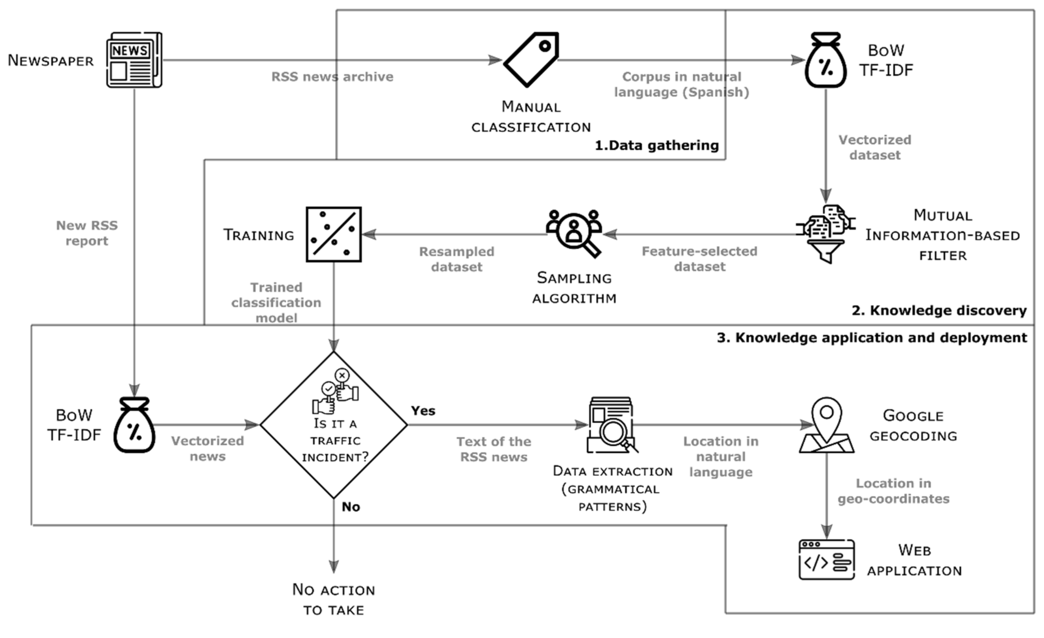
This project is split into three blocks to face the problem of informing citizens about traffic accidents detected automatically in the news reports provided by the RSS service of ‘El Diario de Juárez’ newspaper. These blocks are (a) data gathering, (b) knowledge discovery, and (c) knowledge application and deployment. Figure 2 presents a visual outline of our knowledge-based system, in which the input and output of each process are indicated under the arrows that represent how the data flow, submitting to transformations until becoming into knowledge.

4.1. Data Gathering

‘El Diario de Juárez’ provided an RSS endpoint to which we can remotely connect by using a Python script. Among the data that were provided by the RSS endpoint, the title and the text of news were retrieved. Both fields are in CDATA sections and they have HTML tags embedded and encoded characters, so it was necessary to remove those tags and convert some characters.
Thus, the corpus was generated by a group of volunteer citizens that manually classified the news into twelve classes: crime, public administration, traffic accident, policy, education, health, security, economy, religion, sports, opinion, and others. After manually classifying the news, the corpus consists of 18,386 tagged news, from which 1894 were identified as a traffic accident. Because of the focus of this study, the class was binarized as ‘traffic accident’ and ‘not traffic accident’; therefore, the class of interest became the minority one.

4.2. Knowledge Discovery

In this subsection, Algorithm 1 shows Python-like pseudocode, whose statements are repeatedly referenced by line numbers throughout this subsection to provide a clear picture of how this study can be replicated. For better readability, Algorithm 1 also supplies additional details in the form of comments marked in grey.
The first step in this block is to determine the descriptive vector of each news. For this purpose, we used the BoW technique, which identifies all of the different words from the text of news with their respective occurrences. We utilized the BoW implementation that was provided by the SciKitLearn library [78,79] for the Python language (Lines 1 and 3, where x contains the features and y contains the class). The resultant training dataset has 69,809 integer attributes. Afterward, TF-IDF (term frequency-inverse document frequency) is used to normalize the dataset by calculating the importance of each component (Line 2). Therefore, the words that appear a lot across all news are downscaled.
Algorithm 1 Pseudocode of the knowledge-discovery phase
In: Data: Set of news reports in natural language
  • vector ← vectorizer (Data[Text])       # Data[Text]: News text
  • x ← tfidfTransformer (vector)       # x: Vectorized news text
  • y ← Data[TrafficAccident]    # Data[TrafficAccident]: Binary class of the news
  • fsX ← featureSelector(x, y)    # fsX: x reduced to features selected by the MI filter
  • for each train_index, test_index in KFold (folds = 10)
  • x_train ← fsX[train_index]
  • x_test ← fsX[test_index]
  • y_train ← y[train_index]
  • y_test ← y[test_index]
    • # SMOTE, RndOverSampling, RndUnderSampling, BorderLine SMOTE, AdaSyn
  • smp ← newSamplingAlgorithm ()
  • x_resampled, y_resampled ← smp.fit_resample (x_train, y_train)
    • # SVM, Complement Naïve Bayes, Random Forest, Decision Tree, K-Neighbors
  • classifier ← newClassifierModel ( )
  • classifier.fit (x_resampled, y_resampled)
  • predictions ← classifier.predict (y_test)
  • metrics ← calculateMetrics (y_test, Predictions)
  • print metrics
Before training the classifiers with the vectorized dataset, we reduced its dimensionality to 30,000 features by applying the MI-based filter provided by SciKitLearn (Line 4).
Subsequently, the dataset is split into ten folds to perform cross-validation (Lines 5–9). Afterward, we used sampling algorithms to address the imbalance in the benchmark, because the interest class only represents 10.30% of the instances (Lines 10–11). The sampling algorithms that were tested were SMOTE, borderline SMOTE, ADASYN, ROS, and RUS; all of them taken from the IbmLearn library for the Python language.
After that, we trained the classifiers on the resampled benchmark. The classification algorithms tested were CART, Complement Naïve Bayes, kNN, Random Forest, and SVM (Lines 12–13). We estimated the error rate through 10-fold cross-validation, by whose mean, ranking, and threshold metrics were calculated (Lines 14–16), taking the PR-AUC as the primary measure of discriminatory capacity. The most skillful model is applied in Block 3 to classify. Figure 2 presents the processes of Block 2.

4.3. Knowledge Application and Deployment

When the newspaper issues an RSS news, our application vectorizes it (employing BoW and TF-IDF) and applies the trained SVM model to determine whether it is a traffic accident. For those news reports classified as a traffic accident, a data extraction technique that is based on Spanish grammatical patterns is applied to the text of the news to identify the location of those events. The process follows the next steps:
(a)
sentence segmentation,
(b)
tokenization,
(c)
part of speech tagging (POS),
(d)
named entity recognition (NER), and
(e)
relationship extraction.
All of these steps are performed via SpaCy [80], a Python library. Appendix A offers a more in-depth description of this process with an example.
Once the location has been extracted (in terms of natural language), we used the Google Geocoding API to obtain the coordinates and geolocate them with a marker on a map of the city by using the Google Maps API. Consequently, the content of the map is continuously updated when it detects new information. Anyone can access the application without any cost through a web explorer that is connected to the Internet. Figure 2 also shows the processes performed in Block 3.

5. Results

We programmed our application in Python (version 3.7), using scikit-learn 0.22, imbalanced-learn 0.5, pandas 0.25.3, numpy 1.17.4, matplotlib 3.1.2, SQLAlchemy1.3.15, and MySql 8.0.
Below, we present the experiments conducted to estimate (a) the performance of the classifiers for identifying patterns of the minority class, (b) the improvement through sampling algorithms, and (c) the effectiveness of our approach for extracting locations.

5.1. Performance of the Classifiers on the Imbalanced Corpus

In this experiment, the objective is to identify the most promising classifier to face the case study. Thus, we compared the five supervised learners through performance metrics. The parameter setting for each classifier is the following:
  • CART: criterion = ‘entropy’, and max_depth = None.
  • Complement Naïve Bayes: fit_prior = True, class_prior = None, and norm = False.
  • kNN: n_neighbors = 10, weights = ‘distance’, and p = 2 (euclidian distance).
  • Random Forest: n_estimators = 100, criterion = ‘entropy’, max_depth = None.
  • SVM: loss = ‘hinge’, penalty = ‘l2’, α = 0.001, max_iter = 5, learning_rate = ’optimal’, ε = 0.1, and tol = None.
According to the scientific literature, sensitivity, precision, F1-score, ROC-AUC, and PR-AUC may provide useful information in order to measure the performance of the classifiers on the imbalanced dataset derived from the case study. Table 2 presents, fold by fold, the efficiency of the classifiers in terms of those metrics.
After analyzing averages from Table 2, we may state that:
  • The results from SVM were quite encouraging because this classifier ranked best in terms of PR-AUC (namely the most appropriate measure under conditions of class imbalance), and the second-best in terms of precision, F measure, and ROC-AUC.
  • Random Forest is also remarkable, because it was the best considering ROC-AUC and F1-score, and the second-best in sensitivity and PR-AUC.
  • Although CART obtained the highest recall, it was simultaneously the worst in terms of precision, ROC-AUC, and PR-AUC.
  • Complement Naïve Bayes was only notable in precision, but it was not skillful in recovering instances of the minority class.
  • According to Table 2, kNN (with that setting) seems to be the less fit for classifying this dataset (with the worst values in F-measure and recall).
From this experiment, we identified SVM and Random Forest as the most promising classifiers for this case study. Consequently, we decided to employ sampling algorithms before training in order to enhance the skillfulness of these classifiers.

5.2. Impact of the Sampling Methods on SVM and Random Forest

In this experiment, the objective is to identify the most supportive sampling algorithm for the selected classifiers. The parameter setting for each sampler is the following:
  • SMOTE: sampling_strategy = ‘minority’, k_neighbors = 5, and ratio = None.
  • Borderline SMOTE: sampling_strategy = ‘minority’, k_neighbors = 5, m_neighbors = 10, and kind = ‘borderline-1’.
  • ADASYN: sampling_strategy = ‘minority’, n_neighbors = 5, and ratio = None.
  • ROS: sampling_strategy = ‘minority’, and ratio = None.
  • RUS: sampling_strategy = ‘majority’, replacement = False, and ratio = None.
Table 3 presents the results that were obtained by the two classifiers when enriched with sampling algorithms.
Under this experimental setup and for the case study, we may reach the following conclusions after analyzing Table 3:
  • RUS was the best sampling approach in the scenario where the presence of false negatives is a critical concern (recall).
  • We do not recommend resampling if false positives entail dire consequences (precision).
  • In terms of F1-score, SMOTE and Borderline SMOTE mainly performed well.
  • ROS seems to be the leading choice when considering ROC-AUC alone.
  • Finally, an apparent inconsistency in the impact of sampling methods occurs when PR-AUC is considered decisive. On the one hand, SVM achieved the best results when ROS was applied (followed by RUS). On the other hand, contrary to expectations, no sampling algorithm improved the performance of Random Forest.
For these reasons, we have decided to classify via SVM and resample through ROS. These algorithms jointly offered the best compromise among PR-AUC, ROC-AUC, and sensitivity (it is simultaneously the best one in PR-AUC and ROC-AUC and the third-best in recall). SVM improved its performance by applying ROS prior to training; its metrics were increased in the following manner:
(a)
Recall: from 0.5658 to 0.8558.
(b)
F-measure: from 0.7069 to 0.7828.
(c)
ROC-AUC: from 0.9597 to 0.9693.
(d)
PR-AUC: from 0.8545 to 0.8561.
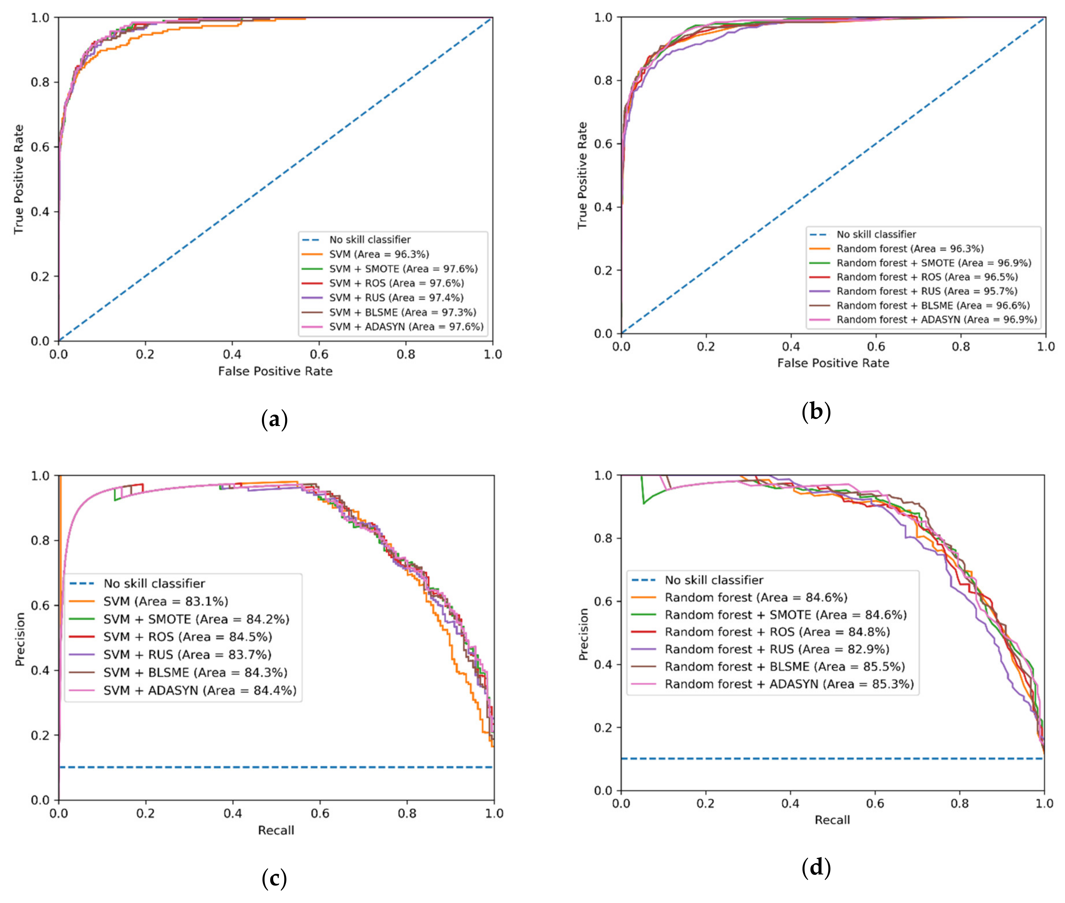
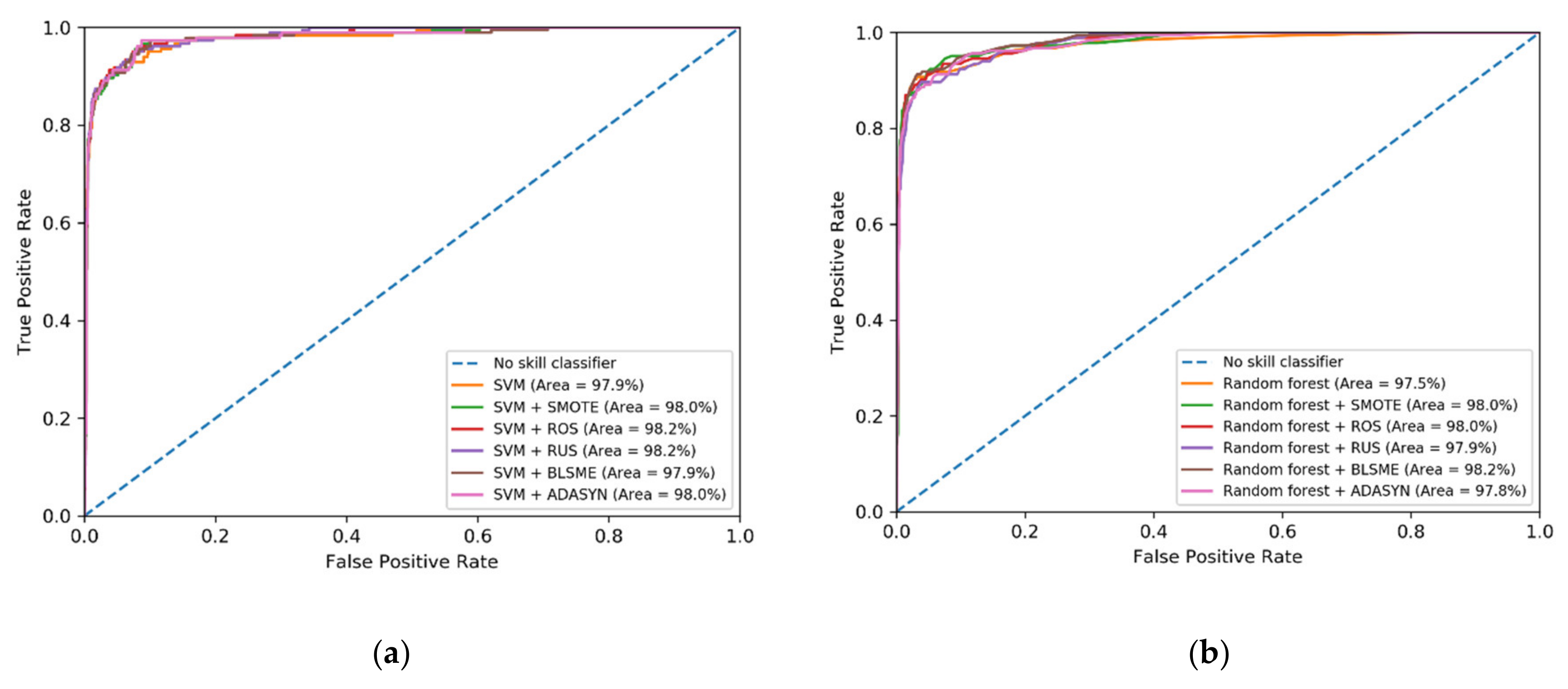
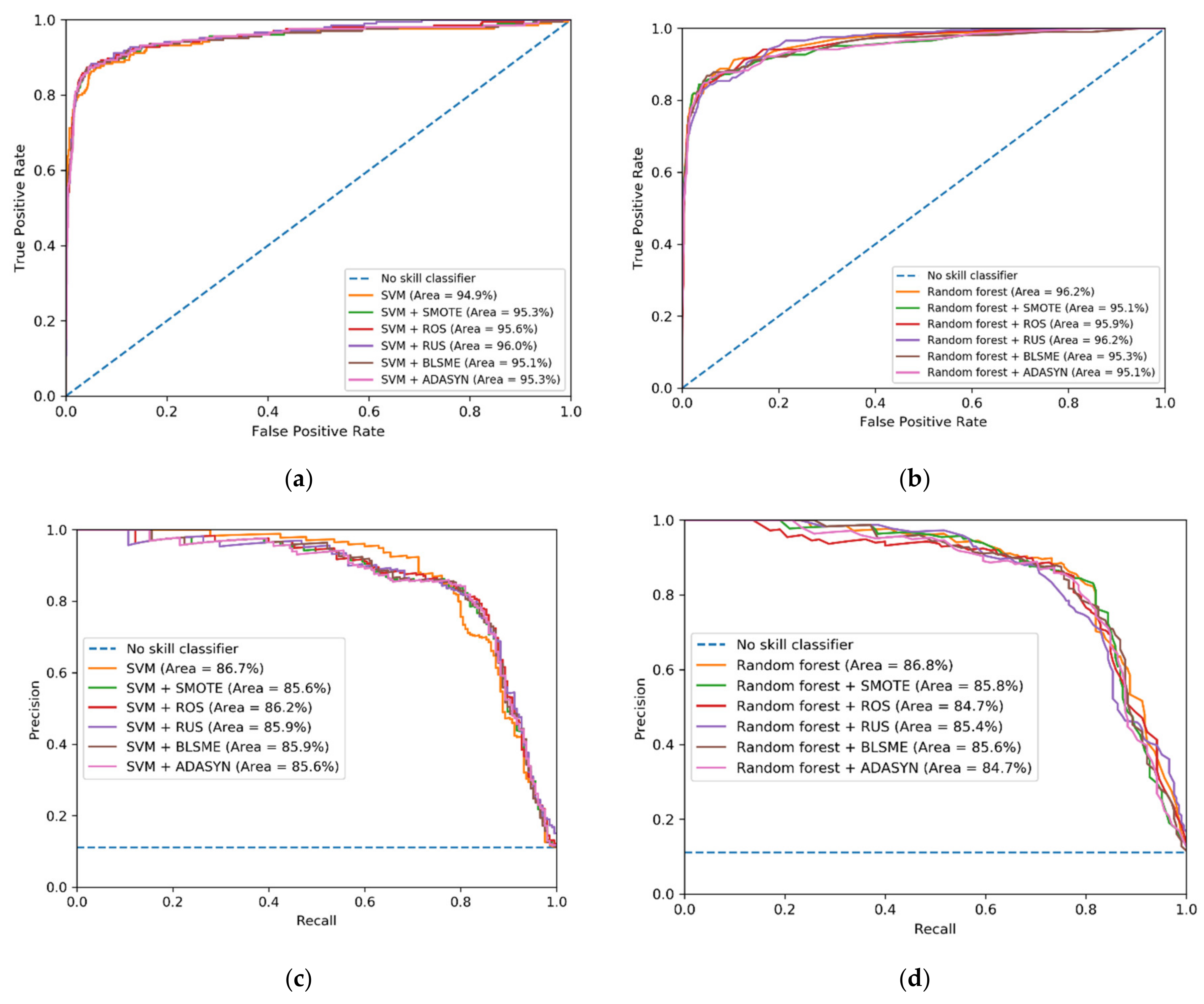
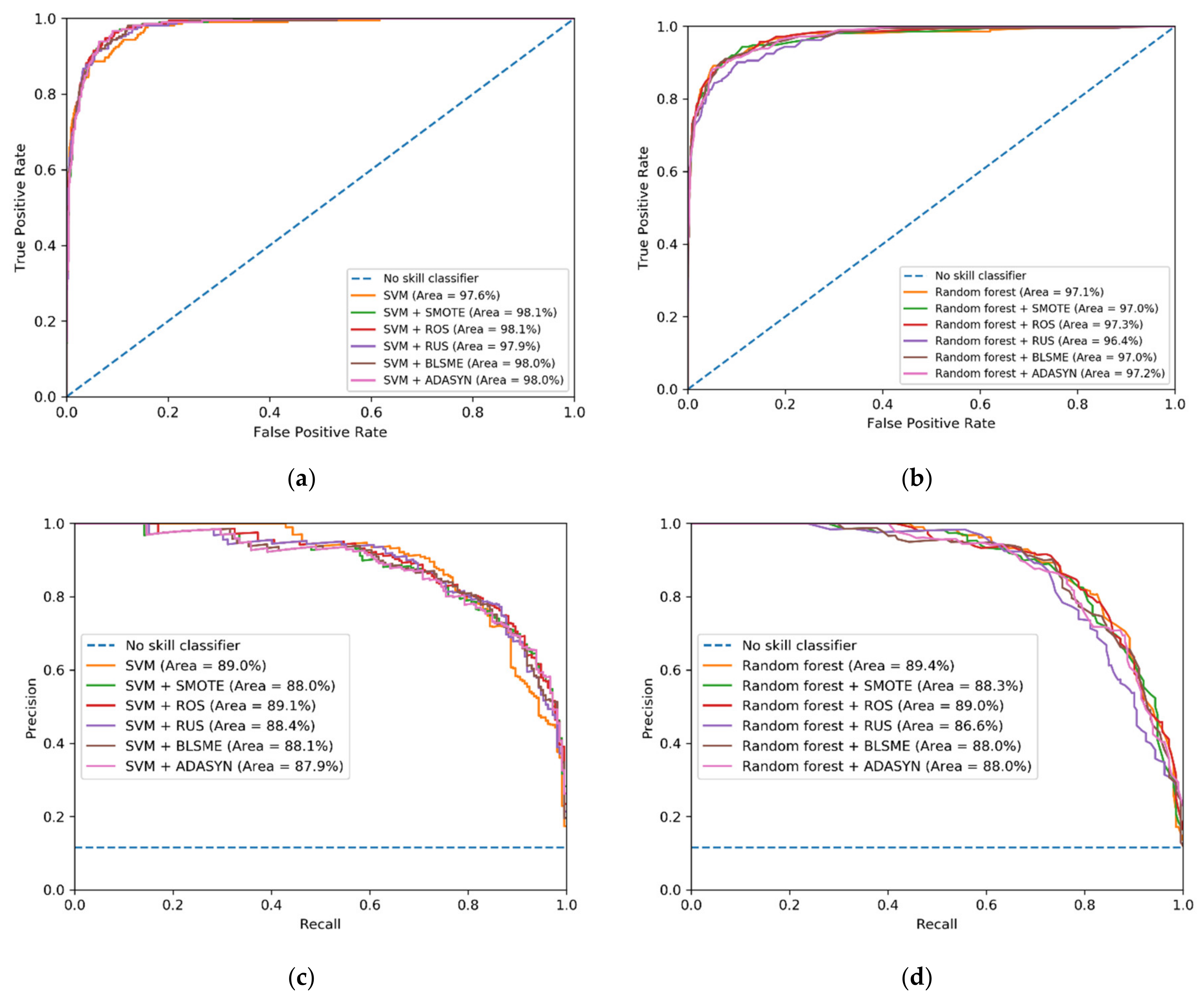
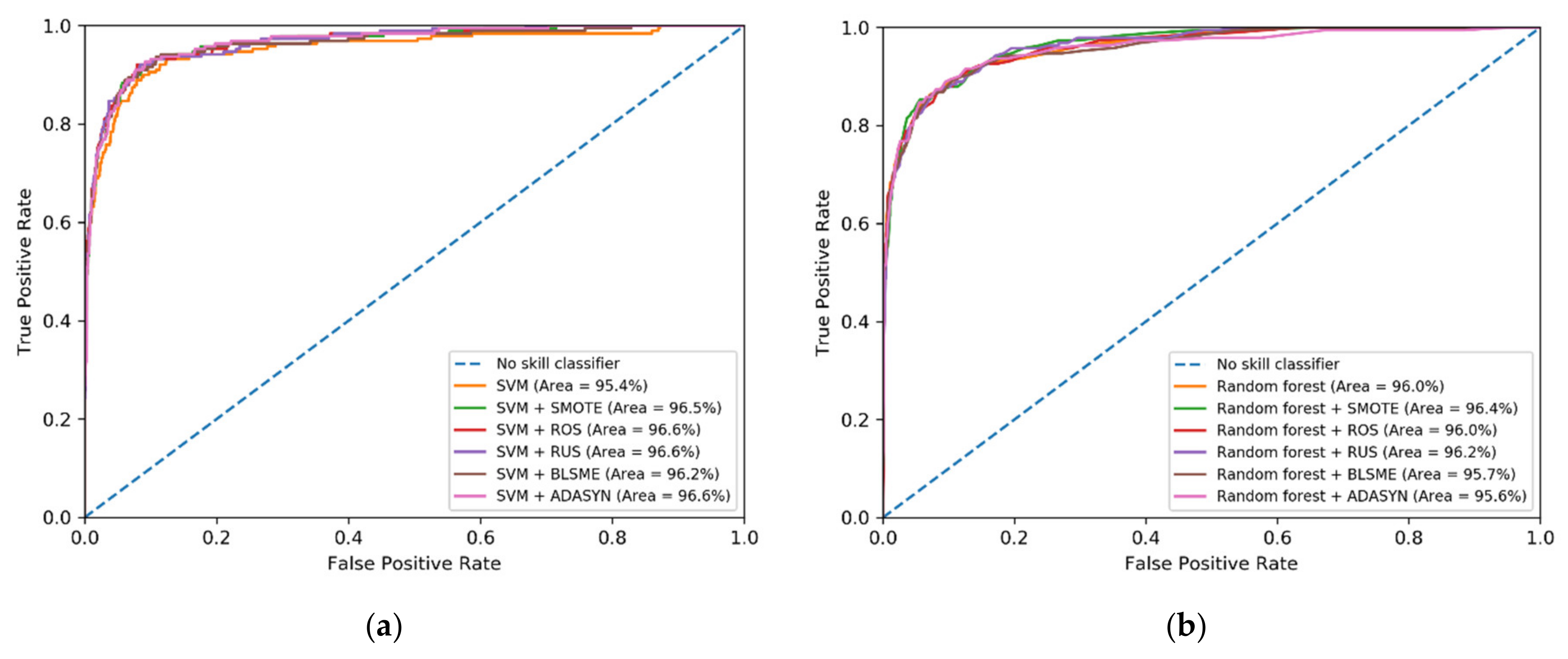
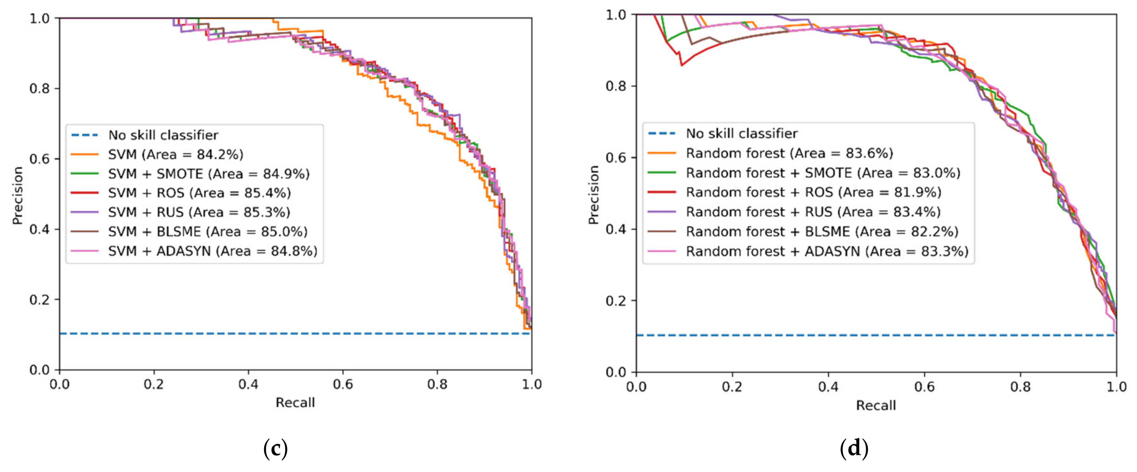
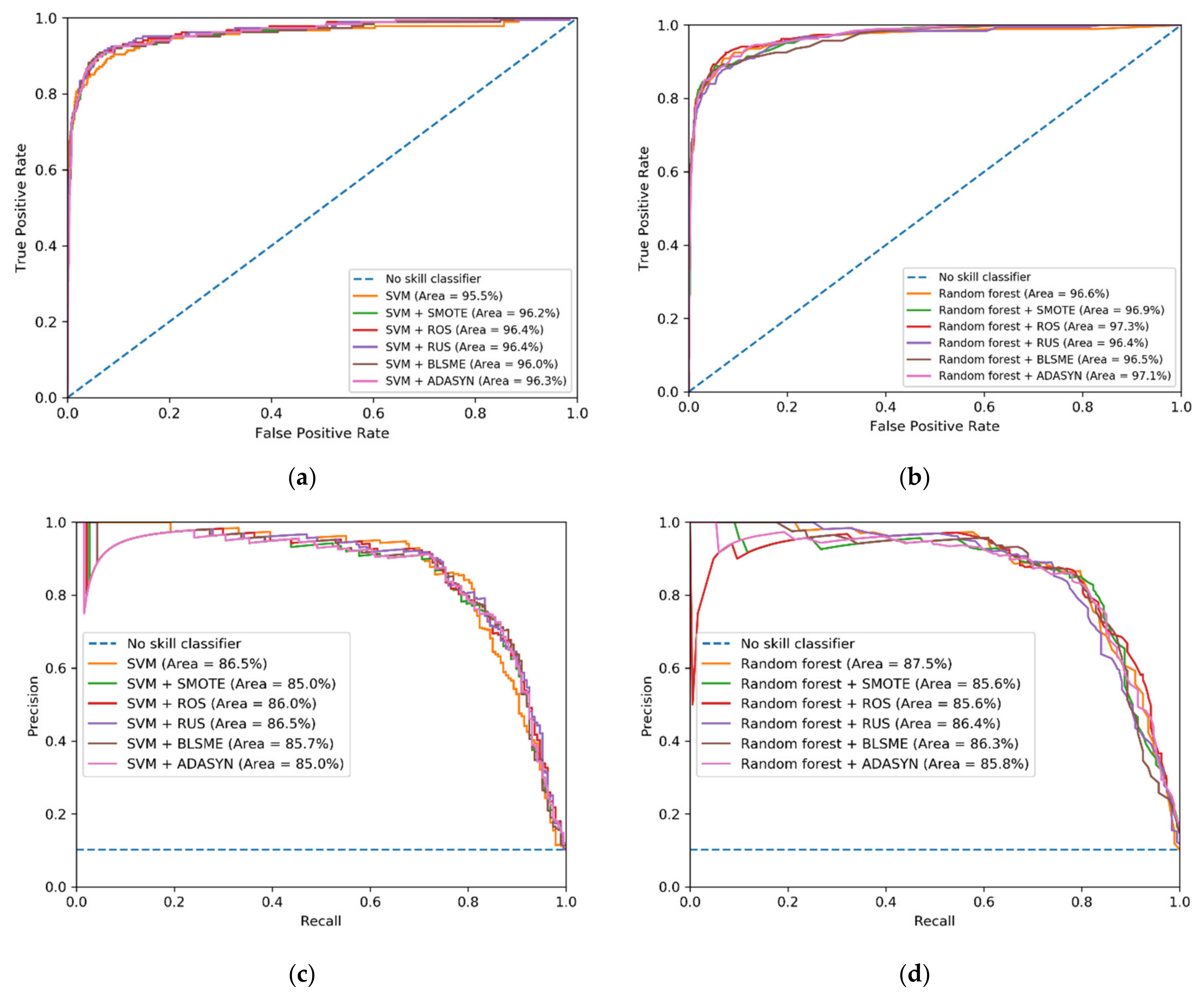
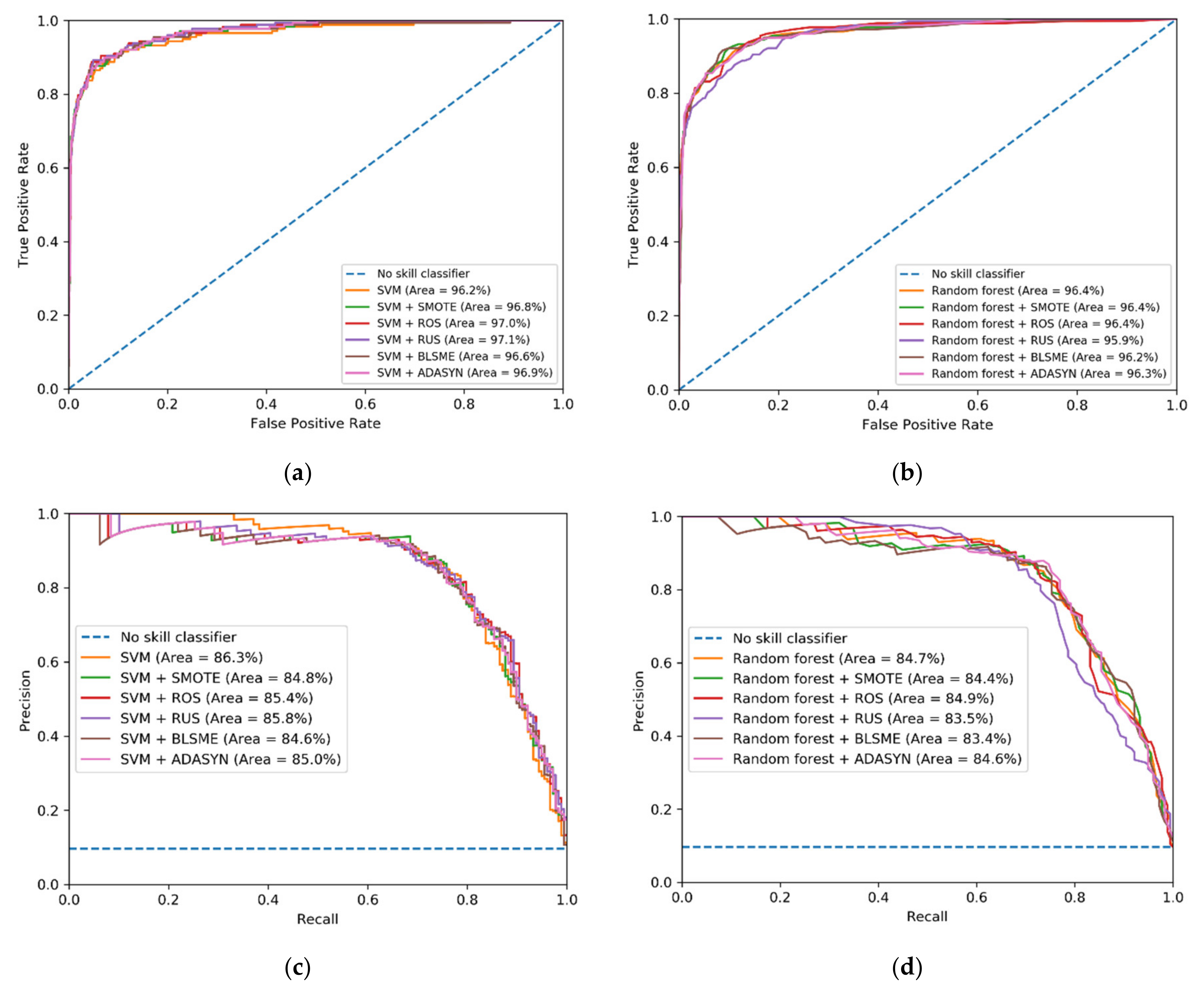
Appendix B contains the plots of the ROC and PR curves, fold-by-fold, for each pair of algorithms in Table 3, which can be checked for further details.

5.3. Performance of the Location Extraction Module

The 2418 new reports the SVM classified as ’traffic accidents’ were used to test the effectiveness of the extractor. Firstly, we carried a filtering process out before presenting the results in the web application. The items that included at least one of the following characteristics were not considered:
  • The report mentioned multiple road mishaps and locations: the data extractor found several fragments of text matching the grammatical rules. However, these locations are not connected to—or close to—a common point when they are geolocated. They often are recapitulations of past news that included traffic accidents.
  • The event occurred outside the city: although the extractor found a fragment of text matching the grammatical patterns, the point is not in the town when it is geolocated.
  • There is not a specified location: the data extractor did not find any match of the grammatical rules.
These filter rules allowed removing 798 RSS news reports (actually, 601 of them are false positives). For the remaining group of 1620 items, the location extractor found matches in all of them; in this sense, it had a 100% rate of success in finding locations in Spanish-written texts. However, let us consider the following two types of result:
(a)
Exact match. There is only a matching fragment of text in which the location was detected, as described in the news exactly.
(b)
Partial matches. The location was detected by several matching fragments of texts.
Partial matches become present when the reports included multiple street names (usually referring to an intersection), or they mentioned a location in a complicated or wordy way. However, we faced this issue when we realized that these partial matching texts often corresponded to the same point when they were geolocated. Subsequently, the location was determined through a majority vote policy.
In the case study, the location extractor offered a performance of 53% of exact matching and 47% of partial matching.

6. Conclusions and Future Work

This paper describes the architecture of a real-world web application whose objective is to identify news reports that are related to traffic incidents, extract their locations, and display them on a map. To this end, it was necessary combinedly applying NLP techniques and machine learning algorithms.
This paper contributes to the literature with a corpus of 18,389 RSS news reports, establishing a standard benchmark for further research on NLP in Spanish. This corpus was made up of news reports from an RSS endpoint provided by the Diario de Juárez, a local newspaper in Mexico, and it is composed of two classes that were manually assigned: ‘traffic accident’ and ‘not traffic accident’. The class of interest is ‘traffic accident’, which is the minority one.
Five classification algorithms were assessed: CART, Complement Naïve Bayes, kNN, Random Forest, and SVM. Before the training process, the corpus was preprocessed by the consecutive application of the bag-of-words technique, TF-IDF normalization, and feature selection based on mutual information. We found SVM and Random Forest as the most skillful classifiers after conducting computational experiments.
By the obtained results, we concluded that the imbalance between both classes negatively affected the performance of both classifiers. Therefore, sampling algorithms were applied to increase their performance in terms of sensitivity and PR-AUC. A comparative analysis was made to select a proper pair of algorithms—classifier and sampler—for addressing this case study. The best results were obtained when random oversampling and SVM were applied together.
In this way, SVM improved the recall 29% (on average) by identifying more patterns belonging to the minority class, without degrading the values of PR-AUC and ROC-AUC (indeed, they were slightly enhanced). This paper empirically evidences the impact of sampling algorithms on the classifiers under conditions of class imbalance and high dimensionality. Random oversampling obtained the most encouraging results among the sampling algorithms tested. Although a side effect of resampling is to diminish precision, NLP techniques based on grammar patterns could mitigate this drawback when they are applied jointly to Machine Learning approaches; in our experiments, the location extraction module was able to identify—indirectly—the 71% of the false-positive cases.
As future work, we are going to explore other ways to represent the RSS news reports. We mean implementing schemata with more capacities than the bag of words, which allow capturing semantic information (e.g., [26,28,29]). Interestingly, the most elementary sampling algorithms—ROS and RUS—proved to be the most effective to address this case study, additional calculations of the other methods did not make any contribution; ergo, we are going to investigate the properties of this corpus (other than its high dimensionality when it is vectorized) to identify the causes and factors behind such behavior; this knowledge would be convenient to face other real-world problems of this nature.

Author Contributions

All authors contributed significantly in writing this paper in the following manner: conceptualization, G.R.; and methodology, R.F. and V.G.; formal analysis, V.G. and P.S.-S; software development, R.F.; writing—original draft preparation, G.R., R.F. and A.R.; writing—review and editing, G.R., R.F. and A.R.; validation, V.G.; data curation, J.P.S-S.; visualization, A.R.; investigation J.P.S.-S. and V.G.; supervision, G.R. All authors have read and agreed to the published version of the manuscript.

Funding

This research received no external funding.

Acknowledgments

The authors gratefully acknowledge the support of the EUREKA Community and the Universidad Autónoma de Ciudad Juárez (División Multidisciplinaria de Ciudad Universitaria).

Conflicts of Interest

The authors declare no conflict of interest.

Appendix A

Here, a technique of information extraction is applied to all the news that we have classified as a traffic accident, which is the input set to extract the location from the news text.
We used a library for NLP called spaCy [80] for the extraction module, which employs a rule-based matching. This process works by defining a set of rules composed by elements like punctuation marks, the length of a token, tokens in uppercase or lowercase, grammatical tags, among others. Once the rules are defined, they are applied to a news report; if there are one or more matches, the location is obtained from the text. The group of rules for the location extraction was created by considering the grammatical structure with which the point of a traffic accident can be written. The rules that form the description of roadways are the following:
(a)
A prefix to indicate the kind of road (either in singular or plural) followed by an optional article and preposition (e.g., ‘carretera de’, ‘avenida de la’, ‘Bulevar’, ‘periférico’).
(b)
The name of the road with an elective number followed by as far as four words in a little case format with an optional grammatical article and preposition between each one of them (e.g., ‘calle Norte’, ‘periférico de la Juventud’, ‘bulevar Juan Pablo II’, ‘calle 20 de noviembre’).
This set of rules can be repeated one time with a conjunction between them; forming the pattern used in this extraction module.
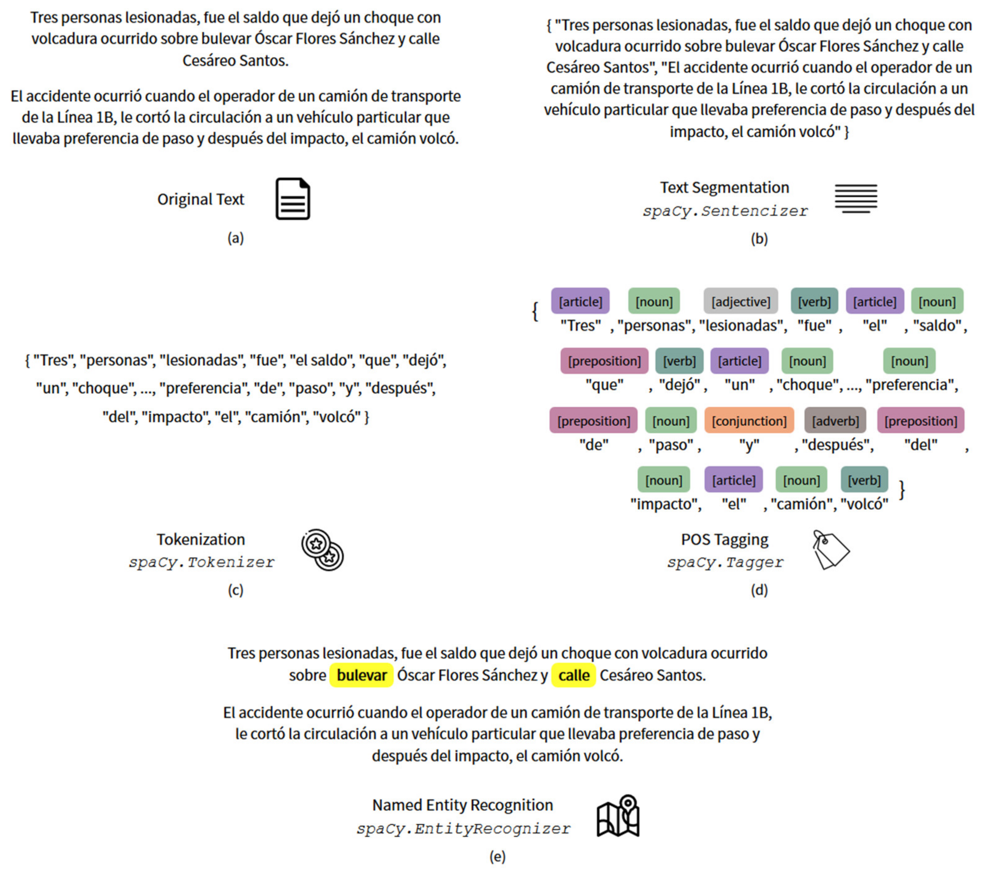
Figure A1 presents an example of how the extraction module works over a news report. In Figure A1a, the content of a news report is the input, obtained after preprocessing the element got from the RSS endpoint, which is only plain text in Spanish. In Figure A1b, the original text is divided into its composing sentences through the Sentencizer class, which will mainly split the original text by period; although other symbols may mark the end of a sentence, those are less common in the text of a news report. In Figure A1c, the Tokenizer class takes the set of sentences obtained previously and breaks down the text into its most basic units (tokens). In Figure A1d, the POS tagging process is benefited by the tokenization step; the Tagger class takes each one of the tokens and assigns its grammatical function. Finally, in Figure A1e performs the Named Entity Recognition through the EntityRecognizer class to identify the entities we are interested in that could help to find the location. Since we are only interested in entities referring to a roadway (in Spanish, this list includes ‘calle’, ‘avenida’, ‘bulevar’, ‘carretera’, among others), this step identifies ‘bulevar’ and ‘calle’ as the meaningful words.
Once all of these steps are done, the Matcher class tries to find sequences of tokens that match the pattern rules. In this case, the extraction is exact and performs a single match that identifies an intersection formed by two roadways: ‘bulevar Óscar Flores Sánches y calle Cesáreo Santos’. Because no additional steps are needed, this is stored in a database as the extracted location.
Figure A1. Processing for the Information Extraction process: (a) Original Text; (b) Text Segmentation; (c) Tokenization; (d) POS Tagging; and, (e) Named Entity Recognition.
Applsci 10 06253 g0a1

Appendix B

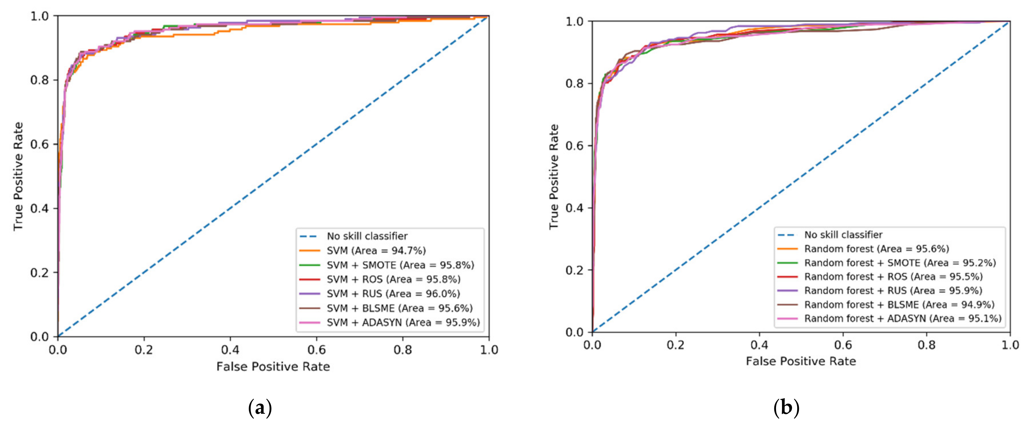
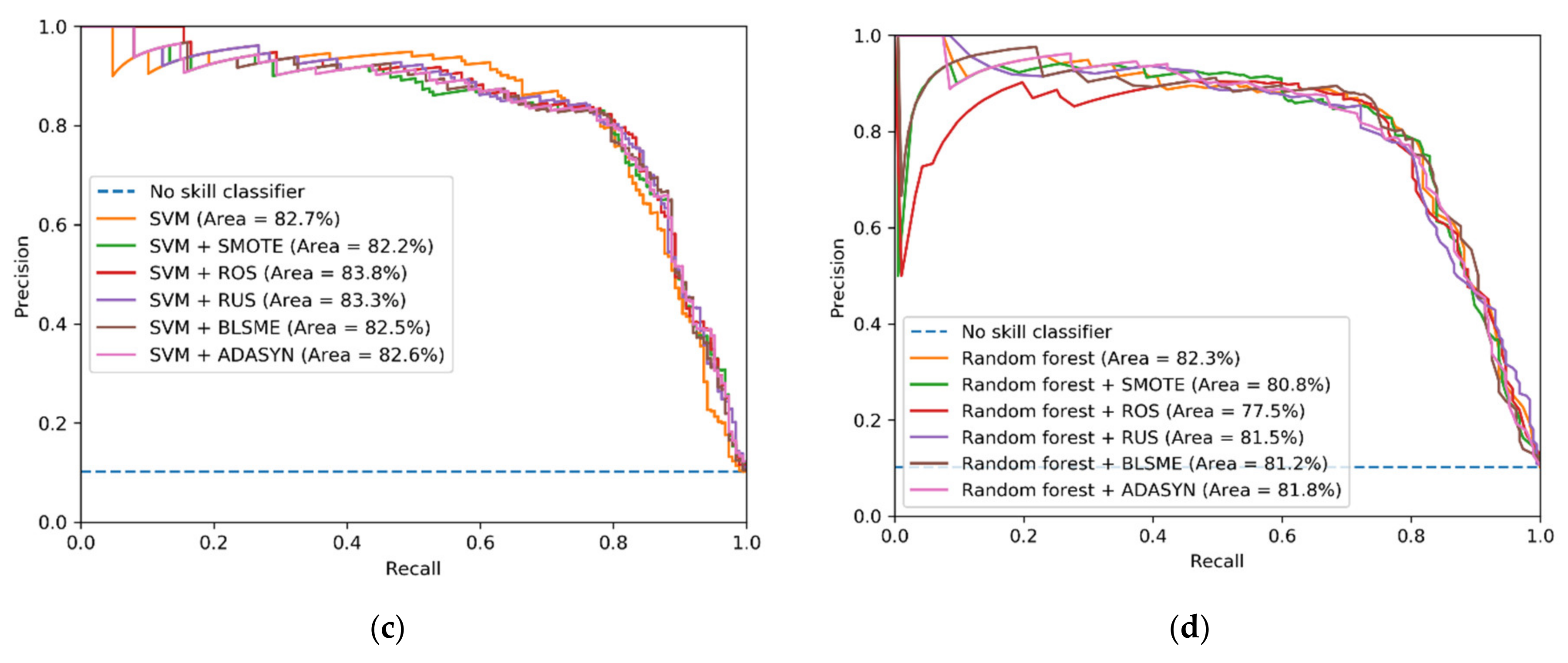
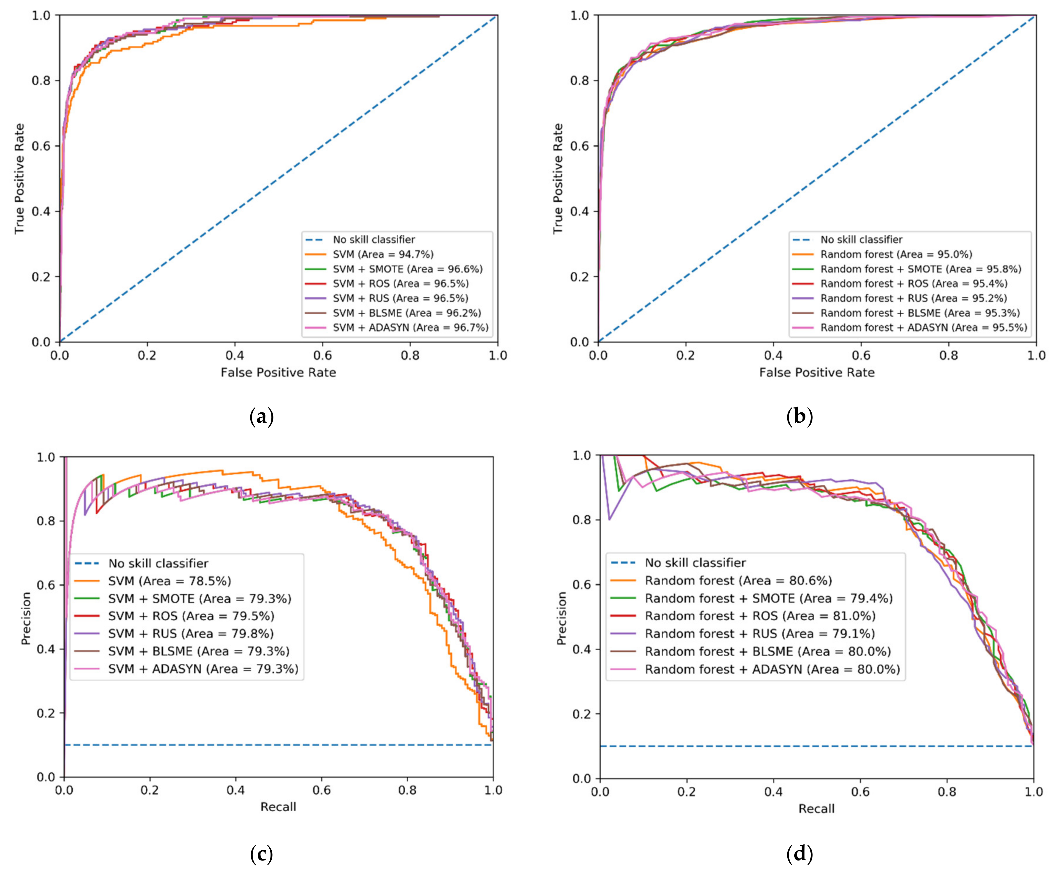
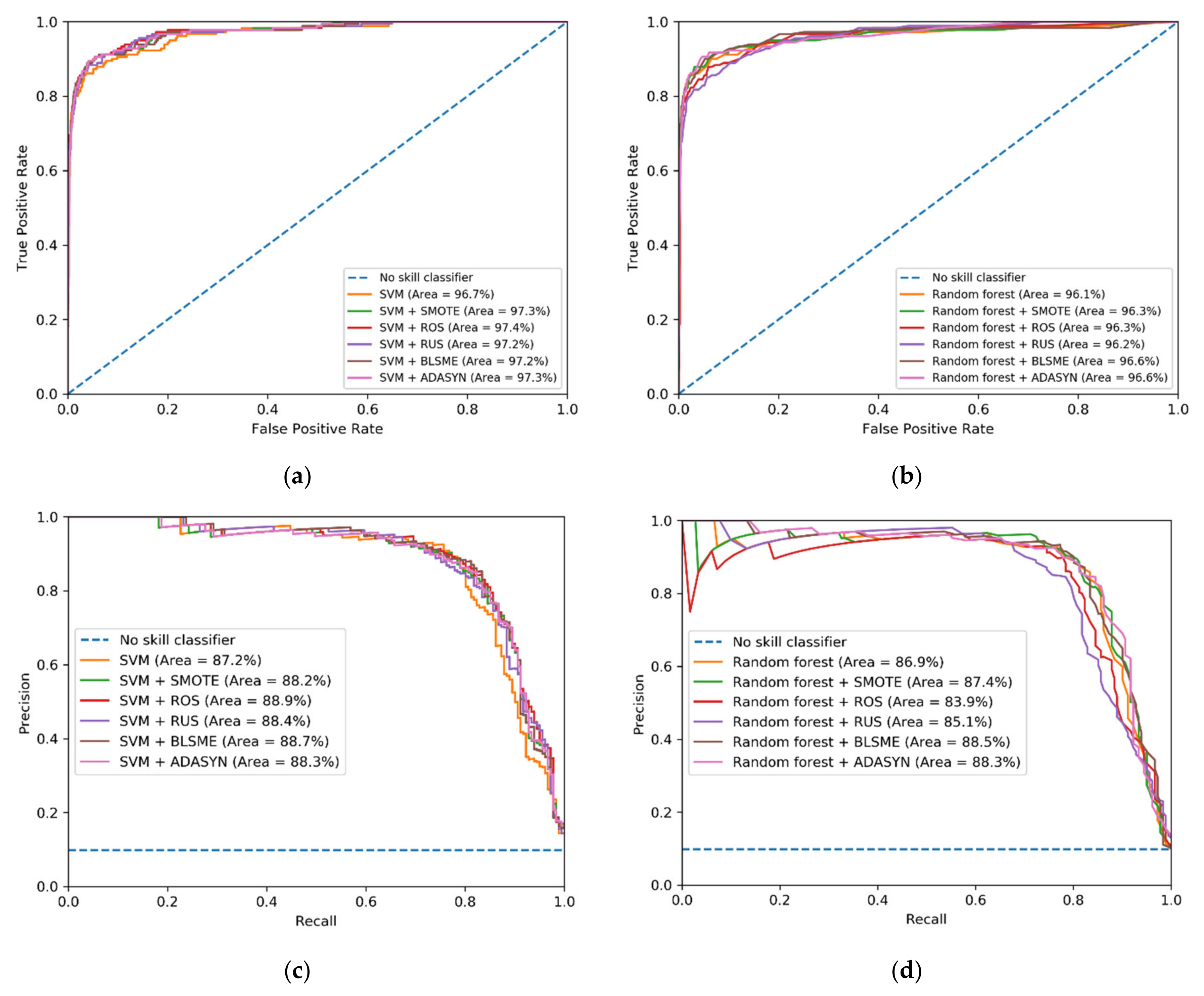
This appendix presents, in Figure A2, Figure A3, Figure A4, Figure A5, Figure A6, Figure A7, Figure A8, Figure A9, Figure A10 and Figure A11, the ROC and PR curves of SVM and Random Forest, fold by fold, incorporating sampling algorithms.
Figure A2. The ROC and PR curves of SVM and Random Forest for Fold 1; (a) the ROC curve of SVM; (b) the ROC curve of Random Forest; (c) the PR curve of SVM; and, (d) the PR curve of Random Forest.
Applsci 10 06253 g0a2
Figure A3. The ROC and PR curves of SVM and Random Forest for Fold 2; (a) the ROC curve of SVM; (b) the ROC curve of Random Forest; (c) the PR curve of SVM; and, (d) the PR curve of Random Forest.
Applsci 10 06253 g0a3aApplsci 10 06253 g0a3b
Figure A4. The ROC and PR curves of SVM and Random Forest for Fold 3; (a) the ROC curve of SVM; (b) the ROC curve of Random Forest; (c) the PR curve of SVM; and, (d) the PR curve of Random Forest.
Applsci 10 06253 g0a4
Figure A5. The ROC and PR curves of SVM and Random Forest for Fold 4; (a) the ROC curve of SVM; (b) the ROC curve of Random Forest; (c) the PR curve of SVM; and, (d) the PR curve of Random Forest.
Applsci 10 06253 g0a5
Figure A6. The ROC and PR curves of SVM and Random Forest for Fold 5; (a) the ROC curve of SVM; (b) the ROC curve of Random Forest; (c) the PR curve of SVM; and, (d) the PR curve of Random Forest.
Applsci 10 06253 g0a6aApplsci 10 06253 g0a6b
Figure A7. The ROC and PR curves of SVM and Random Forest for Fold 6; (a) the ROC curve of SVM; (b) the ROC curve of Random Forest; (c) the PR curve of SVM; and, (d) the PR curve of Random Forest.
Applsci 10 06253 g0a7
Figure A8. The ROC and PR curves of SVM and Random Forest for Fold 7; (a) the ROC curve of SVM; (b) the ROC curve of Random Forest; (c) the PR curve of SVM; and, (d) the PR curve of Random Forest.
Applsci 10 06253 g0a8
Figure A9. The ROC and PR curves of SVM and Random Forest for Fold 8; (a) the ROC curve of SVM; (b) the ROC curve of Random Forest; (c) the PR curve of SVM; and, (d) the PR curve of Random Forest.
Applsci 10 06253 g0a9aApplsci 10 06253 g0a9b
Figure A10. The ROC and PR curves of SVM and Random Forest for Fold 9; (a) the ROC curve of SVM; (b) the ROC curve of Random Forest; (c) the PR curve of SVM; and, (d) the PR curve of Random Forest.
Applsci 10 06253 g0a10
Figure A11. The ROC and PR curves of SVM and Random Forest for Fold 10; (a) the ROC curve of SVM; (b) the ROC curve of Random Forest; (c) the PR curve of SVM; and, (d) the PR curve of Random Forest.
Applsci 10 06253 g0a11

References

  1. United Nations. World Urbanization Prospects 2018. Available online: https://population.un.org/wup/ (accessed on 1 September 2020).
  2. United Nations. World’s Population Increasingly Urban with More than Half Living in Urban Areas. Available online: http://un.org/en/development/desa/news/population/world-urbanization-prospects-2014.html (accessed on 1 September 2020).
  3. Ochoa Ortiz-Zezzatti, A.; Rivera, G.; Gómez-Santillán, C.; Sánchez-Lara, B. Handbook of Research on Metaheuristics for Order Picking Optimization in Warehouses to Smart Cities; IGI Global: Hershey, PA, USA, 2019. [Google Scholar] [CrossRef]
  4. Smart Cities Council. Smart Cities A to Z. Glossary, letter “S”. Available online: http://rg.smartcitiescouncil.com/master-glossary/S (accessed on 1 September 2020).
  5. Williams, P. What, Exactly, is a Smart City? Available online: http://meetingoftheminds.org/exactly-smart-city-16098 (accessed on 1 September 2020).
  6. Harris, Z.S. Distributional structure. Word 1954, 10, 146–162. [Google Scholar] [CrossRef]
  7. Kaur, H.; Pannu, H.S.; Malhi, A.K. A systematic review on imbalanced data challenges in machine learning: Applications and solutions. CSUR 2019, 52, 1–36. [Google Scholar] [CrossRef] [Green Version]
  8. Zhang, C.; Bi, J.; Xu, S.; Ramentol, E.; Fan, G.; Qiao, B.; Fujita, H. Multi-imbalance: An open-source software for multi-class imbalance learning. Knowl. Based Syst. 2019, 174, 137–143. [Google Scholar] [CrossRef]
  9. Krawczyk, B. Learning from imbalanced data: Open challenges and future directions. Prog. Artif. Intell. 2016, 5, 221–232. [Google Scholar] [CrossRef] [Green Version]
  10. Fernández, A.; García, S.; Herrera, F. Addressing the classification with imbalanced data: Open problems and new challenges on class distribution. In International Conference on Hybrid Artificial Intelligence Systems; Springer: Berlin/Heidelberg, Germany, 2011; pp. 1–10. [Google Scholar]
  11. Lane, J. The 10 Most Spoken Languages in The World. Available online: http://babbel.com/en/magazine/the-10-most-spoken-languages-in-the-world (accessed on 1 September 2020).
  12. Internet World Stats. Internet World Users by Language: Top 10 Languages. Usage and Population Statistics. Available online: https://www.internetworldstats.com/stats7.htm (accessed on 1 September 2020).
  13. Aliwy, A.H.; Ameer, E.A. Comparative study of five text classification algorithms with their improvements. Int. J. Appl. Eng. Res. 2017, 12, 4309–4319. [Google Scholar]
  14. Allahyari, M.; Pouriyeh, S.; Assefi, M.; Safaei, S.; Trippe, E.D.; Gutierrez, J.B.; Kochut, K. A Brief Survey of Text Mining: Classification, Clustering and Extraction Techniques. arXiv, 2017; arXiv:1707.02919. [Google Scholar]
  15. Thangaraj, M.; Sivakami, M. Text Classification Techniques: A Literature Review. Interdiscip. J. Inf. Knowl. Manag. 2018, 13, 117–135. [Google Scholar]
  16. Steinberg, D.; Colla, P. CART: Classification and Regression Trees. Top Ten Algorithms Data Min. 2009, 9, 179–201. [Google Scholar]
  17. Cutler, A.; Cutler, D.R.; Stevens, J.R. Random forests. In Ensemble Machine Learning; Springer: Boston, MA, USA, 2012; pp. 157–175. [Google Scholar]
  18. Berrar, D. Bayes’ theorem and naïve Bayes classifier. In Encyclopedia of Bioinformatics and Computational Biology: ABC of Bioinformatics; Elsevier Science Publisher: Amsterdam, The Netherlands, 2018; pp. 403–412. [Google Scholar]
  19. Catal, C.; Nangit, M. A sentiment classification model based on multiple classifiers. Appl. Soft Comput. 2017, 50, 135–141. [Google Scholar] [CrossRef]
  20. Ghaddar, B.; Naoum-Sawaya, J. High dimensional data classification and feature selection using support vector machines. Eur. J. Oper. Res. 2018, 265, 993–1004. [Google Scholar] [CrossRef]
  21. Goudjil, M.; Koudil, M.; Bedda, M.; Ghoggali, N. A novel active learning method using SVM for text classification. Int. J. Autom. Comput. 2018, 15, 290–298. [Google Scholar] [CrossRef]
  22. Hu, R.; Namee, B.M.; Delany, S.J. Active learning for text classification with reusability. Expert Syst. Appl. 2016, 45, 438–449. [Google Scholar] [CrossRef]
  23. Lilleberg, J.; Zhu, Y.; Zhang, Y. Support Vector Machines and word2vec for Text Classification with Semantic Features. In Proceedings of the 14th IEEE International Conference on Cognitive Informatics and Cognitive Computing, Beijing, China, 6–8 July 2015; pp. 136–140. [Google Scholar]
  24. Onan, A.; Korukoğlu, S.; Bulut, H. Ensemble of keyword extraction methods and classifiers in text classification. Expert Syst. Appl. 2016, 57, 232–247. [Google Scholar] [CrossRef]
  25. Xia, H.; Yang, Y.; Pan, X.; Zhang, Z.; An, W. Sentiment analysis for online reviews using conditional random fields and support vector machines. Electron. Commer. Res. 2020, 20, 343–360. [Google Scholar] [CrossRef]
  26. El-Din, D.M. Enhancement bag-of-words model for solving the challenges of sentiment analysis. Int. J. Adv. Comput. Sci. Appl. 2016, 7. [Google Scholar] [CrossRef] [Green Version]
  27. Fu, Y.; Feng, Y.; Cunningham, J.P. Paraphrase Generation with Latent Bag of Words. In Advances in Neural Information Processing Systems; MIT Press: Vancouver, BC, Canada, 2019; pp. 13623–13634. [Google Scholar]
  28. Kim, H.K.K.H.; Cho, S. Bag-of-concepts: Comprehending document representation through clustering words in distributed representation. Neurocomputing 2017, 266, 336–352. [Google Scholar] [CrossRef] [Green Version]
  29. Zhao, R.; Mao, K. Fuzzy bag-of-words model for document representation. IEEE Trans. Fuzzy Syst. 2017, 26, 794–804. [Google Scholar] [CrossRef]
  30. Aggarwal, C.C.; Zhai, C. A Survey of Text Classification Algorithms. In Mining Text Data; Springer: Berlin/Heidelberg, Germany, 2012; pp. 163–222. [Google Scholar]
  31. Vergara, J.R.; Estévez, P.A. A review feature selection methods based on mutual information. Neural. Comput. Appl. 2014, 24, 175–186. [Google Scholar] [CrossRef]
  32. Haixiang, G.; Yijing, L.; Shang, J.; Mingyun, G.; Yuanyue, H.; Bing, G. Learning from class-imbalanced data: Review of methods and applications. Expert Syst. Appl. 2017, 73, 220–239. [Google Scholar] [CrossRef]
  33. García, V.; Sánchez, J.S.; Marqués, A.I.; Florencia, R.; Rivera, G. Understanding the apparent superiority of over-sampling through an analysis of local information for class-imbalanced data. Expert Syst. Appl. 2019, 113026. [Google Scholar] [CrossRef]
  34. Chawla, N.V.; Bowyer, K.W.; Hall, L.O.; Kegelmeyer, W.P. SMOTE: Synthetic Minority Over-Sampling Technique. J. Artif. Intell. Res. 2002, 16, 321–357. [Google Scholar] [CrossRef]
  35. Han, H.; Wang, W.Y.; Mao, B.H. Borderline-SMOTE: A new over-sampling method in imbalanced data sets learning. In International Conference on Intelligent Computing; Springer: Berlin/Heidelberg, Germany, 2005; pp. 878–887. [Google Scholar]
  36. He, H.; Bai, Y.; Garcia, E.A.; Li, S. ADASYN: Adaptive Synthetic Sampling Approach for Imbalanced Learning. In Proceedings of the 2008 IEEE International Joint Conference on Neural Networks, Hong Kong, China, 1–8 June 2008; pp. 1322–1328. [Google Scholar]
  37. Fernández, A.; García, S.; Galar, M.; Prati, R.C.; Krawczyk, B.; Herrera, F. Learning from Imbalanced Data Sets; Springer: Berlin/Heidelberg, Germany, 2018; pp. 1–377. [Google Scholar]
  38. He, H.; Ma, Y. Imbalanced Learning: Foundations, Algorithms, and Applications; John Wiley & Sons: Hoboken, NJ, USA, 2013. [Google Scholar]
  39. Branco, P.; Torgo, L.; Ribeiro, R.P. A survey of predictive modeling on imbalanced domains. CSUR 2016, 49, 1–150. [Google Scholar] [CrossRef]
  40. Luhn, H.P. A statistical approach to mechanized encoding and searching of literary information. IBM J. Res. Dev. 1957, 1, 309–317. [Google Scholar] [CrossRef]
  41. Maron, M.E.; Kuhns, J.L. On relevance, probabilistic indexing and information retrieval. JACM 1960, 7, 216–244. [Google Scholar] [CrossRef]
  42. Arthur Frederick Parker-Rhodes. Contributions to the Theory of Clumps I; Cambridge Language Research Unit: Cambridge, UK, 1961; pp. 1–27. [Google Scholar]
  43. Sebastiani, F. Machine learning in automated text categorization. CSUR 2002, 34, 1–47. [Google Scholar] [CrossRef]
  44. Joachims, T. Text categorization with support vector machines: Learning with many relevant features. In European Conference Machine Learning; Springer: Berlin/Heidelberg, Germany, 1998; pp. 137–142. [Google Scholar]
  45. Zhuang, D.; Zhang, B.; Yang, Q.; Yan, J.; Chen, Z.; Chen, Y. Efficient text classification by weighted proximal SVM. In Proceedings of the Fifth IEEE International Conference on Data Mining, Houston, TX, USA, 27–30 November 2005; p. 8. [Google Scholar]
  46. Liu, Z.; Lv, X.; Liu, K.; Shi, S. Study on SVM compared with the other classification methods. In Proceedings of the 2010 Second International Workshop Education Technology and Computer Science, Wuhan, China, 6–7 March 2010; IEEE: Piscataway, NJ, USA, 2010; Volume 1, pp. 219–222. [Google Scholar]
  47. Kumar, M.A.; Gopal, M. An Investigation on Linear SVM and its Variants on Text Categorization. In Proceedings of the 2010 Second International Conference Machine Learning and Computing, Bangalore, India, 12–13 February 2010; IEEE: Piscataway, NJ, USA, 2010; pp. 27–31. [Google Scholar]
  48. Friedman, N.; Geiger, D.; Goldszmidt, M. Bayesian network classifiers. Mach. Learn. 1997, 29, 131–163. [Google Scholar] [CrossRef] [Green Version]
  49. Boyle, J.A.; Greig, W.R.; Franklin, D.A.; Harden, R.M.; Buchanan, W.W.; McGirr, E.M. Construction of a model for computer assisted diagnosis: Application of the problem of non-toxic goitre. QJM 1966, 35, 565–588. [Google Scholar]
  50. Penny, W.D.; Frost, D.P. Neural network modeling of the level of observation decision in an acute psychiatric ward. Comput. Biomed. Res. 1997, 30, 1–17. [Google Scholar] [CrossRef]
  51. Xu, S. Naïve Bayes classifiers to text classification. J. Inf. Sci. 2018, 44, 48–59. [Google Scholar] [CrossRef]
  52. Friedman, J.H. On bias, variance, 0/1–loss, and the curse-of-dimensionality. Data Min. Knowl. Discov. 1997, 1, 55–77. [Google Scholar] [CrossRef]
  53. McCallum, A.; Nigam, K. A comparison of event models for naïve Bayes text classification. In AAAI-98 Workshop on Learning for Text Categorization; AAAI Press: Madison, WI, USA, 27 July 1998; Volume 752, pp. 41–48. [Google Scholar]
  54. Xu, B.; Guo, X.; Ye, Y.; Cheng, J. An Improved Random Forest Classifier for Text Categorization. JCP 2012, 7, 2913–2920. [Google Scholar] [CrossRef] [Green Version]
  55. Tan, S. Neighbor-weighted k-nearest neighbor for unbalanced text corpus. Expert Syst. Appl. 2005, 28, 667–671. [Google Scholar] [CrossRef] [Green Version]
  56. Yong, Z.; Youwen, L.; Shixiong, X. An improved KNN text classification algorithm based on clustering. J. Comput. 2009, 4, 230–237. [Google Scholar]
  57. Sriram, B.; Fuhry, D.; Demir, E.; Ferhatosmanoglu, H.; Demirbas, M. Short text classification in twitter to improve information filtering. In Proceedings of the 33rd ACM SIGIR International Conference of Research and Development on Information Retrieval, Geneva, Switzerland, 19–23 July 2010; pp. 841–842. [Google Scholar]
  58. Burnap, P.; Williams, M.L. Cyber hate speech on twitter: An application of machine classification and statistical modeling for policy and decision making. Policy Internet. 2015, 7, 223–242. [Google Scholar] [CrossRef] [Green Version]
  59. Dilrukshi, I.; de Zoysa, K.; Caldera, A. Twitter news classification using SVM. In Proceedings of the 8th International Conference on Computer Science & Education, Colombo, Sri Lanka, 26–28 April 2013; pp. 287–291. [Google Scholar]
  60. Song, G.; Ye, Y.; Du, X.; Huang, X.; Bie, S. Short text classification: A survey. J. Multimed. 2014, 9, 635. [Google Scholar] [CrossRef]
  61. Hofmann, T. Probabilistic Latent Semantic Analysis. arXiv, 1999; arXiv:1301.6705. [Google Scholar]
  62. L’Huillier, G.; Hevia, A.; Weber, R.; Rios, S. Latent semantic análisis and keyword extraction for phishing classification. In Proceedings of the 2010 IEEE International Conference on Intelligence and Security Informatics, Vancouver, BC, Canada, 23–26 May 2010; pp. 129–131. [Google Scholar]
  63. Zeng, Z.; Zhang, S.; Liang, H.L.W.; Zheng, H. A novel approach to musical genre classification using probabilistic latent semantic analysis model. In Proceedings of the 2009 IEEE International Conference on Multimedia and Expo, Cancun, Mexico, 28 June–3 July 2009; pp. 486–489. [Google Scholar]
  64. Bosch, A.; Zisserman, A.; Muñoz, X. Scene classification via pLSA. In European Conference Computer Vision; Springer: Berlin/Heidelberg, Germany, 2006; pp. 517–530. [Google Scholar]
  65. Díaz, G.; Romero, E. Histopathological Image Classification Using Stain Component Features on a pLSA Model. In Iberoamerican Congress Pattern Recognition; Springer: Berlin/Heidelberg, Germany, 2010; pp. 55–62. [Google Scholar]
  66. Haloi, M. A novel pLSA based Trafic Signs Classification System. arXiv, 2015; arXiv:abs/1503.06643. [Google Scholar]
  67. Kroha, P.; Baeza-Yates, R. A Case Study: News Classification Based on Term Frequency. In Proceedings of the 16th International Workshop on Database and Expert Systems Applications, Copenhagen, Denmark, 22–26 August 2005; pp. 428–432. [Google Scholar]
  68. Mouriño-García, M.A.; Pérez-Rodríguez, R.; Anido-Rifón, L.; Vilares-Ferro, M. Wikipedia-based hybrid document representation for textual news classification. Soft Comput. 2018, 22, 6047–6065. [Google Scholar] [CrossRef]
  69. Sankaranarayanan, J.; Samet, H.; Teitler, B.E.; Lieberman, M.D.; Sperling, J. Twitterstand: News in Tweets. In Proceedings of the 17th ACM SIGSPATIAL International Conference on Advances in Geographic Information Systems, Seattle, WA, USA, 4–6 November 2009; pp. 42–51. [Google Scholar]
  70. Li, C.; Zhan, G.; Li, Z. News text classification based on improved Bi-LSTM-CNN. In Proceedings of the IEEE 9th International Conference on Information Technology in Medicine and Education, Hangzhou, China, 19–21 October 2018; pp. 890–893. [Google Scholar]
  71. Dadgar, S.M.H.; Araghi, M.S.; Farahani, M.M. A novel text mining approach based on TF-IDF and Support Vector Machine for news classification. In Proceedings of the 2016 IEEE Internatoonal Conference Engineering and Technology, Coimbatore, India, 17–18 March 2016; pp. 112–116. [Google Scholar]
  72. Bondielli, A.; Marcelloni, F. A survey on fake news and rumour detection techniques. Inf. Sci. 2019, 38–55. [Google Scholar] [CrossRef]
  73. Kusumaningrum, R.; Wiedjayanto, M.I.A.; Adhy, S. Classification of Indonesian news articles based on Latent Dirichlet Allocation. In Proceedings of the 2016 International Conference Data and Software Engineering, Denpasar, Indonesia, 26–27 October 2016; pp. 1–5. [Google Scholar]
  74. Shehab, M.A.; Badarneh, O.; Al-Ayyoub, M.; Jararweh, Y. A supervised approach for multi-label classification of Arabic news articles. In Proceedings of the 2016 7th International Conference Computer Science and Information Technology, Amman, Jordan, 13–14 July 2016; pp. 1–6. [Google Scholar]
  75. Van, T.P.; Thanh, T.M. Vietnamese news classification based on BoW with keywords extraction and neural network. In Proceedings of the 2017 21st Asia Pacific Symposium on Intelligent and Evolutionary Systems, Hanoi, Vietnam, 15–17 November 2017; pp. 43–48. [Google Scholar]
  76. Wang, M.; Cai, Q.; Wang, L.; Li, J.; Wang, X. Chinese news text classification based on attention-based CNN-BiLSTM. In Proceedings of the MIPPR 2019: Pattern Recognition and Computer Vision, Wuhan, China, 2–3 November 2019. [Google Scholar]
  77. Pazos-Rangel, R.A.; Florencia-Juarez, R.; Paredes-Valverde, M.A.; Rivera, G. Handbook of Research on Natural Language Processing and Smart Service Systems; IGI Global: Hershey, PA, USA, 2017. [Google Scholar] [CrossRef]
  78. Pedregosa, F.; Varoquaux, G.; Gramfort, A.; Michel, V.; Thirion, B.; Grisel, O.; Blondel, M.; Prettenhofer, P.; Weiss, R.; Dubourg, V.; et al. Scikit-learn: Machine Learning in Python. J. Mach. Learn. Res. 2011, 12, 2825–2830. [Google Scholar]
  79. Buitinck, L.; Louppe, G.; Blondel, M.; Pedregosa, F.; Müller, A.C.; Grisel, O.; Niculae, V.; Prettenhofer, P.; Gramfort, A.; Grobler, J.; et al. API design for machine learning software: Experiences from the scikit-learn project. Presented at the European Conference Machine Learning and Principles and Practices of Knowledge Discovery in Databases. arXiv, 2013; arXiv:1309.0238. [Google Scholar]
  80. SpaCy. Industrial-Strength Natural Language Processing IN PYTHON. Available online: https://spacy.io (accessed on 1 September 2020).
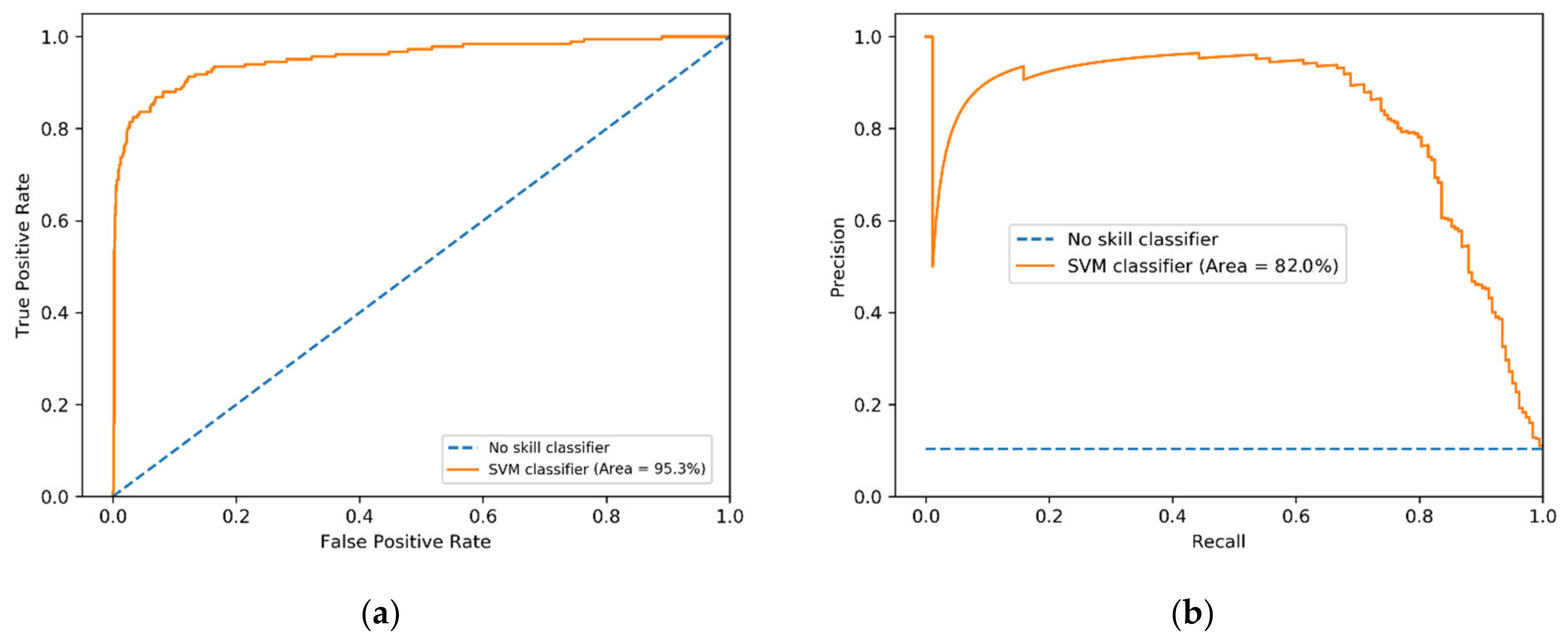
Figure 1. Examples of the Receiver Operating Characteristic (ROC) and Precision–Recall (PR) curves for an Support Vector Machine (SVM) applied to the same imbalanced dataset; (a) The ROC curve (AUC = 95.34) (b) The PR curve (AUC = 82.01).
Applsci 10 06253 g001
Figure 2. Design of the whole system for news classification and information extraction.
Applsci 10 06253 g002
Table 1. Threshold metrics to evaluate the imbalanced classification task
MetricFormula *Description
Sensitivity or recall R = T P T P + F N It is the fraction of positive patterns that are correctly classified. Under the presence of imbalanced classes, recall typically measures the coverage of the minority class.
Precision P = T P T P + F P It evaluates the proportion of correctly classified instances among the ones classified as positive. For imbalanced classification, it often calculates the accuracy of the minority class.
Specificity S = T N T N + F N It is used to measure the fraction of negative patterns that are correctly classified. It is only appropriate when false negatives are highly costly.
F-measure or F1-score F = 2 P R P + R It is the harmonic mean of precision and recall. The F1-measure is the most often used threshold metric for learning from imbalanced data.
* TP: True Positives; FP: False Positives; TF: False Negatives; and TN: True Negatives.
Table 2. Metrics calculated through 10-fold cross-validation for the five classifiers.
Folds
ClassifierMetric12345678910Average
CARTRecall0.6400.7720.6780.7220.6150.7230.7070.6110.6680.6520.679
Precision0.6760.7680.6710.7120.6570.6650.6920.7070.6580.6630.687
F measure0.6570.7700.6750.7170.6350.6930.6990.6550.6630.6570.682
ROC-AUC0.8030.8730.8180.8420.7890.8410.8360.7910.8150.8080.822
PR-AUC0.6760.7810.6930.7330.6560.7080.7130.6790.6800.6740.699
Compl. Naïve BayesRecall0.2310.2720.2290.2310.2300.2770.2870.2000.2510.2420.245
Precision0.9770.9801.0000.9800.9560.9271.0001.0000.9790.9560.976
F measure0.3740.4260.3730.3740.3710.4270.4460.3330.4000.3860.391
ROC-AUC0.9290.9610.9410.9420.9320.9250.9410.9300.9460.9360.938
PR-AUC0.7590.8310.7990.8130.7480.7310.8120.7740.8020.7510.782
kNNRecall0.0910.1300.1370.0610.0910.0380.0830.2210.0640.1010.102
Precision1.0000.8890.9661.0000.8950.7000.8820.9550.9230.9470.916
F measure0.1670.2270.2390.1160.1650.0720.1520.3590.1200.1830.180
ROC-AUC0.9270.9520.9150.9500.9310.9050.9280.9290.9190.9280.928
PR-AUC0.7970.8490.8130.8730.7690.7190.7860.8260.7760.8040.801
Random ForestRecall0.5590.6630.5560.5800.5720.5820.5690.5320.5720.5790.576
Precision0.9200.9460.9190.9760.8920.8920.9630.9350.9640.9360.934
F measure0.6960.7800.6930.7280.6970.7040.7150.6780.7180.7150.712
ROC-AUC0.9670.9790.9610.9710.9500.9510.9680.9630.9640.9630.964
PR-AUC0.8490.8960.8550.8850.8130.8140.8780.8320.8700.8480.854
SVMRecall0.5750.6680.5220.5470.5610.5600.5470.5110.6040.5620.566
Precision0.9550.9390.9730.9430.9380.9040.9520.9600.9500.9430.946
F measure0.7180.7810.6790.6930.7020.6910.6950.6670.7390.7040.707
ROC-AUC0.9630.9790.9490.9760.9470.9470.9670.9540.9550.9620.960
PR-AUC0.8310.9030.8670.8900.8270.7850.8720.8420.8650.8630.855
Table 3. Average of the metrics calculated through 10-fold cross-validation for both classifiers with sampling.
ClassifierSampling AlgorithmThreshold MetricsRanking Metrics
RecallPrecisionF-MeasureROC-AUCPR-AUC
SVMNone (Base version)0.56580.9456 *0.70690.95970.8545
SMOTE0.82780.75110.7873 0.96810.8485
Borderline SMOTE0.81950.76710.7921 *0.96610.8515
ADASYN0.83320.73760.78210.9687 0.8490
ROS0.85580.72170.78280.9693 *0.8561 *
RUS0.8596 †,§0.70740.77520.9693 *0.8550
Random ForestNone (Base version)0.57650.9355 †,§0.71290.96270.8552 †,§
SMOTE0.71140.88200.7872 §0.96390.8481
Borderline SMOTE0.70410.89170.78650.96240.8503
ADASYN0.71510.87490.78660.96330.8495
ROS0.67590.90500.77300.9647 §0.8429
RUS0.8641 *0.55230.67360.96210.8428
* the highest value of the metric; the second-highest value of the metric; § the highest value of the metric for a specific classifier.