Handling Skewed Data: A Comparison of Two Popular Methods

Abstract

Scientists in biomedical and psychosocial research need to deal with skewed data all the time. In the case of comparing means from two groups, the log transformation is commonly used as a traditional technique to normalize skewed data before utilizing the two-group t-test. An alternative method that does not assume normality is the generalized linear model (GLM) combined with an appropriate link function. In this work, the two techniques are compared using Monte Carlo simulations; each consists of many iterations that simulate two groups of skewed data for three different sampling distributions: gamma, exponential, and beta. Afterward, both methods are compared regarding Type I error rates, power rates and the estimates of the mean differences. We conclude that the t-test with log transformation had superior performance over the GLM method for any data that are not normal and follow beta or gamma distributions. Alternatively, for exponentially distributed data, the GLM method had superior performance over the t-test with log transformation.

1. Introduction

In the biosciences, with the escalating numbers of studies involving many variables and subjects, there is a belief between non-biostatistician scientists that the amount of data will simply reveal all there is to understand from it. Unfortunately, this is not always true. Data analysis can be significantly simplified when the variable of interest has a symmetric distribution (preferably normal distribution) across subjects, but usually, this is not the case. The need for this desirable property can be avoided by using very complex modeling that might give results that are harder to interpret and inconvenient for generalizing—so the need for a high level of expertise in data analysis is a necessity.

As biostatisticians with the main responsibility for collaborative research in many biosciences’ fields, we are commonly asked the question of whether skewed data should be dealt with using transformation and parametric tests or using nonparametric tests. In this paper, the Monte Carlo simulation is used to investigate this matter in the case of comparing means from two groups.

Monte Carlo simulation is a systematic method of doing what-if analysis that is used to measure the reliability of different analyses’ results to draw perceptive inferences regarding the relationship between the variation in conclusion criteria values and the conclusion results [1]. Monte Carlo simulation, which is a handy statistical tool for analyzing uncertain scenarios by providing evaluations of multiple different scenarios in-depth, was first used by Jon von Neumann and Ulam in the 1940s. Nowadays, Monte Carlo simulation describes any simulation that includes repeated random generation of samples and studying the performance of statistical methods’ overpopulation samples [2]. Information obtained from random samples is used to estimate the distributions and obtain statistical properties for different situations. Moreover, simulation studies, in general, are computer experiments that are associated with creating data by pseudo-random sampling. An essential asset of simulation studies is the capability to understand and study the performance of statistical methods because parameters of distributions are known in advance from the process of generating the data [3]. In this paper, the Monte Carlo simulation approach is applied to find the Type I error and power for both statistical methods that we are comparing.

Now, it is necessary to explain the aspects of the problem we are investigating. First, the normal distribution holds a central place in statistics, with many classical statistical tests and methods requiring normally or approximately normally distributed measurements, such as t-test, ANOVA, and linear regression. As such, before applying these methods or tests, the measurement normality should be assessed using visual tools like the Q–Q plot, P–P plot, histogram, boxplot, or statistical tests like the Shapiro–Wilk, Kolmogrov–Smirnov, or Anderson–Darling tests. Some work has been done to compare between formal statistical tests and a Q–Q plot for visualization using simulations [4,5].

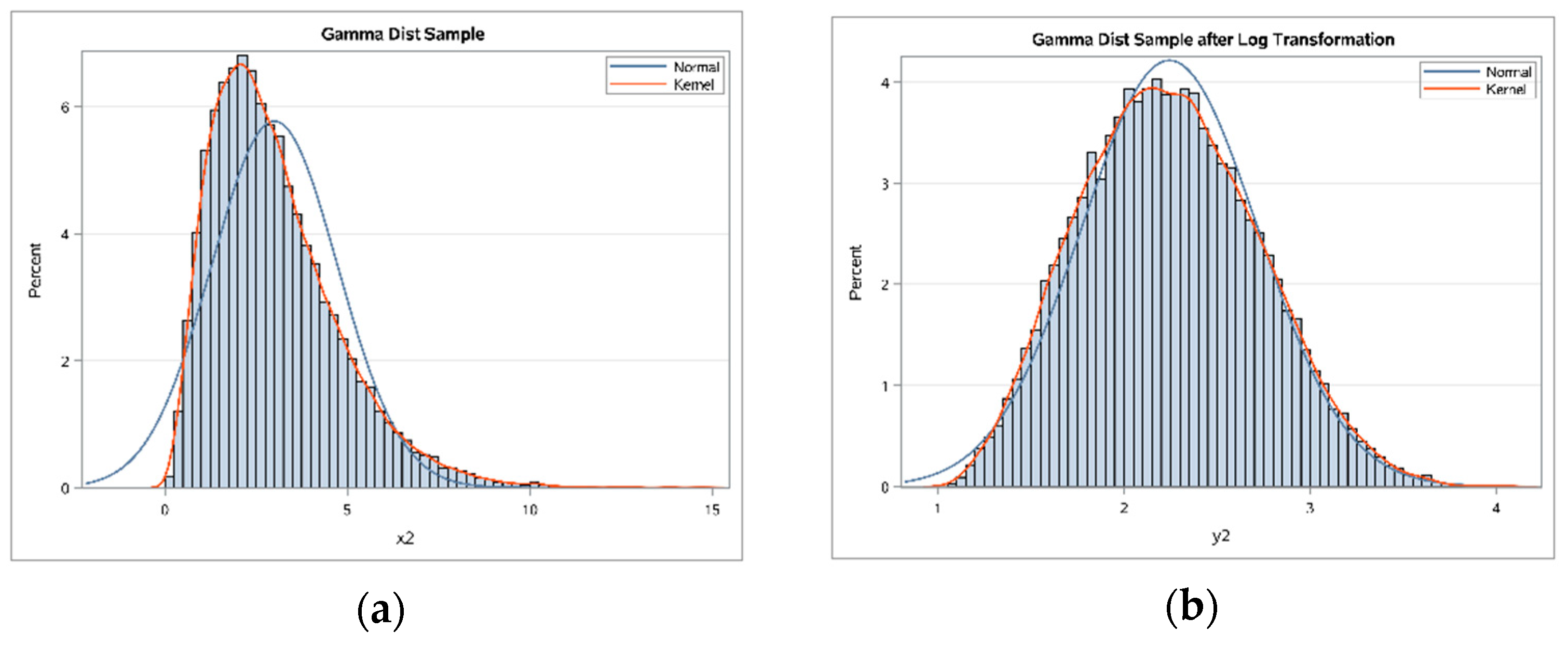
When testing the difference between two population means with a two-sample t-test, normality of the data is assumed. Therefore, actions improve the normality of such data that must occur before utilizing the t-test. One suggested method for right-skewed measurements is the logarithmic transformation [6]. For example, measurements in biomedical and psychosocial research can often be modelled with log-normal distributions, meaning the values are normally distributed after log transformation. Such log transformations can help to meet the normality assumptions of parametric statistical tests, which can also improve graphical presentation and interpretability (Figure 1a,b). The log transformation is simple to implement, requires minimal expertise to perform, and is available in basic statistical software [6].

Figure 1. Simulated data from gamma distribution before and after log transformation. (a) The histogram of the sample before the application of log transformation with fitted normal and kernel curves; (b) The histogram of the sample after the application of log transformation with fitted normal and kernel curves.

However, while the log transformation can decrease skewness, log-transformed data are not guaranteed to satisfy the normality assumption [7]. Thus, the normality of the data should also be checked after transformation. In addition, the use of log transformations can lead to mathematical errors and misinterpretation of results [6,8].

Similarly, the attitudes of regulatory authorities profoundly influence the trials performed by pharmaceutical companies; Food and Drug Administration (FDA) guidelines state that unnecessary data transformation should be avoided, raising doubts about using transformations. If data transformation is performed, a justification for the optimal data transformation, aside from the interpretation of the estimates of treatment effects based on transformed data, should be given. An industry statistician should not analyze the data using several transformations and choose the transformation that yields the most satisfactory results. Unfortunately, the guideline includes the log transformation with all other kinds of transformation and gives it no special status [9].

An alternative approach is the generalized linear model (GLM), which does not require the normality of data to test for differences between two populations. The GLM is a wide range of models first promoted by Nelder and Wedderburn in 1972 and then by McCullagh and Nelder in 1989 [10,11]. The GLM was presented as a general framework for dealing with a variety of standard statistical models for both normal and non-normal data, like ANOVA, logistic regression, multiple linear regression, log-linear models, and Poisson regression. The GLM can be considered as a flexible generalization of ordinary linear regression, which extends the linear modeling framework to response variables that have non-normal error distributions [12]. It generalizes linear regression by connecting the linear model to the response variable via a link function, and by permitting the magnitude of the variance of each measurement to be a function of its expected value [10].

The GLM consists of:

i

A linear predictor

$$\begin{array}{c}{\eta }_i={\beta }_0+{\beta }_1{x}_{1i}+\cdots +{\beta }_p{x}_{pi}=X\beta ,\end{array}$$

(1)

where ${\eta }_i, i=1,2,\dots ,N$, is a set of independent random variables called response variables, where each ${\eta }_i$ is a linear function of explanatory variables $x_j, j=1,\dots ,p$.

ii

A link function that defines how $E\left(y_i\right)={\mu }_i$ which is the mean or expected value of the outcome $y_i$, depends on the linear predictor, $g\left({\mu }_i\right)={\eta }_i$, where $g$ is a monotone, differentiable function. The mean $\mu$ is thus made a smooth and invertible function of the linear predictor:

$$\begin{array}{c}{\mu }_i= g^{-1}\left({\eta }_i\right),\end{array}$$

(2)

iii

A variance function that defines how the variance, $Var\left(y_i\right)$, depends on the mean $Var\left(y_i\right)=\varphi V\left({\mu }_i\right)$, where the dispersion parameter $\varphi$ is a constant. Replacing the ${\mu }_i$ in $V\left({\mu }_i\right)$ with $g^{-1}\left({\eta }_i\right)$ also makes the variance a function of the linear predictor.

In the GLM, the form of $E\left(y_i\right)$ and $Var\left(y_i\right)$ are determined by the distribution of the dependent variable $y_i$ and the link function $g$. Furthermore, no normality assumption is required [13,14]. All the major statistical software platforms such as STATA, SAS, R and SPSS include facilities for fitting GLMs to data [15].

Because finding appropriate transformations that simultaneously provide constant variance and approximate normality can be challenging, the GLM becomes a more convenient choice, since the choice of the link function and the random component (which specifies the probability distribution for response variable ($Y$) are separated. If a link function is convenient in the sense that the inverse-linked linear model of explanatory variables adheres to the support for the expected value for that outcome, it does not further need to stabilize variance or produce normality; this is because the fitting process maximizes the likelihood for the choice of the probability distribution for $Y$, and that choice is not limited to normality [16]. Alternatively, the transformations used on data are often undefined on the boundary of the sample space, like the log transformation with a zero-valued count or a proportion. Generalized linear models are now pervasive in much of applied statistics and are valuable in environmetrics, where we meet non-normal data frequently, as counts or skewed frequency distributions [17].

Lastly, it is worth mentioning that the two methods discussed here are not the only methods available to handle skewed data. Many nonparametric tests can be used, though their use requires the researcher to re-parameterize or reformat the null and alternative hypotheses. For example, The Wilcoxon–Mann–Whitney (WMW) test is an alternative to a t-test. Yet, the two have quite different hypotheses; whereas t-test compares population means under the assumption of normality, the WMW test compares medians, regardless of the underlying distribution of the outcome; the WMW test can also be thought of as comparing distributions transformed to the rank-order scale [18]. Although the WMW and other tests are valid alternatives to the two-sample t-test, we will not consider them further here.

In this work, the two-group t-test on log-transformed measures and the generalized linear model (GLM) on the un-transformed measures are compared. Through simulation, we study skewed data from three different sampling distributions to test the difference between two-group means.

2. Materials and Methods

Using Monte Carlo simulations, we simulated continuous skewed data for two groups. We then tested for differences between group means using two methods: a two-group t-test for the log-transformed data and a GLM model for the untransformed skewed data. All skewed data were simulated from three different continuous distributions: gamma, exponential, or beta distributions. For each simulated data set, we tested the null hypothesis ($H_0$) of no difference between the two groups means against the alternative hypothesis ($H_a)$ that there was a difference between the two groups means. The significance level was fixed at $\alpha =0.05$. Three sample sizes ($N=25, 50, 100$) were considered. The Shapiro–Wilk test was used to test the normality of the simulated data before and after the application of the log transformation. We applied two conditions (filters) on the data: it was only accepted if it was not normal in the beginning, and then it became normal after log transformation. The only considered scenarios were the ones with more than 10,000 data sets after applying the two conditions and the number of accepted simulated samples = T. We chose T to be greater than 10,000 to overcome minor variations attributable changing the random seed in the SAS code.

Afterward, a t-test was applied to transformed data, while a GLM model was fitted to untransformed skewed data. We used the logit link function when the data were simulated from a beta distribution, and we used the log link function when the data were simulated from the exponential distribution or gamma distributions. In each case, a binary indicator of group membership was included as the only covariate.

The two methods were compared regarding Type I error, power rates, and bias. To assess the Type I error rate, which is the probability of rejecting $H_0$ when $H_0$ is true, we simulated the two samples from the same distribution with the same parameters. The same parameters guaranteed statistically equal variances between groups, and thus we used the equal-variance two-sample t-test. In addition, the GLM method with an appropriate link function was used. If the p-value was less than the two-sided 5% significance level, then $H_0$ was rejected and a Type I error was committed (since $H_0$ was true). The Type I error rate is then the number of times $H_0$ was rejected (K for t-test and K_GLM for GLM) divided by the total number of accepted simulated samples (K/T or K_GLM/T).

To assess the power rate, which is the probability of rejecting $H_0$ when $H_{\mathrm{a}}$ is true and it is the complement of the Type II error rate, we assumed different mean values for the two groups by simulating the two groups from distributions with different parameters. In this case, since the variances are functions of the mean parameter as well, the unequal variance two-sample t-test was used. In these situations, if the p-value was less than the 5% significance level, then we rejected $H_0$ knowing that $H_{\mathrm{a}}$ is true. If the p-value was larger than the significance level, we failed to reject $H_0$ and concluded that a Type II error was committed (because $H_{\mathrm{a}}$ was true). Then, the power rate is the number of times $H_0$ was rejected (K for t-test and K_GLM for GLM) divided by the total number of accepted simulated samples (K/T or K_GLM/T). Each case (sample size, distribution, mean relationship) was repeated five million times (denoted as T₀). The diagram of testing the Type I error algorithm is shown in Figure 2.

Figure 2. Simulation and Hypothesis Testing algorithm (for Type I error, we simulated data from distributions with the same means, and for power, we simulated data from distributions with different means).

Regarding the difference estimates, other methods work on the response differently. The log transformation changes each response value, while the GLM transforms only the mean response through the link function. Researchers tend to transform back estimates after using a t-test with transformed data or after using GLM. We wanted to test which method gives a closer estimate to the actual difference estimates. So, while testing Type I error, we transformed back the estimates of the mean difference of the log-transformed data and the GLM-fitted data. Then we compared it with the means difference of the original untransformed data (which should be close to zero under (H₀) to see which of the two methods gave mean difference estimates that are not significantly different from the estimates of the actual mean difference. We also compared the estimates of the difference of the standard deviations between the log-transformed and the original data under the assumption that H₀ is true (while testing Type I error), so we could use pooled standard deviation.

In three applications to real-life data, we applied the two methods to determine whether the methods give consistent or contradicting results. By using visual inspection for this simulation study, Q–Q plots were used to test the normality of the data before and after the application of the log transformation to make sure that targeted variables were not normal before transformation and then became normal after transformation. After that, we used the t-test. Then, we used the bias-corrected Akaike information criterion (AICc) after fitting different continuous distributions to determine which distribution and link function to use with the GLM model [19,20]. Finally, we compared the results from both models. We generated all simulated data and performed all procedures using SAS codes. Moreover, the data that support the findings in the real-life applications of this study are openly available from the JMP software.

3. Results

3.1. Comparisons between the Two Methods

Comparisons were made between log-transformed t-tested data and original GLM-fitted data regarding the following aspects.

3.1.1. Comparison Regarding Type I Error Rates

Table 1 shows the parameters and the results of the alpha values for testing gamma-distributed data using the t-test and GLM, where α₁ represents the Type I error rate for the simulated data that was log-transformed and then tested using a two-group t-test assuming equal variances. Furthermore, α₂ represents the Type I error rate for the same groups of simulated data tested using GLM for gamma distribution with the log link function. Note that the Type I error rates for both methods are close to alpha = 0.05, but the t-test method is closer (0.0499 to 0.0503 in t-test data and 0.049 to 0.0577 in GLM data). In about 86% of the simulations, the t-test gave lower alpha values than the ones in the GLM. For the other 14% where the GLM gave lower Type I error, though, the t-test gave Type I error rates that were close to 0.05.

Table 1. Alpha values for gamma-distributed data tested using t-test and GLM.

Example	Sample Size	Parameters (Shape, Scale) 1	t-Test Alpha (α1)	GLM Alpha (α2)	Diff. = α1 − α2
1	25	2, 1	0.0501	0.0490	0.0011
2	50	2, 1	0.0502	0.0499	0.0003
3	100	2, 1	0.0502	0.0499	0.0003
4	25	3, 2	0.0501	0.0526	−0.0024
5	50	3, 2	0.0502	0.0512	−0.0010
6	100	3, 2	0.0500	0.0507	−0.0007
7	25	5, 1	0.0501	0.0555	−0.0054
8	50	5, 1	0.0499	0.0526	−0.0027
9	100	5, 1	0.0500	0.0517	−0.0018
10	25	4, 0.25	0.0503	0.0549	−0.0046
11	50	4, 0.25	0.0503	0.0536	−0.0033
12	100	4, 0.25	0.0502	0.0516	−0.0014
13	25	6, 3	0.0501	0.0562	−0.0062
14	50	6, 3	0.0501	0.0533	−0.0031
15	100	6, 3	0.0500	0.0517	−0.0017
16	25	9, 0.5	0.0502	0.0577	−0.0075
17	50	9, 0.5	0.0500	0.0535	−0.0035
18	100	9, 0.5	0.0500	0.0516	−0.0016
19	25	3, 0.5	0.0501	0.0529	−0.0029
20	50	3, 0.5	0.0501	0.0514	−0.0012
21	100	3, 0.5	0.0501	0.0511	−0.0010

¹ The two simulated groups have the same parameters.

Table 2 contains summary information for the Type I error results for the gamma, exponential and beta distributed data. For the exponentially distributed data examples, the Type I error rates for the GLM across all parameter values were lower than the t-test rates in all of the settings, though the t-test Type I error rates did not exceed 0.0504 (0.0497 to 0.0504 for the t-test; 0.0367 to 0.0477 for the GLM). The t-test Type I error rates for beta distributed outcomes were lower than those from the GLM in all settings (0.0497 to 0.0511 for the t-test; 0.0518 to 0.0589 for the GLM). Figure 3 shows the Type I error for both methods, which are compared to 0.05 for the three distributions.

Table 2. Summary of Type I error rates for gamma, exponential and beta distributed data tested using the t-test and GLM.

Dist.	t-Test			GLM
	Average α	Min α	Max α	Average α	Min α	Max α
Gamma	0.0501	0.0499	0.0503	0.0525	0.0490	0.0577
Exponential	0.0502	0.0497	0.0504	0.0432	0.0367	0.0477
Beta	0.0503	0.0497	0.0511	0.0544	0.0518	0.0589

Figure 3. Type I error rates for the t-test and GLM compared to 0.05 for the three distributions.

3.1.2. Comparison Regarding Power

Table 3 presents the parameters and power results for the beta-distributed data. P₀ is the power values calculated for the two-group t-test using the information provided by knowing the two distributions and their parameters that are used in the simulation process, P₁ is the empirical power of the two-group t-test conducted on the log-transformed groups, and P₂ is the empirical power of the GLM-fitted data. Here we note that the GLM power rates were higher than those for the t-test with log transformation in 68% of the settings with absolute values of differences ranging from 0 to 0.0884. In 74% of the settings, the GLM power rates exceeded or equalled the calculated power, while the t-test power rates exceeded the calculated power in only 58% of the settings. Although the percentage of GLM power rates that exceeded or equalled the computed power was higher than the percentage of t-test power rates, the estimated power rates produced by the t-test were not that different to those that were produced by the GLM, with a difference of less than 0.1.

Table 3. Power values for beta distributed data tested using the t-test and GLM: P₀ is the power value of the two-group t-test calculated prior to the simulations, P₁ is the empirical power of the two-group t-test conducted on the log-transformed groups, and P₂ is the empirical power of the GLM-fitted data.

Example	Sample Size	Group1 Shape Parameters (α, β)	Group2 Shape Parameters (α, β)	Original t-Test Power (P0)	t-Test Power (P1)	GLM Power (P2)	Power Diff. = P1 − P2
1	25	5, 3	5, 5	0.792	0.8217 2	0.8531 2	−0.0314
2	50	5, 3	5, 5	0.977	0.9815 2	0.9858 2	−0.0043
3	100	5, 3	5, 5	>0.999	0.9998 2	0.9999 2	−0.0001
4	25	2, 3	0.5, 0.5	0.224	0.1158	0.2042	−0.0884
5	25	2, 3	1, 3	0.75	0.7633 2	0.7532	0.0101
6	50	2, 3	1, 3	0.965	0.9552	0.9456	0.0095
7	25	2, 5	1, 3	0.108	0.1262 2	0.1142 2	0.0120
8	50	2, 5	1, 3	0.17	0.2071 2	0.1718 2	0.0352
9	25	2, 2	2, 5	0.967	0.9637	0.97392	−0.0102
10	50	2, 2	2, 5	>0.999	0.9995 2	0.9997 2	−0.0002
11	100	2, 2	2, 5	>0.999	1.0000 2	1.0000 2	0.0000
12	25	2, 3	2, 2	0.371	0.3909 2	0.4318 2	−0.0409
13	50	2, 3	2, 2	0.645	0.6374	0.6723 2	−0.0350
14	100	2, 3	2, 2	0.912	0.8824	0.9021	−0.0197
15	25	2, 3	2, 5	0.586	0.5948 2	0.6321 2	−0.0373
16	50	2, 3	2, 5	0.876	0.8599	0.8788 2	−0.0189
17	100	2, 3	2, 5	0.993	0.9874	0.9903	−0.0029
18	25	1, 3	2, 2	0.985	0.9822	0.9828	−0.0005
19	50	1, 3	2, 2	>0.999	0.9998 2	0.9998 2	0.0000

² Power exceeds the original t-test expected power P₀.

Table 4 contains summary information for the power results of gamma, exponential and beta distributed data tested using both methods. In about 86% of the exponentially distributed data examples, the power for the GLM was higher than that for the t-test, with absolute values of differences ranging from 0.001 to 0.108. Moreover, in 41% of the settings, GLM power rates exceeded or equalled the calculated power. Then again, in just 10% of the settings, t-test power rates exceeded the calculated power, while in the gamma-distributed data examples, the power for the GLM was higher in about 85% of the settings, with absolute values of differences ranging from 0.000 to 0.363. In addition, in 41% of the settings, GLM power rates exceeded or equalled the calculated power. Still, in just 15% of the settings, t-test power rates exceeded the calculated power. Figure 4 shows powers for both methods compared to the computed power rates for three distributions.

Table 4. Summary of power values for exponential and gamma-distributed data tested using the t-test and GLM: P₀ is the power value of the two-group t-test calculated prior to the simulations, P₁ is the empirical power of the two-group t-test conducted on the log-transformed groups, and P₂ is the empirical power of the GLM-fitted data.

Dist.	Difference between t-Test Power and Calculated Power			% $\ge$ P0	Difference between GLM Power and Calculated Power			% $\ge$ P0	Difference between GLM Power and t-Test Power
	Average	Min	Max		Average	Min	Max		Average	Min	Max
Gamma	−0.106	−0.299	0.000	15%	0.033	−0.017	0.119	95%	0.138	0.000	0.363
Exponential	−0.040	−0.113	0.049	1%	0.005	−0.148	0.095	59%	0.044	−0.035	0.108
Beta	−0.003	−0.108	0.037	53%	0.009	−0.020	0.061	74%	0.012	−0.035	0.088

Figure 4. Power rates for the t-test and GLM compared to the computed power rates for the three distributions.

3.1.3. Comparison Regarding Estimates of Mean Differences and Standard Deviations

Next, we compared the estimates of the mean difference between the log-transformed data, the GLM-fitted data and the original untransformed data under testing Type I error, simulating every two groups from the same distribution to ensure the mean difference will be close to zero. For all the tested sampling distributions, we transformed back the estimates of the transformed mean differences and they were not significantly different from the actual mean differences according to p-values. On the contrary, we transformed back the estimates of the mean differences in the GLM according to the link function in each scenario and all were significantly different from zero. Table 5 presents the parameters and the back-transformed estimates’ values of mean differences of log-transformed and GLM-fitted exponentially distributed data.

Table 5. Mean differences estimates’ values for original, log-transformed and GLM-fitted exponential distributed data.

Example	Sample Size	Scale Parameter	Actual Difference	Back Transformed Trans. Mean Diff.	p-Value	Back Transformed GLM Mean Diff.	p-Value
1	25	1	0.0001	0.0131	1	1.0306	<0.0001
2	50	1	0.0011	0.0066	1	1.0135	<0.0001
3	25	1.5	0.0000	0.0202	1	1.0331	<0.0001
4	50	1.5	0.0004	0.0095	1	1.0149	<0.0001
5	25	2	−0.0003	0.0263	1	1.0363	<0.0001
6	50	2	−0.0002	0.0123	1	1.0162	<0.0001
7	25	3	−0.0004	0.0364	1	1.0396	<0.0001
8	50	3	0.0009	0.0086	1	1.0188	<0.0001
9	100	3	0.0002	0.0037	1	1.0084	<0.0001
10	25	2.5	−0.0004	0.0151	1	1.0381	<0.0001
11	50	2.5	0.0003	0.0073	1	1.0178	<0.0001
13	25	3.5	−0.0004	0.0151	1	1.0381	<0.0001
14	50	3.5	0.0006	0.0095	1	1.0195	<0.0001
15	100	3.5	−0.0023	0.0040	1	1.0083	<0.0001
16	25	6	−0.0002	0.0267	1	1.0425	<0.0001
17	50	6	0.0002	0.0131	1	1.0206	<0.0001
18	100	6	−0.0007	0.0130	1	1.0084	<0.0001

Finally, we compared the estimates of the standard deviation between the log-transformed data and the original skewed data. According to the resulting p-values, the estimates of the pooled standard deviation of the log-transformed data were significantly smaller than the estimates of the pooled standard deviation of the original skewed data in all the tested examples, as expected. Table 6 presents the parameters and the estimates values of standard deviation for the original and log-transformed gamma-distributed data. This component, however, was not provided by the GLM procedure.

Table 6. Standard deviation estimates for the original and log-transformed gamma-distributed data.

Example	Sample Size	Parameters (Shape, Scale)	Two-Group t-Test between SD(x1) and SD(y1)
			Trans. Mean	Actual Mean
1	25	2, 1	0.8839	1.4017
2	50	2, 1	0.8767	1.3931
3	100	2, 1	0.87	1.3878
4	25	3, 2	1.0554	3.518
5	50	3, 2	1.0456	3.4678
6	100	3, 2	1.045	3.4814
7	25	5, 1	0.72	2.313
8	50	5, 1	0.7135	2.2487
9	100	5, 1	0.7116	2.2406
10	25	4, 0.25	0.4167	0.5086
11	50	4, 0.25	0.4088	0.4941
12	100	4, 0.25	0.4062	0.4898
13	25	6, 3	0.7747	7.6397
14	50	6, 3	0.7695	7.4241
15	100	6, 3	0.7657	7.4052
16	25	9, 0.5	0.487	1.567
17	50	9, 0.5	0.484	1.5254
18	100	9, 0.5	0.482	1.5037
19	25	3, 0.5	0.6107	0.8733
20	50	3, 0.5	0.6023	0.8558
21	100	3, 0.5	0.6003	0.8534

3.2. Application to Real-Life Data

In this section, we present three examples of real-life data that we imported from JMP software and tested using both of our studied methods.

3.2.1. The Lipid Data

We have real data from 95 subjects at a California hospital and are interested in whether triglyceride levels differ between patients considering their gender. The data were observed to be skewed and fitted to gamma distribution according to AICc values. The Q–Q plot and the frequency histogram of the untransformed and log-transformed lipid data are presented in Figure 5. Using the t-test after log transformation, we got a t-value of $t_{58.47}= 2.56$ with a p-value = $0.0065$, indicating a significant difference between the two gender means, with the male triglyceride average larger than the average for females. An application of the GLM to the original data with gamma distribution and log link function yielded a p-value $=0.006$. For this data, the results from the t-test of log-transformed data and the GLM both indicated evidence of a difference in triglyceride means between males and females.

Figure 5. The normal Q–Q plots (up) for the Triglycerides variable before and after transformation and the frequency histogram of the Triglycerides variable on the left (down) is fitted with a gamma distribution (green).

3.2.2. The Catheters Data

We have real data from a sample of 592 children who received multiple attempts to start peripheral IV catheters in the inpatient setting. The data were obtained from a study conducted at two southeastern US hospitals from October 2007 through October 2008 [21]. We are interested in checking the difference in children’s weight between children who lost IV vs. those who did not. The weight variable was skewed and fitted to a gamma distribution according to AICc values. The Q–Q plot and the histogram of the untransformed and log-transformed weight variable are given in Figure 6.

Figure 6. The normal Q–Q plots (up) for the weight variable before and after transformation and the frequency histogram of the weight variable on the left (down) fitted to a gamma distribution (red).

Then, the t-test after log transformation was used; we got $t_{394.29}= -3.39$ with a p-value = $0.0004$, indicating a significant difference between the two groups; the average for the children who lost the IV weight was lower than that of the other group, who did not lose the IV. An application of the GLM to the original data with gamma distribution and log link function returned a p-value $=0.0042$. For this data, the results from the t-test with log-transformed data and the GLM indicated evidence of a difference in mean for the weight variable.

3.2.3. The Pharmaceutical and Computer Companies Data

We have a data table of 32 registered companies and some information like the sales, profits, assets, and number of employees in each company. There are two types of companies, computer companies and pharmaceutical companies. We wanted to check if the assets variable is significantly different between the two types. So, we tested the mean difference between the computer and pharmaceutical groups regarding the assets variable. The data was found to be skewed and fitted to an exponential distribution according to AICc values. The Q–Q plot and the frequency histogram of the companies’ untransformed and log-transformed data are presented in Figure 7.

Figure 7. The normal Q–Q plots (up) for the Assets variable before and after transformation and the frequency histogram of the Assets on the left (down) fitted to an exponential distribution (red).

We tested the data using both methods. The resulted t-value is $t_{29.99}=1.97$ with p-value $=0.0292$, which indicates that there is a significant difference between the two groups’ means and that the pharmaceutical companies have a significantly higher assets mean than the computer companies. For the second method, we applied GLM to the original data with a log link function. The resulting p-value $=0.4908$ indicates that there is no significant difference between the assets’ means of the two types of companies. So, the two methods gave contradicting results and this issue puts us on a crossroads. We need to decide which result to adopt.

4. Discussion

In this work, we compared the use of a t-test on log-transformed data and the use of GLM on untransformed skewed data. The log transformation was studied because it is one of the most common transformations used in biosciences research. If such an approach is used, the scientist must be careful about its limitations; especially when interpreting the significance of the analysis of transformed data for the hypothesis of interest about the original data. Moreover, a researcher who uses log transformation should know how to facilitate log-transformed data to give inferences concerning the original data. Furthermore, log transformation does not always help make data less variable or more normal and may, in some situations, make data more variable and more skewed. For that, the variability and normality should always be examined after applying the log transformation.

On the other hand, GLM was used because other nonparametric tests’ inferences concern medians and not means. In addition, GLM models deal differently with response variables depending on their population distributions, which provides the scientist with flexibility in modeling; GLM allows for response variables to have different distributions, and each distribution has an appropriate link function to vary linearly with the predicted values.

Each comparison was made for two simulated groups from several sampling distributions with varying sample sizes. The comparisons regarded Type I error rates, power rates and estimates of the means. Overall, the t-test method with transformed data produced smaller Type I error rates and closer estimations. The GLM method, however, produced a higher power rate compared to t-test methods, though both reported acceptable power rates.

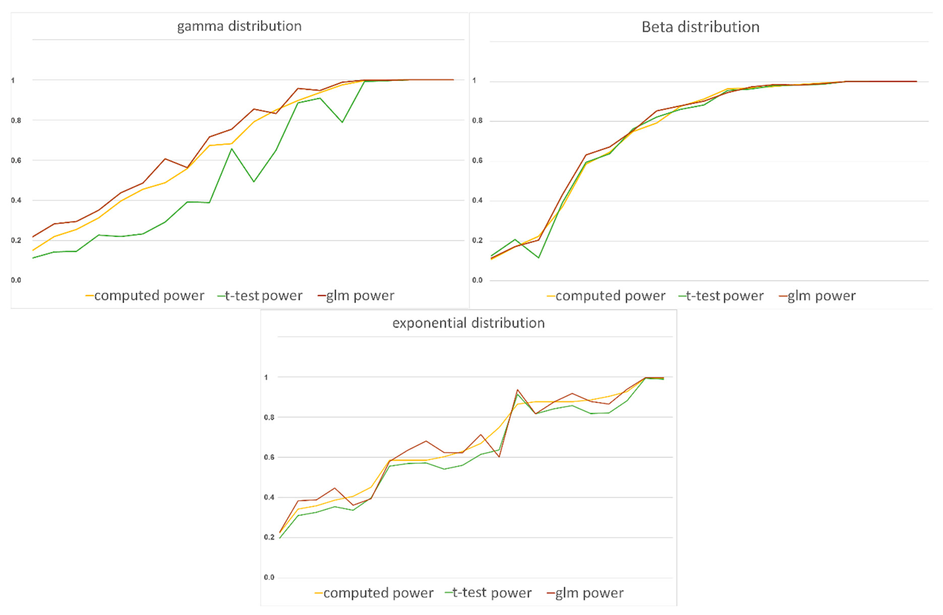
For gamma distribution, Type I error rates in the t-test case were very close to 0.05 (0.0497 to 0.0504), while the Type I error rates of the GLM method had a wider range (0.0490 to 0.0577). For most examples in the gamma-distributed data, the Type I error rates of the t-test method were smaller than the respective rates in the GLM method. Regarding power, the GLM rates were higher in about 85% of the settings than the ones using the t-test, with absolute values of differences, ranging from 0.000 to 0.363.

The back-transformed estimates of the mean differences in the t-test case were not significantly different from the estimates of the original data mean differences in the t-test method. The GLM estimates, in contrast, were significantly different from the estimates of the original data. So, if we are looking for lower Type I error and closer estimates, we can use the t-test method with transformed data. However, if we are looking for a method with higher power rates, we recommend choosing the GLM method.

In the exponentially distributed data, the GLM method has achieved a noticeably lower Type I error rate and higher power in most of the settings than the t-test method. Regarding the estimates, the t-test method gave closer estimates. Despite the closer estimates for the t-test method, our advice is to use the GLM method.

For beta distributed data, Type I error rates seem to favor the t-test method with transformed data. The power rates of the GLM method were higher than the power rates in the t-test method, with absolute values of differences ranging from 0 to 0.0884. Furthermore, by looking at Figure 4, we can see that the two methods have very close power rates. So, both methods seem to be good enough in this matter. Nevertheless, since the t-test method has lower Type I rates and closer estimates in the beta distributed data, we recommend it over GLM.

The missing rates for some of the parameters’ combinations, especially in calculating power rates, are due to two reasons. First, in most cases, rates were not missing, but the counts for accepted simulated samples were less than 10,000. That caused the setting to be rejected. Particularly in the case of calculating power rates, the two groups are from the same distribution with different parameters, which made it harder to apply the two filters (both groups should not be normally distributed before the use of log transformation and normally distributed after the application of log transformation). Although being less than 10,000 caused the estimates to vary as a response to changing the random seed, it gave the same conclusion. For example, if the GLM had a higher power rate in one sitting of parameters, it kept having a higher power rate even if we changed the seed. Yet, we preferred not to include these settings because we needed the estimates to be reproducible.

Second, in rare cases, none of the samples’ normality issues were resolved with log transformation, so we had zero accepted simulated samples. As a result, our comparison does not apply to that parameter combination. In conclusion, we did not consider missing rates as an issue since GLM had a higher power rate, as well as the t-test had closer mean difference estimates in all other accepted settings.

Our results were consistent across parameter settings and sample sizes ($N=25, 50, 100$), so we expect that the difference in sample sizes will not affect the method choice no matter what the sample size effect is over the method performance itself.

After analyzing the data from our real-life examples, we recommend reporting the results from the t-test with log-transformed data for the lipid data example and catheters data example, since the best fit for both examples was a gamma distribution. Because the catheters data example had larger sample size (n = 592) than used in our simulations, we conducted additional simulations with sample size of 296 per group. Though not reported, these results concurred with our reported findings at lower sample sizes.

We followed the same steps for the third example (the pharmaceutical and computer data example), which had the exponential fit as the best fit. We conducted additional (though not reported) simulations with 16 subjects per group, and again observed results that agreed with our reported findings. Thus, our recommendation is to report the GLM method results.

Therefore, for any Bio-application research, studying the appropriate statistical distribution that fits the dependent variable can help us to determine if a parametric model can reasonably test the data after log transformation is used. Alternatively, it would probably be better to abandon the classic approach and switch to the GLM method.