1. Introduction
Prostate cancer (PCa) remains one of the most commonly diagnosed solid organ tumor types among men. Early diagnosis and an active follow-up can allow improved prognosis and prevent life-threatening conditions. Once the decision of treatment has been taken, having the most complete information for treatment and follow up is crucial. In 2020, there will be approximately 1,806,590 cancer cases diagnosed and 606,520 cancer deaths are projected to occur in the United States. This classification has been reported by the ICD-O, excepting childhood and adolescent cancers, which were classified according to the ICCC [
1]. On the other hand, PCa is the third predicted cause of death in EU with 78,800 death in 2020 [
2]. This entails a rate estimation of 10.0/100,000 men.
Medical support systems used to assist in the diagnosis of prostate lesions generally focus on prostate segmentation [
3,
4,
5,
6]. They rely on computerized techniques for prostate cancer detection applied to ultrasound, magnetic resonance and computed tomodensitometric images [
7]. For example, Vos et al. [
8] used 3D-T2 imaging to define a specific Region of Interest (ROI), which was subsequently used on diffusion- and perfusion-weighted images to extract relevant features. MRI has been established as the best imaging modality for the detection, localization and staging of PCa on account of its high resolution and excellent spontaneous contrast of soft tissues and the possibilities of multi-planar and multi-parametric scanning [
9]. Among the techniques used to detect PCa, MRI also allows non-invasive analysis of the anatomy and the metabolism in the entire prostate gland.
Furthermore, many recent works confirm that the combination of several MRI techniques facilitates the evaluation of prostate diagnoses according to the PI-RADS classification, both for radiologists and medical experts [
10]. For instance, a thorough evaluation of various prostate cancer studies was presented in [
11]; this study highlights that the correct localization of ROI-containing tumor tissue as the most prevalent problem encountered in the diagnosis of a prostate cancer and other related tasks. Traditionally, clinical experts use different software tools to validate the diagnoses and make annotations in several files. This approach is far from being efficient when managing and dealing with abundant medical data. For the reasons stated above, we propose a new software tool to provide support for the time consuming segmentation process used for annotating images in the clinical practice. Additionally, it enables radiologists to make use of novel semi-automatic segmentation techniques instead of the traditional manual segmentation approaches.
The contributions of this paper are two-fold: we introduce a novel prostate cancer segmentation graphical user interface on which several segmentation algorithms can be easily implemented. In order to demonstrate the strengths and the potential applications of the proposed tool, we included several segmentation algorithms with the software:
We implemented a modified version of the snake-based active contours segmentation (ACS) algorithm presented in [
12] to work with prostate images, which we will refer as
Basic ACS.
A simplified version of the Basic ACS algorithm, referred as Simplified ACS, is included with the program, that runs faster, but with less accuracy.
Finally, we extended the Basic ACS model in order to integrate a Gradient Vector Flow (GVF) component to improve the segmentation process, which we will refer as GVF ACS in this paper.
The extensions of original algorithm, in tandem with the novel graphical user interface greatly simplify the segmentation process as it enables a boosted semi-automatic interaction with the clinicians who, eventually, can validate the correctness of the ROI generated by the different methods. Finally, a quantitative study to validate the correctness of the generated segmentation compared to the ground truth and the algorithms is provided. It is worth to mention that the developed program serves as an initial version of a tool that we hope, will create a lot of opportunities to contribute with newer algorithms or improvements to the existing ones in the field of prostate segmentation.
The rest of this paper is organized as follows: in
Section 2 we introduce the used dataset and we explain the implementation and features of the proposed Graphical User Interface. Then we describe the Basic ACS and the modifications we introduced to make it work in prostate images. Finally, we present details about the Gradient Vector Flow (GVF) model and its implementation into our tool. In
Section 3, we include a single experimental case study to demonstrate the advantages of the proposed approach. In
Section 4 we discuss the results in the light of the clinical perspective, and in
Section 5 we present the conclusions as well as future works.
2. Materials and Methods
In this section we present the source database and the main contributions of the article, namely the proposed GUI for prostate segmentation process and later on, the integration of the Basic ACS model and its extensions using GVF, the GVF ACS model.
2.1. Database and ROIs References
A database with prostate MRI, based on clinical data with tumor and healthy cases was used. The examinations used in our study contained three-dimensional T2-weighted fast spin-echo (TR/TE/ETL: 3600 ms/143 ms/109, slice thickness:
mm) images acquired with sub-millimetric pixel resolution in an oblique axial plane. Each study comprises a set of 64 slice images. This database was used in previous works [
11] and it has been facilitated for testing the software.
The ground truth annotations were performed using the ProstateAnalyzer tool [
11], that allows the drawing of an annotation in a given MRI. For this task, experts with more than 10 years of experience on prostate imaging were asked to provide the annotations using the tool. All the dataset and ground truth data are provided from the medical imaging department of the University Hospital of Dijon (France). The institutional committee on human research approved the study, with a waiver for the requirement for written consent, because MRI and MRSI were included in the workup procedure for all patients referred for brachytherapy or radiotherapy.
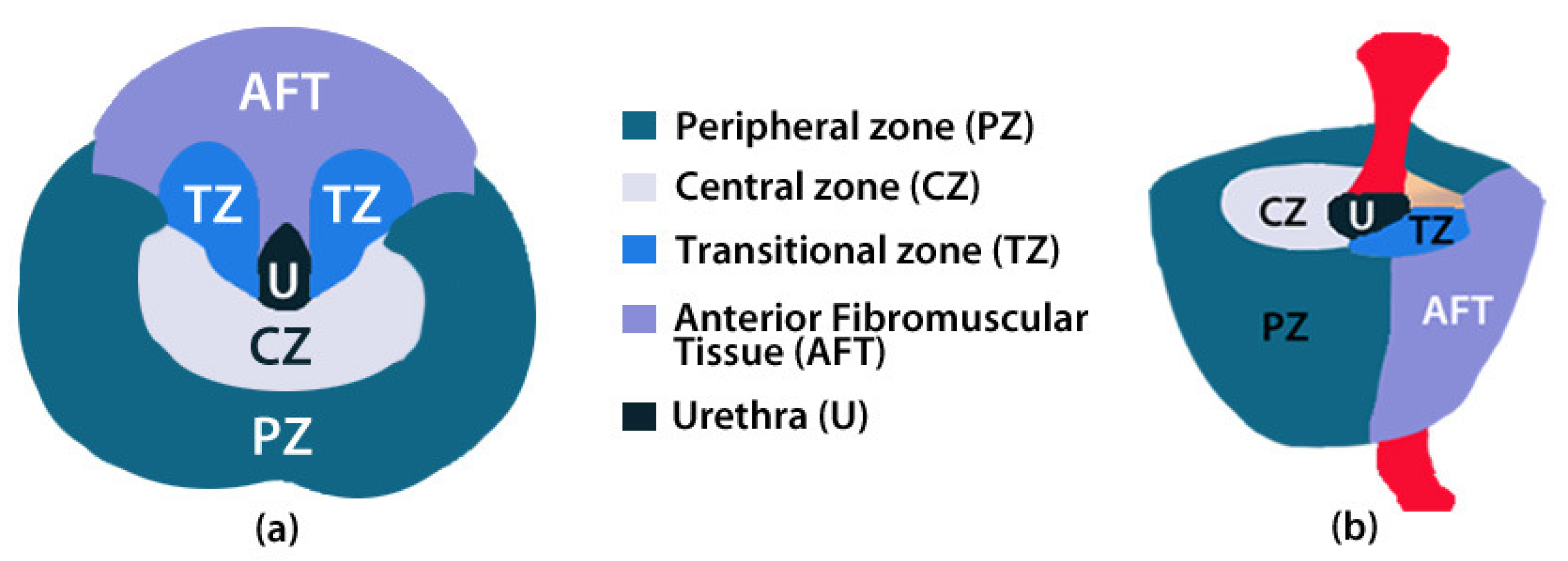
The prostate is composed of a peripheral zone (PZ), central zone (CZ), transitional zone (TZ) and an anterior fibromuscular tissue (AFT) depicted in
Figure 1. Most cancer lesions occur in the peripheral zone of the gland, fewer occur in the TZ and almost none arise in the CZ. A detailed description of the influence of the prevalence factor risk according the prostate zone is described in [
13]. The T2WI modality was chosen because it provides the best depiction of the prostate’s zonal anatomy.
The PZ represents up to 70% of a normal prostate gland and around 75% of prostate cancers originate in this zone. The CZ represents about 25% of a normal healthy prostate gland in young adults. Even though the frequency of cancers originating here is much lower, they tend to be of the more aggressive type [
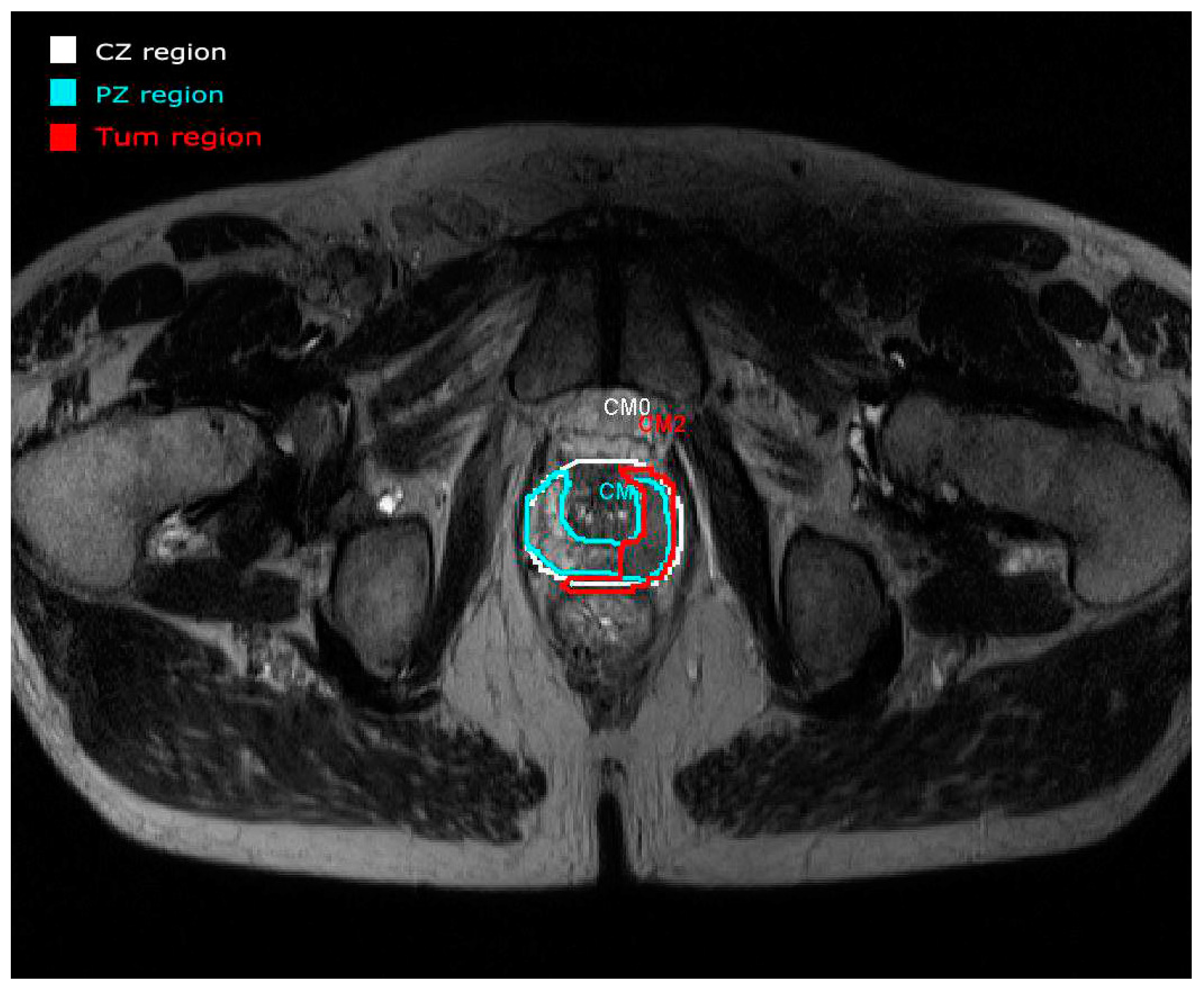
14]. An example of a real study case provided by the panel visualization of the prostate tool [
11] is depicted in
Figure 2. All the overlays are annotated with manual drawings made by radiologists. Each region is represented by different colors (CZ in white and PZ in blue) focusing on a tumor area represented in red (Tum). This example shows the importance of making annotations in regions of interest. In this case, a manual segmentation is validated by experts.
Therefore, one of the main motivations of this work is to develop a new tool focused on improving the results of this initial manual segmentation using Active Contour Models (ACM), facilitating the task of the experts.
In order to attain the above-mentioned goals, we have implemented a novel Graphical User Interface that permits to import, analyze and annotate prostate MR images. The program requires an initial annotation from the user, that does not require to be perfect, and the outcome is an annotation more accurate than the initial one. The modular design of the software allows for integrating segmentation methods as plug-ins or extensions that can be used for testing and clinical purposes. Additionally, this design enables easy performance comparisons between already integrated methods and new methods. In what follows, we will discuss the design of this GUI and subsequently, we will present a study case using three implementations of an ACS model for segmenting the different prostate sections in MR images. It is important to note that this tool and the developed algorithms have not yet been clinically tested and the results presented here represent a proof of concept. However, for the design of the GUI, the expertise and suggestions of clinical experts have been taken into account.
2.2. Implementation of the Graphical User Interface for Prostate Segmentation
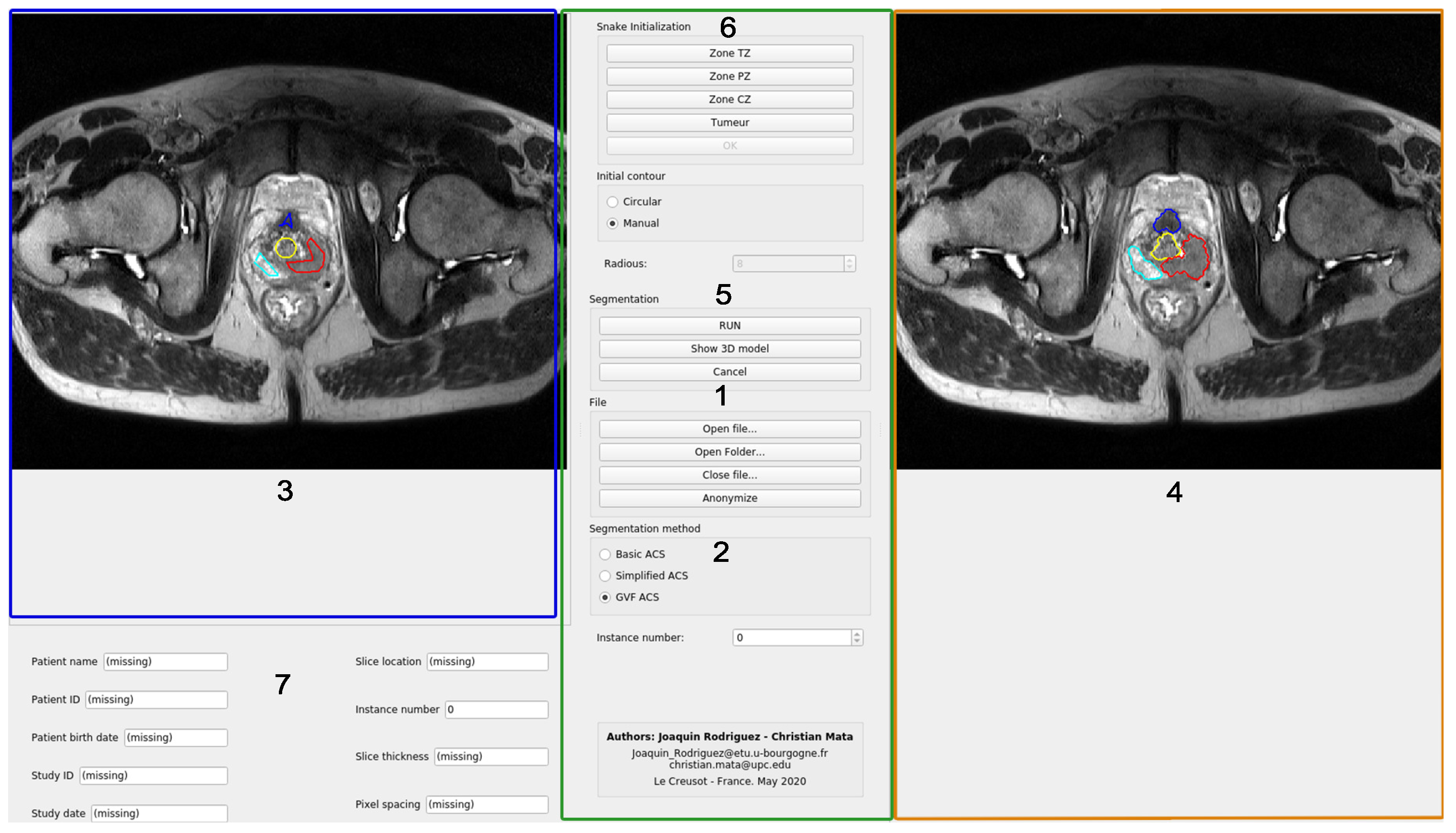
In this section, the code organization and the user interface of the program will be explained. The main window of the program is shown in
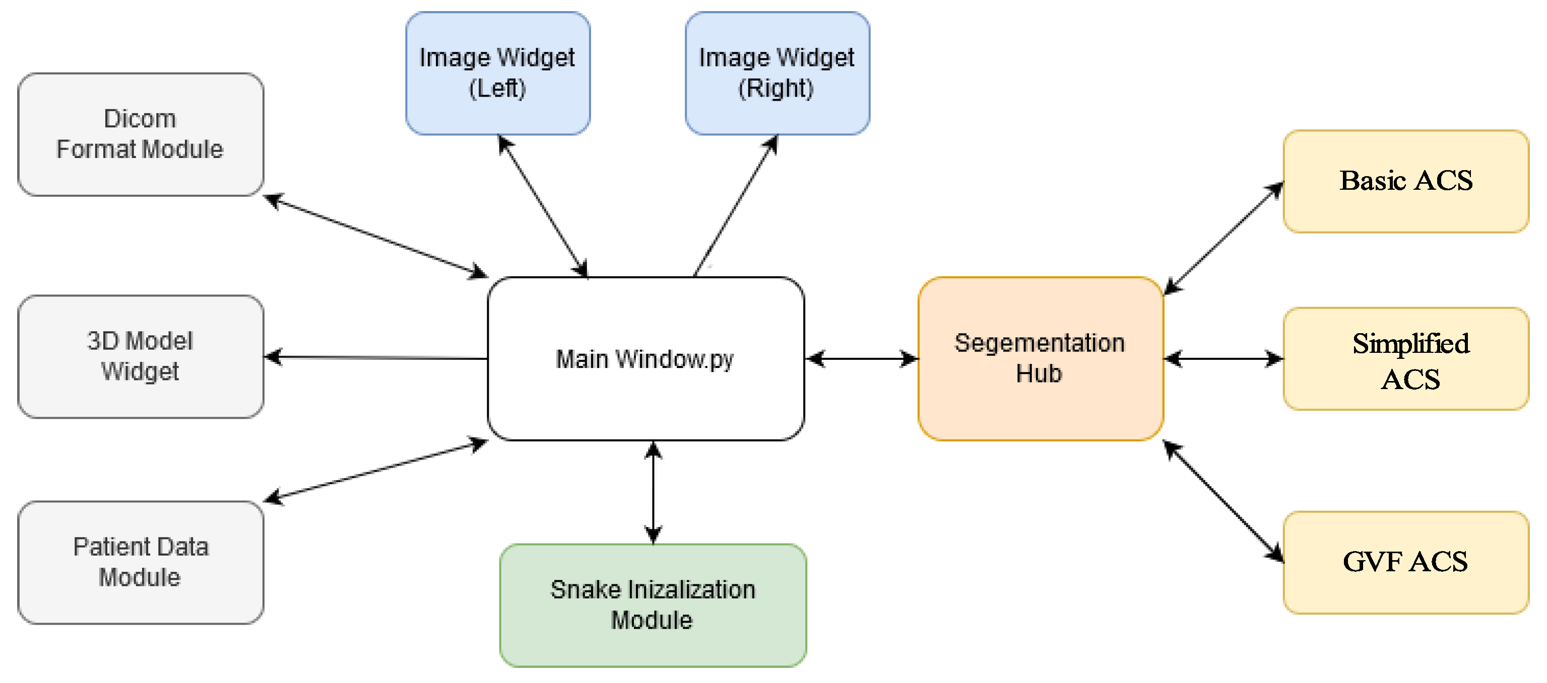
Figure 3. All the code has been developed in Python, using the modules PyQt for the user interface and PyDicom to open the files included in the testing dataset. The code has been organized in modules that do not interact with each other. The integration of all of them has been made in the Main Window class.
Each module is placed in folders as follows:
DICOM. This module contains the code that is in charge of handling the Digital Imaging and Communication On Medicine (DICOM) formatted files. It can open either a folder or a single DICOM image. Each file is assumed to contain only one image. The read information will be stored locally on RAM, and after the file or files has/have been opened, a signal will be emitted, and the information can be requested as many times as the user wants.
The data available to the user includes the images and the patient data fields. This module is also in charge of anonymizing the files and writing them into disc. The functionalities of this module can be accessed through the buttons in the Section 1 of the
Figure 3.
Image segmentation. This module stores all the Python code related to the segmentation procedure. The main class in this module is Segmentation-Hub, which is in charge of selecting the right class for the object that will produce the segmentation, according to the method chosen by the user. The selection of the segmentation method can be done in Section 2 of
Figure 3. By implementing the methods in this manner, the actual implementation of the segmentation task is completely transparent for other classes that make use of this module. To select certain segmentation method, only a label that defines the method must be provided.
This module also contains two other files with useful functions:
Image widget. This module is in charge of showing the image, as well as the initial and the resulting contours from the segmentation. The same module is used for both, left and right images. It also captures the clicks from the user to generate either the circular or the manual initial contour. Both types of initialization will be explained later. The image widget is represented in Sections 3 and 4 of
Figure 3.
Model 3D widget. It shows a 3D representation of the output segmentation, based on the Python module Matplotlib. This process is relatively simple as it only replicates the given contour vertically. If the spatial resolution is given in the input DICOM file, the scale of the axis will be given in millimeters. It can be accessed through the button
located in Section 5 of
Figure 3.
Snake init widget. This widget is in charge of handling all the functionalities of the Snake initialization group, placed at the top of the central control panel of the application.
Each button will request the main window to ask the user to enter the initial contour in the left image. Once the user has finished, the gathered contours are returned back to this module.
Afterwards, the corresponding masks for those contours can be generated for the snake algorithm (the mask consists of an image with values of 1 in the interior of the contour, and zeros outside of it). The interface for this module is represented in Section 6 of
Figure 3.
User data widget. It is implemented as an efficient and easy to use manner to handle all the user information as an object, and to show it. This class stores all the information related to the patient or the study, retrieved from the DICOM file. It also contains the corresponding widgets that are shown below the left image area, where the gathered information is displayed (see Section 7 of
Figure 3).
A block diagram of the proposed tool components is depicted on
Figure 4.
Finally, regarding the user interface showed in
Figure 3, this program has four well-defined sections:
Left panel. In this area (highlighted in blue), the loaded images are shown, and the user can draw the initial contours of the snake of the different areas of the prostate. Each prostate zone is surrounded with a different color to make it easily distinguishable (see
Figure 3)
Right panel. This area (highlighted in orange) shows the loaded images, and the results of the evolution of the selected snake algorithm. Each prostate zone has a pre-defined color, and they match with the colors used for the initial contours (see Section 4 of
Figure 3).
Bottom area. The patient information retrieved from the DICOM file is shown (highlighted in blue). Moreover, information related to the spatial resolution and thickness of the gathered slice are included (Section 7 of
Figure 3)
Central area. This is the control panel area (highlighted in green). All the functionalities and possible configurations of the program are located in this area. It is represented in the Sections 1, 2, 5 and 6 of
Figure 3.
To the best of our knowledge, tools as the proposed in this work, which integrate a Graphical User Interface and semi-automated segmentation algorithms for image annotation do not exist (at least not for prostate MR images). Therefore, a preliminary effort to develop a GUI that includes several active contour model implementations is very important and has driven the development of this work. On the other hand, from the implementation point of view, this program represents an excellent tool to deploy new snake-based algorithms: given that the initial contour and the original image are available in the Segmentation-Hub module, new algorithms can be created using Python, and added as an standalone file to the Image Segmentation folder. This procedure will add another option to the GUI, and the new algorithm’s performance and accuracy can be compared with the already existing techniques. This code-base is now available as a GitHub repository to the community [
15].
In order to demonstrate how different segmentation methods can be integrated into the proposed tool, we have implemented various versions of an Active Counter Model within the Image Segmentation module of our tool. These methods have been included not only for demonstration purposes, but also to serve as a baseline for future developments in prostate MRI segmentation research (people can improve them, or develop new methods based on them). The proposed Active Contour Model, to be discussed in the following section, also represents a novel contribution, as it has not been previously reported to be used for prostate segmentation purposes.
2.3. Implementation of the Proposed Active Contour Model
The base method implemented is inspired on [
12,
16]. Both of them are active contours—level-set algorithms. Particularly, the model by Pluempitiwiriyawej et al. [
12] was conceived and customized to work with MR images. The general idea of snake algorithms is to modify a curve based on certain forces that push the boundaries of such curve until it reaches the border of the object of interest. A particular feature of this type of segmentation algorithm is that they are unsupervised methods, given that there is not feedback on whether the boundary is following the correct borders or not. Due to this assumption of snake-based methods, an initial contour must be provided, and the closer this initial contour is to the real object, the better the result of the segmentation.
Typically, most snake-based algorithms follow the information about the gradient of the image, which means the curve will try to evolve towards the edges of the object. Nonetheless, if the object does not contain well defined edges, or it has been previously smoothed in order to reduce the noise, this algorithm might fail in following the shape of the object. As a consequence, the outcome will be either a contour that is smaller or larger than the object’s boundaries, or in the worst case, the contour will be reduced until it disappears. This is the reason why several researchers developed specific algorithms depending on the type of object to detect, and the type of image to deal with. This is done adding different terms called . Each constraint added to the algorithm defines a prior, and its corresponding weight will define its contribution to the force.
In this previous work [
12], the goal is to segment the shape of the left ventricle of the heart, but since it is aimed to work with MR images, and the priors are similar to the assumptions that can be done for the prostate zones, we considered it as a good starting point for carrying out our experiments and implement the GVF extension to demonstrate its viability in this image modality. The basic assumption of the developed algorithm is that the contour will split the image into two areas, the target object and the background. The evolution of the curve will be driven trying to minimize an energy functional that in this case, it is composed of four components. Each of them will define the priors the final contour must comply with [
12]:
Model matching. it is assumed that the pixel values inside and outside the object follow different statistical models, specified as and , respectively.
Edge information. the contour must be attracted to certain clues that describe the limits of the object, i.e., the strongest edge values of the image should attract the curve.
Shape prior. Besides certain possible variations between patients, each prostatic zone has a general shape. This shape information can be thought as a function , with . The parameters define a model of the actual shape and size of the requested zone, and depending of how distant is the contour from this estimated shape, this prior will contribute more or less to the snake evolution.
Contour smoothness: The contour is supposed to not be jagged or too noisy, so this parameter controls that.
Then the functional that defines the energy described above, depending on the contour
C, can be expressed as:
where
are the weights of each prior included in the energy function. This function will be used to make evolve the contour. It follows that it is possible to transform the information of the contour in a level set function, i.e., the information about the contours can be expressed as a function, where the pixels that belong to the object have certain value (or level), the background ones have another level, and the frontier, which is the contour
C, is represented by another level. In the case of this paper, the contour is expressed through the level set function as in Equation (
2). As it can be seen, the contour is in the level where the function
is equal to zero.
represents the space of the image.
Then, the energy functional can be expressed as depending on
.
This function evolves with each iteration (i.e.,time), depending on the direction in which the forces push the contour. In the following sections the particularities of each term will be described.
2.3.1. Region-Based Model Matching—Term
The aim of this term is to split the image space into two regions that contain homogeneous pixels: the object and the background. Let’s call them and , respectively. These two regions are separated by the contour C. An homogeneous region implies a region where all the pixels that are contained in it are described by the same stochastic model. The points that belong to the object have intensities , and they are described by the model , and the ones that belong to the background have values , and they are represented by the model .
The idea of the model is as follows: let’s consider the image
to be formed by two regions, of piecewise-constant intensities
and
, and that the intensities of the object are represented by
. The boundary of this region is
. Then, the pixel values of the image
are
inside
, and
outside of it. Given this, it is possible to build the following fitting term:
where
C is any variable curve, and
and
are two constants that depend on the contour
C. Based on the previous explanation, if
C =
, then
is approximately zero, because each distance between the image value and the constant
are approximately zero for each region. If the curve
C is outside
, then its interior contains parts of the object and parts of the background, while the exterior of
C contains only elements of the background. Because of this,
and
. In the backwards case, i.e., the contour
C is smaller than
, the outside contains parts of the object and the background, whilst the inside only contains parts of the object. It follows that
and
. Finally, this fitting function can be used to find the boundaries of the object, by minimizing its value such as
In order to achieve this boundary, the evolution of the curve
C is done by moving pixels from the exterior to the interior of the contour, and vice-versa. The first estimation of the energy function for this prior is in Equation (
6):
where
p is the probability density function of the image intensities
u, given the contour
C, and the models
and
. Over these probabilities, it is assumed that each element, object and background, are statistically independent, and they have pdfs
and
, respectively. Moreover, the pixel intensities are considered to be independent from each other. With these assumptions, and taking the negative of the logarithm of the pdfs, the Equation (
6) becomes Equation (
7).
Assuming a continuous function, the contour embedded in the zero level-set function
, and considering the Heaviside function in order to create a single integral over all the domain of the image, the Equation (
7) can be generalized as shown in Equation (
8).
It is assumed that both elements in the image follow a Gaussian distribution, with means and , and variances and , which are unknowns, and for each contour C, they will be estimated.
2.3.2. Edge-Based Function—Term
This term will push the contour towards the edges of the object. The computation of this type of force is done through the edge-map
generated from the image
. The most common implementation is the gradient of the smoothed image.
where
is a Gaussian kernel of parameter
, ∇ is the gradient operator and (.) ⁎ (.) is the convolution operator. Finally, the energy functional, depending on the level set function
, which corresponds to this prior is given by the Equation (
10).
where
will return non-zero values only for the pixels that are on the contour
C.
2.3.3. Object Shape Prior—Term
This term has been introduced in [
12] to reinforce an elliptical shape in heart MR images, but it can be changed by any other shape model depending on the specific object to be segmented. The addition of this prior will improve the performance of the general active contour implementation. For instance, if the target to segment has a circle-like shape, then the snake function can be constrained to satisfy an ellipse equation. In that case, the functional corresponding to this energy term can be defined as
where
is the ellipse distance function defined as:
The parameters
are computed in such a way that the cloud of points around the contour
C fits with this ellipse equation. This means that the parameters of
must be computed for each contour
C, and they will change the force direction in order to minimize this distance function. Finally, introducing the level set function
, where the contour
C is embedded, the shape prior is computed as in Equation (
12), when integrating in all the space
.
2.3.4. Contour Smoothing—Term
Finally, it is desirable that the generated contour is smooth. This can be achieved if the Euclidean arc length of the contour
C is minimized. It follows that the contribution function for this prior is the one represented in Equation (
13).
It is worth mentioning that if only this term is included in the functional, the shape of the contour will become a circle, and then it will start shrinking until it eventually disappears. Nonetheless, when all the terms are put together, this situation is avoided, and the effect is to smooth the curve. Again, adding the level set function where the contour is embedded, the final function for
is defined in Equation (
14).
The following step is to combine all the functional together, and expand the minimization problem, in such a way the function
, which contains the contour
C as its level zero, evolves towards the edge of the object. The entire procedure is well explained in [
12], and it consists of three tasks:
Define the statistical model constants, in such a way that they comply with the prior that the pixel distribution follows a Gaussian distribution.
Estimate the ellipse parameters to obtain the distance functional contribution.
Define the contour evolution equation. This can be done by applying the Euler-Lagrange (EL) equation to the functional of the four priors. Then, considering that
is a function of time, the
equation is equaled to the derivative of
with respect to the time. The resulting function is given in Equation (
15).
where
,
are the stochastic models of the object and the background, respectively,
is the curvature of the contour,
is our level set function, and
is the potential function.
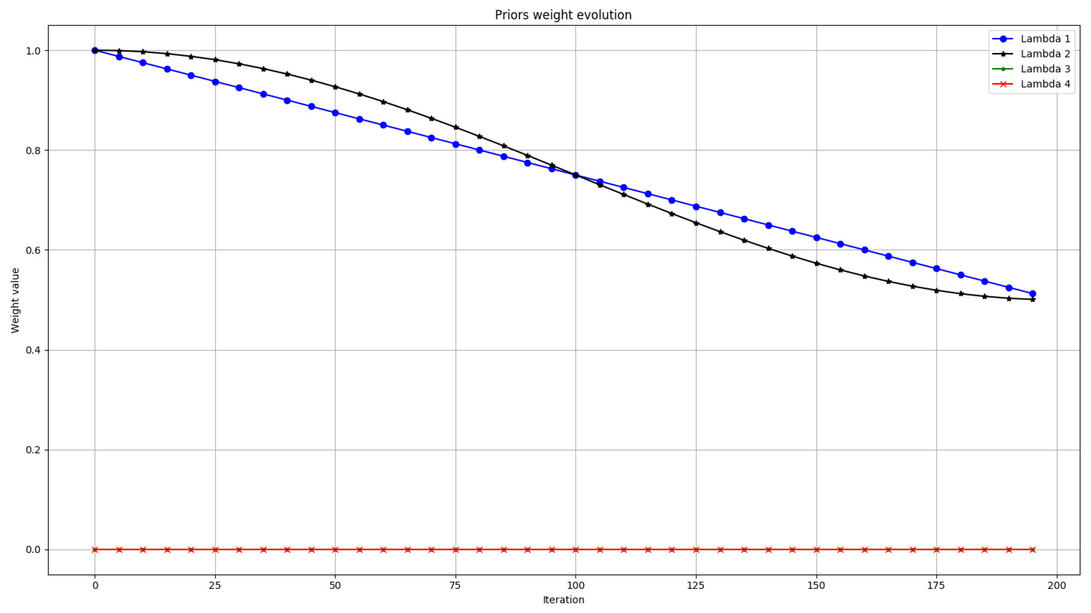
The different values of , , and will define the contribution of the corresponding energy term, from to , and the one with the biggest value will enforce its properties over the others. In practice, the parameters setting is done empirically, and there is no rule that defines how to chose them. It depends on the quality and the properties of the input image. One solution is to make the weights to evolve at each iteration to obtain the best results. The general idea of this evolution is that at the beginning, the algorithm should minimize the energy functional trying to cover all the object, pushing the boundaries towards the edges (effect produced by and ), and when the algorithm is close to the end, the curve must enforce the shape of the contour and its smoothness ( and ).
For the particular case of prostate segmentation, several objects with different shapes have to be considered. Therefore, the shape prior cannot be only an ellipse, as it happens in the case of the left ventricle of the heart. Thus for this implementation, the value of has been set to zero.
Additionally, through several experiments, we concluded that the contribution produced by the smoothness prior is not noticeable. In fact, it produces small variations in the contour, and the result is that the algorithm takes more time to converge. This is the reason why the value of
has been set to zero too. Finally, the suggested evolution of the weights is shown in
Figure 5.
2.4. Gradient Vector Flow Approach (GVF)
When dealing with snakes algorithms, there are two types of implementations:
Parametric Active Contours (PACs) or
Geometric Active Contours (GACs). They differ in how they define the curve function, since equations formulated for the minimization problem stays almost the same. PACs are based on a parametric curve of a shape represented in Equation (
16):
with the constraint that it should be closed, i.e.,
. Geometric Active Contours, on the other hand, define the curve to be deformed as embedded in a level-set function, generally as its level zero. This last case is the one implemented and described in
Section 2.3. GACs have advantages over PACs, since they are computationally more stable and they are able to change their topology as the function is deformed. Nonetheless, the implemented method is an edge-based method, since it uses the gradient as pushing force, and local intensity information to determine if a pixel belongs to the object or not. Due to this, several problems can appear, such as:
If the edges of the object are not well defined, a leaking problem occurs, leading the snake outside of the object’s boundaries.
If the initial contour is not close to the limits of the object, the gradient will not be able to guide the snake to the edges of the object. If the image is just black and white with one object on it, an initial contour far away from the object will not evolve. On the other hand, if there are other objects around, the snake might be attracted to them, instead of the desired object.
Since the snake uses the local pixel information to determine the evolution of the curve, it is sensible to the image noise.
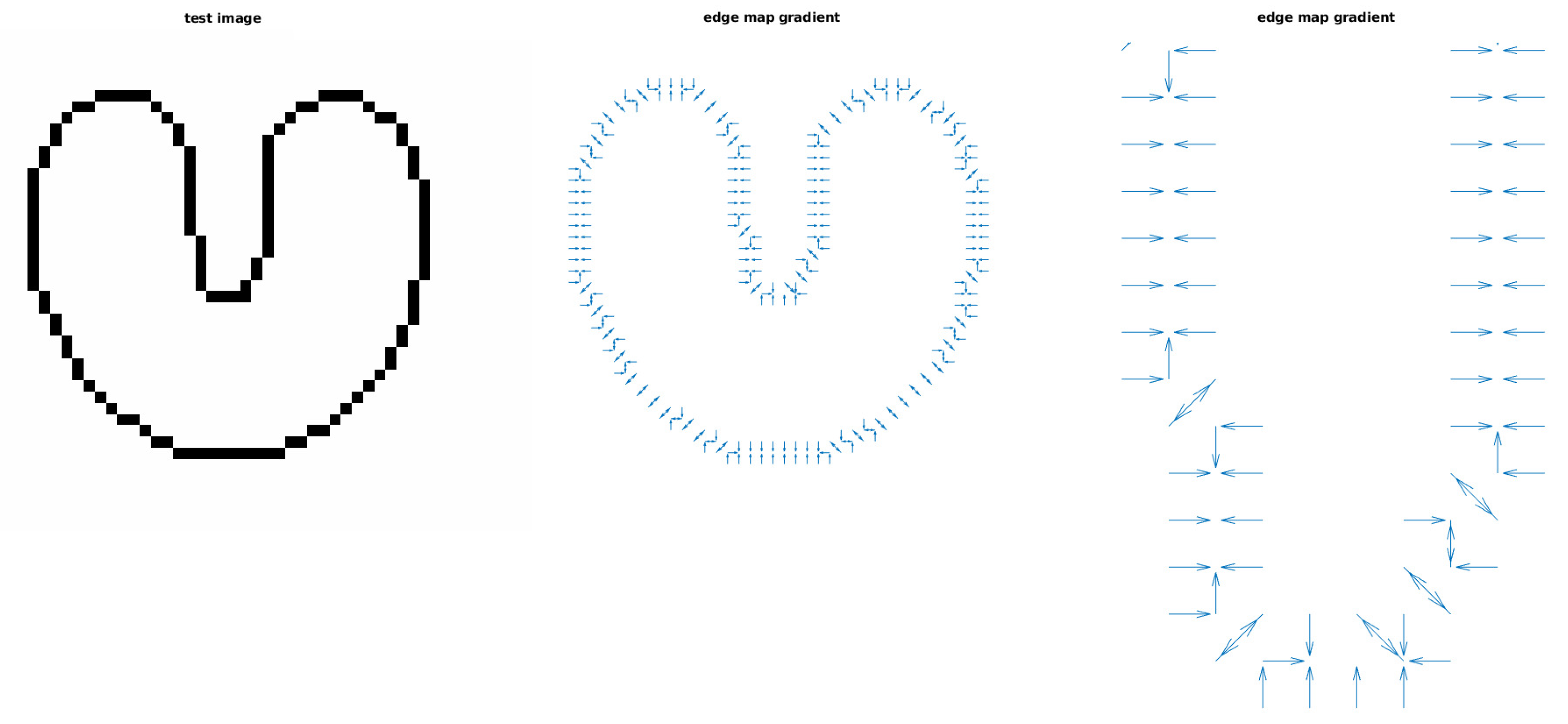
Additionally, the fact of using gradients only, brings another effect related to concavities, that is illustrated in
Figure 6.
In this case, a simple object with a narrow concavity, and its corresponding gradient vector field are shown. From it, it is easy to see that:
These last two problems can be solved in the previously explained algorithm with an external force that, not only adds vectors where the gradient is zero, but that also adds a downwards component in the long concavities in such a way that the active contour will be pushed to the interior of this type of areas. This external force is called Gradient Vector Flow (GVF) [
17]. Adding this component to the energy described in
Section 2.3 will help to not only make the system more robust against initialization effects, but it will improve the outcome by attaching the resulting snake really close to the edges of the object.
The GVF is a dense vector field
derived from the original image, and it is the result of minimizing the energy term defined in Equation (
17) [
17].
where
and
are the partial derivatives of
u and
v with respect to the variable
x, respectively,
and
are the partial derivatives of
u and
v with respect to the variable
y, respectively, and
is the edge map of the original image. The parameter
is a constant that serves as regularization: it adjusts the balance between the first and the second term of the integral, and it should be adjusted based on the noise. The higher the noise, the higher the value of
. Interpreting the energy term presented in (
17), it is possible to see that if the gradient of the edge map is too small, the energy term depends only on the partial derivatives of
u and
v. On the other hand, if this gradient is large, the integral is dominated by it, and the value of the GVF that minimizes the energy is
, i.e., the gradient vector flow is equal to the gradient of the edge map on those cases. It can be demonstrated that the vector field
that minimizes (
17) is the result of the decoupled pair of differential Equations (
18) and (
19).
where
is the Laplacian operator. Similarly as in Equation (
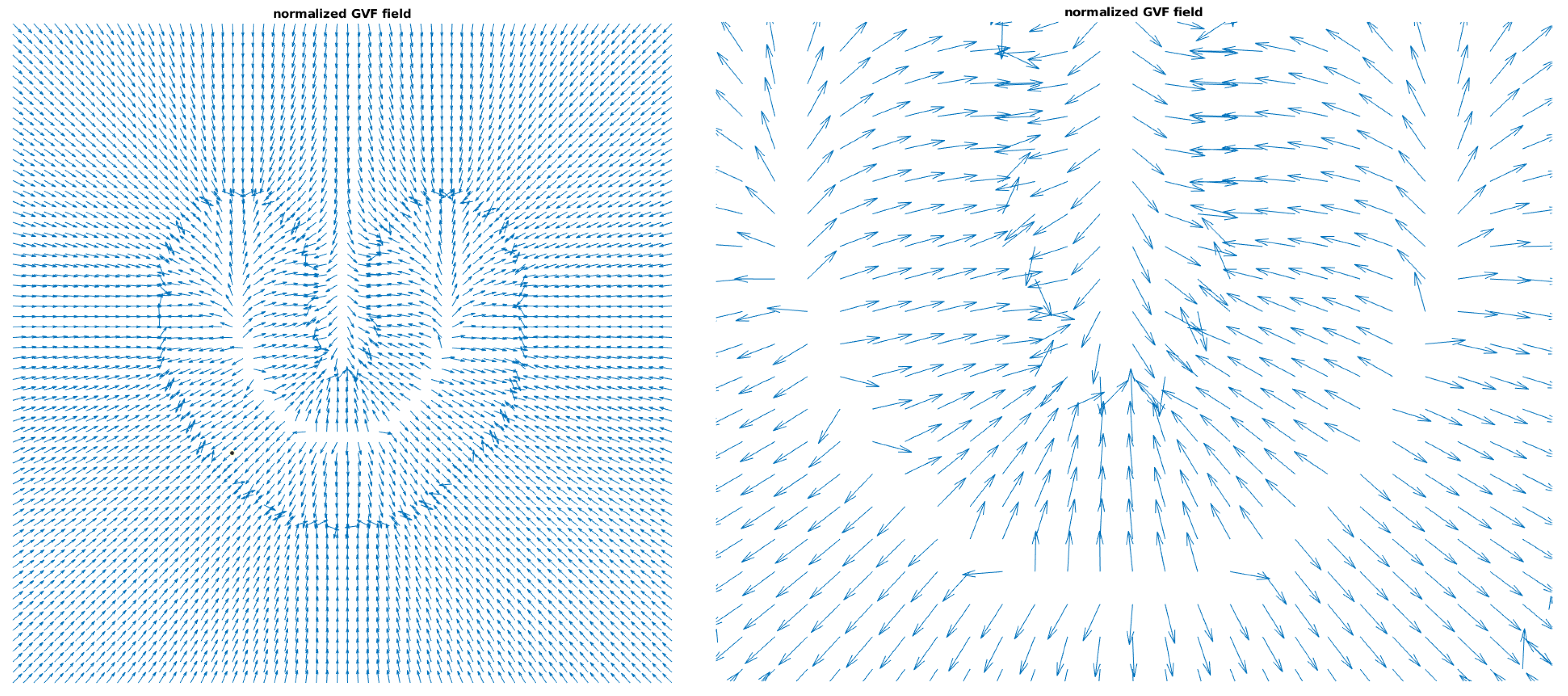
17), it is possible to see that in the regions where the gradient of the edge map is small, the solution of the differential equations for the GVF are the solution of Laplace’s equations. Furthermore, this solution is interpolated from the boundaries of the object, and that’s the reason why the resulting field, even far away from the object, points to the edges of it. The gradient vector flow of the same image as in
Figure 6, is shown in
Figure 7. Now, the solution to the Equations (
18) and (
19) provides vectors in the areas where the gradient is zero, and the vectors in the concavity contains downwards components too.
Once the GVF has been computed, it is fixed for the entire the image, and what remains is the optimization equation that will guide the deformation of the active contour to the edges of the object, based on this new force. Several researchers have been working on adding gradient vector flow to the traditional snake equations. For the implementation made in
Section 2.3, only GACs algorithms can be adapted to be added as an external force to the energy functional defined in the Equation (
15), as it has been done in [
18,
19]. A simplified version of the GVF optimization equation from [
19] is used, and defined as:
The parameter
regularizes the step size,
is the level-set function,
is the curvature,
is the Gradient Vector Flow vector field, and the parameter
regulates the balance between the two forces. The right hand factor of (
20) is added directly to Equation (
15), giving Equation (
21):
This new segmentation algorithm has been included in the list of options to segment the different prostate zones. After having implemented the Basic ACS in Python, the extension with a GVF component is trivial: all the components of this new force are already available in the code except for the vector field . Since this vector field is fixed for a given image, a new class has been created that solves the optimization problem for the GVF. This new piece of code is executed before the main loop of the segmentation algorithm. Since there are no rule for setting both and , we arbitrarily decided to set them to 1. In order to adjust the contribution of this new force, the factor has been introduced. For the following experiments, this factor has been also set to 1. In the coming sections, the graphical user interface result of the integration of all the modules will be showed. Then, the described algorithms will be tested to show their performance.
3. Experimental Case of Use for Demonstration
In this section a case of use for demonstration is presented. Previously, the proposed GUI has been explained in
Section 2.2. A detailed definition of this algorithm and the introduced improvements have been explained in
Section 2.3 and
Section 2.4. The following study case demonstrates how an user can use the proposed tool to manage and segment a real prostate image.
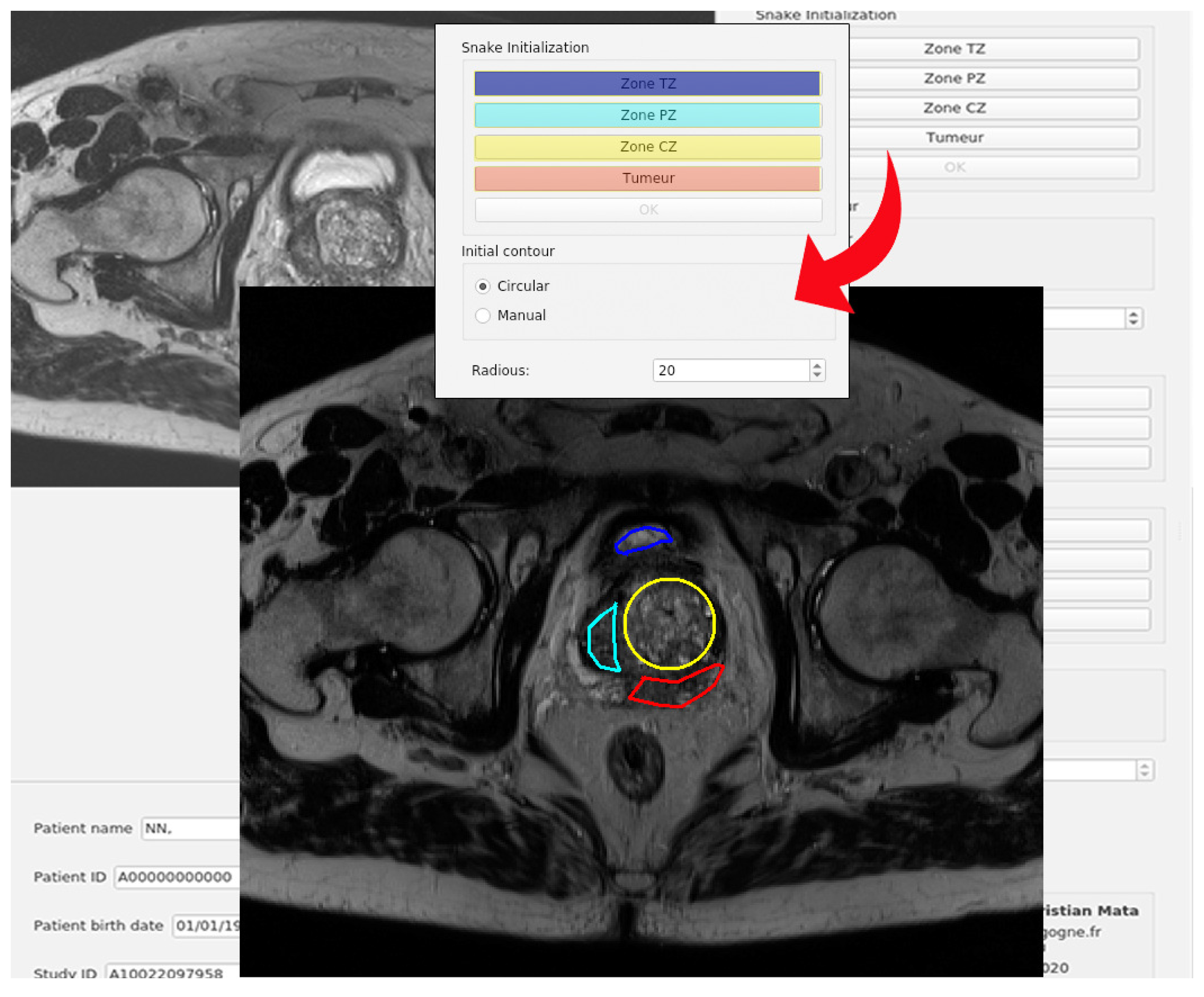
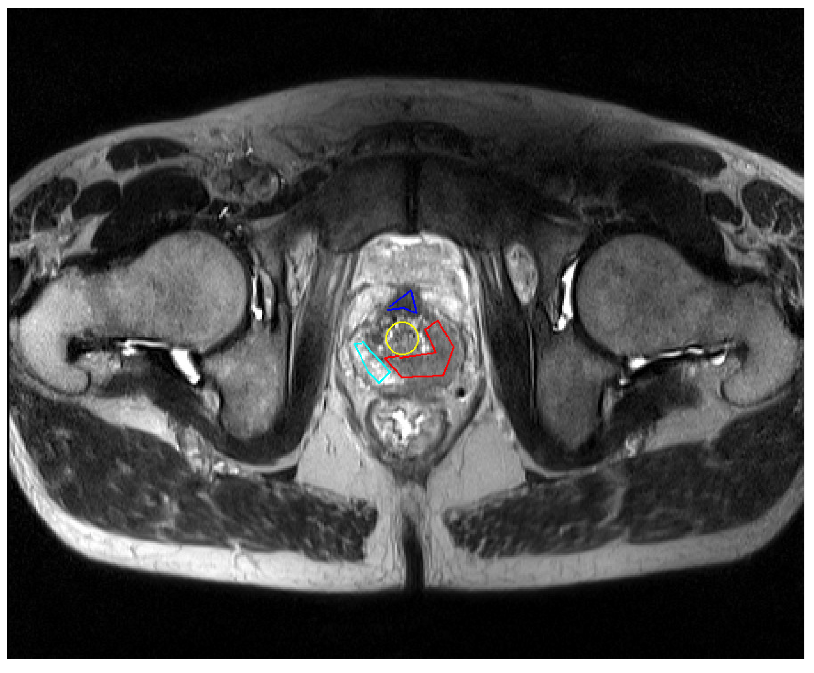
First, the user must load an image in DICOM format. For this application, the snake initialization is required; an example of the initial contours for a study is shown in
Figure 8. In the area of the GUI that corresponds to the initialization of the snake, the three first buttons are used for selecting the different zones of the prostate, whereas the fourth one gives the possibility of selecting a tumor.
Located below these buttons, there are two radio buttons, enabling to choose the shape of the initial contour, which can be circular or manual. The first option corresponds to an initial contour with a shape of a circle whose radius can be specified with the spin box located at the end of this area. The possible values are between 1 and 30 pixels. The manual input enables the user to enter a random polygon as initial contour. If selected, the user just has to make a click with the mouse in the vertices of the desired polygon. There are no limits for the amount of points, or the shape of the polygon.
The steps required to initialize the snake for any of the prostate areas are the following:
Select the type of contour to enter, circular or manual. In case of circular, enter also the radious.
Select an area: TZ, PZ, CZ or Tumour.
Create the initial contour for the snake in the left image. If it is a circle, the mouse cursor must be placed in the center of the area of interest, and click with the left button of the mouse. If manual contour has been chosen, the mouse must be placed in the point where the user wishes to start the contour and make click with the left button. Then move the cursor until the next point, make a left click and go to the next point. More than 2 points are required.
In manual mode, once the contour is finished, press the “Ok” button. If not, go to step 5.
A message box will appear informing if the contour has been correctly added or not.
The user can repeat the same procedure for all the zones, or just some of them. In order to differentiate the various selected areas, each initial contour will be drawn with a different color. There are no constraints about the type of contours to use. All the contours can be manual, all of them can be circles or they can be a combination of them.
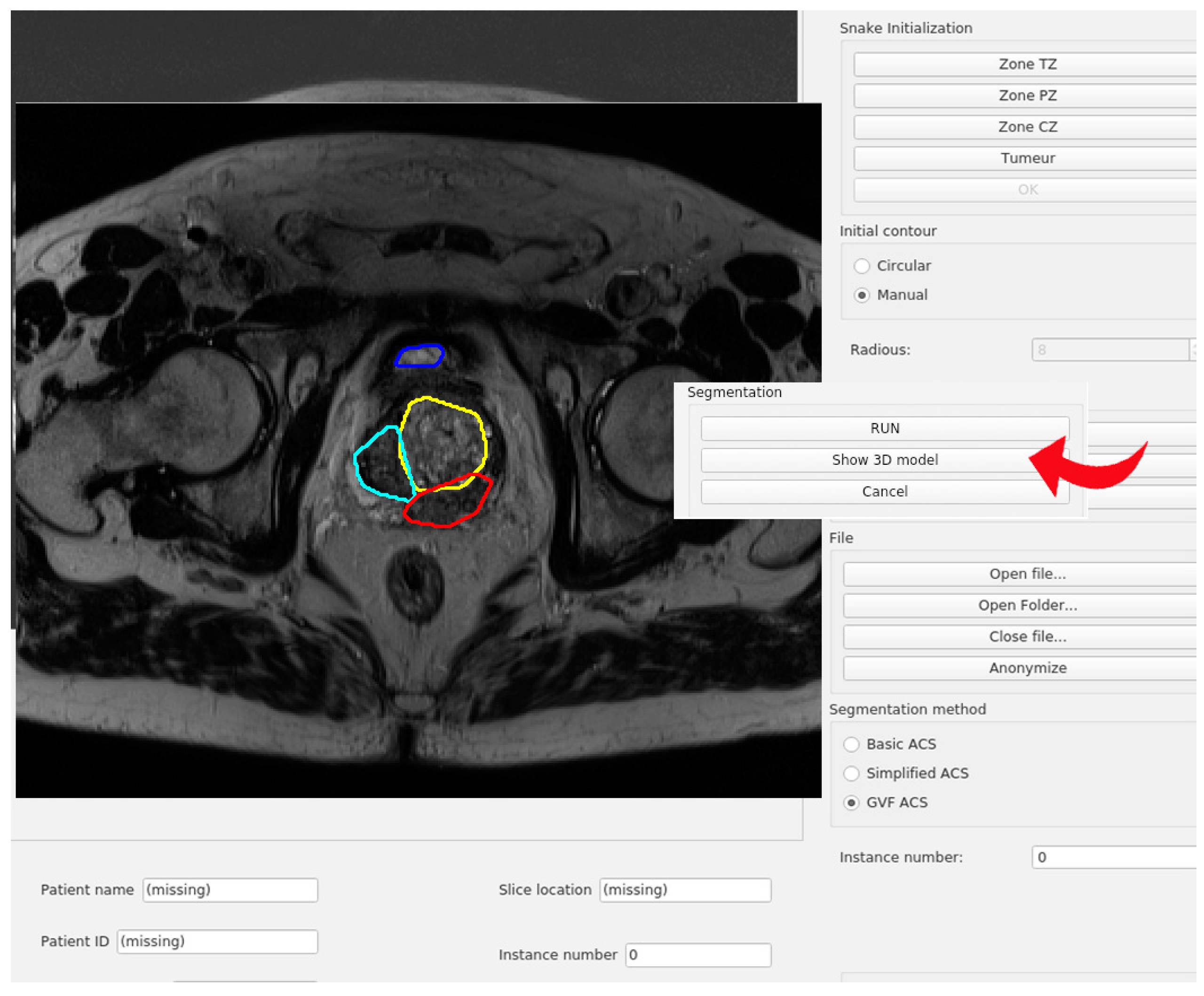
The following area of the control panel is used for triggering the segmentation. This section is depicted in
Figure 9. After an image has been loaded, at least one initial contour has been entered, then the segmentation process will start after pressing the
button. The segmentation method will be triggered as many times as initial contours have been entered, and they will be executed sequentially. During this process, the user can cancel the segmentation at any moment, pressing the
button. Once the algorithm had finished, the results will be shown in the right image. Additionally, the color code of the contours is the same for both, left and right images. For instance, the resulting contour of color blue in the right image has as initial contour the blue snake from the left image.
If some results have been produced, then a 3D representation of them can be visualized if the user presses the button
. This representation consists only of the resulting contours, replicated several times along the Z axis. It is an extra option for users to visualize the main structure of the segmentation in a 3D model. In fact, this option should be improved using better visualization techniques, but it is out of scope of this work for the moment. The amount of repetitions has been set to 50. The axis are represented in real scale, in mm, if the DICOM file contains the information about slice thickness and spatial resolution. If they are not provided, a pop up message will appear reporting the situation, and the X and Y axis will be presented in pixels, and the Z axis will have a size of 10 units. An example of this 3D representation of a result is shown in
Figure 10.
Regarding to file management tasks provided to this tool, users can open a DICOM formatted file or a folder that contains several DICOM formatted files. When the button is pressed, a pop up window will appear, and it will only allow the user to select a file, not folders. If a file is not in DICOM format, then the program will reject it, and it will not do further actions. If the user wants to open a folder, it should click the button, navigate until the folder it wants, and go into that folder. Without touching any file, users should click the button and the system will automatically search for files, and open only the DICOM formatted files. It is important to emphasize that the search system is not recursive. That means, if there are folders inside the selected one, and those folders contain DICOM files, the program will not open them. It will only open the files that are in the current directory.
As it can be seen in the graphical user interface, there are three types of algorithms:
Basic ACS,
Simplified ACS and
GVF ACS. The first and the second algorithms are based on [
12], but the second one does not follow the mathematical approach described in this previous work. On the other hand,
Basic ACS implements exactly what the paper states, as explained in
Section 2.3. Both algorithms have been included so that there is an example in the code of how to add a new algorithm to this code-base. Additionally, the
Simplified ACS performs a faster than
Basic ACS but with less accuracy. Nonetheless, in order to produce improvements to the original paper, the
Basic ACS was required.
Finally, considering that this application is focused on DICOM format and it can be used for radiologists and/or medical experts, it is important to maintain the private information of the patient. For this reason, an anonymization module is integrated in this tool. If the user wants to anonymize the opened file or files, it should click into the Anonymize button. If there is a file/files opened, a pop up window will be shown where the user must specify the destination folder of the anonymized files. The name of the output files will be the same as the source files, but the string will be appended to it. For instance, if the original file is called , the output file will be called . The fields that are anonymized are: Patient Name, Patient ID and the Patient Date of Birth. Those fields are not cleared, but changed by some default data: Patient Name is changed by NN, Patient ID is transformed to A00000000000, and the date of birth is changed to 01/01/1970.
We believe that the proposed tool can be beneficial for the research community as it enables to integrate various image management tools thoroughly discussed in previous sections, as well as the capability to segment prostate cancer lesions and other areas as mentioned in the introduction. Even though the application includes the option of segmenting four zones only (CZ, TZ, PZ and Tumor), nothing stops the users of trying to segment other areas of their interest (additional buttons can be appended into the GUI in order to select more areas, or the already existing buttons can be used to segment those areas). These features, as well as the capability to integrate new segmentation models seamlessly make it very appealing for research and teaching purposes in clinical settings. In the former case, it can help in speeding up the creation of datasets for machine learning applications. However, in our experience, doctors are reluctant to use fully automated annotation tools and prefer to use interactive semi-automated tools that enable them to verify and contrast the results with other specialists. In order to test the performance of the proposed tool, we performed one experiment to assess the quality of the segmentation algorithm implemented in this work, which will be detailed in the following section.
4. Discussion of the Segmentation Method Results
In this section, we present a deep analysis of the results of a single segmentation experiment performed using the implemented algorithms, namely the
Basic ACS,
Simplified ACS and
GVF ACS versions of the snake-based models. For all the cases, the initial contours used for all the zones are shown in
Figure 11.
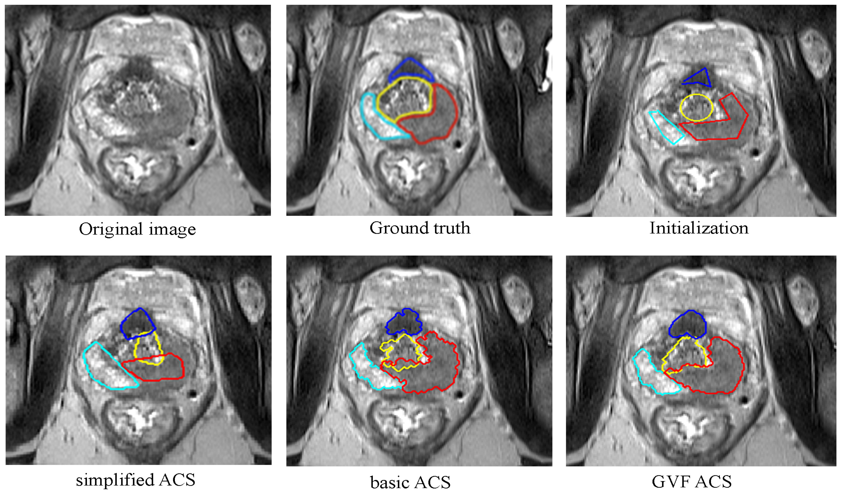
The results for all the algorithms and the ground truth for the selected image are shown in the
Figure 12.
From this experiment, it is possible to confirm what it has been said in previous sections. The Basic ACS algorithm performs relatively well when there is some gradient information between different areas. In this image, the cyan and the blue contours (corresponding to the PZ and CZ, respectively) are practically attached to the borders; the contour corresponding to the TZ (yellow contour) is almost perfect. Nonetheless, the tumour area invades the TZ area, since the intensities contrast between them is not enough in order to define a good edge.
For the case of
Simplified ACS, the results are not so satisfactory. This algorithm is uses simplifications of the formulas described in [
12]. It has been tested for heart’s left ventricle segmentation and it has a good performance in both, quality and speed, but for prostate segmentation, this is not true. Except for the TZ, all the results take part of the other zones, and only when the edge is too strong, the snake seems to be perfectly attached to it.
Finally, as it is expected, the Gradient Vector Flow implementation overcomes all the problems, and the curves are strongly attached to the borders of each zone. There is only a little overlapping between the tumour and the TZ.
Another point to observe is the smoothness of the results from Basic ACS and GVF ACS. None of them include either a shape prior or the smoothing factor. This allows the snake to evolve in any shape, which is desired in this case, since there is not a single prior that work for all the prostate zones. Additionally, for the same reason, a generic post-processing that increases the smoothness of the curves is not trivial to implement. This problem is visible mainly in the result given by the Basic ACS, where all the contours do not present smooth borders. Nonetheless, the GVF ACS generates a result that even without these factors, the outcomes are not so jagged. Once again, the addition of the Gradient Vector Flow component surpasses the results given by the Basic ACS.
It is worth mentioning that the initialization (in all the cases) requires to be inside of the object to produce valid results. Since a lot of objects are present in an MR image, a larger contour than the object will produce poor segmentation results. In order to reduce this effect, the image to be segmented is cropped to an square of 150x150 pixels around the center of the initialization contour before starting the segmentation process. As a consequence, not only the influence of other objects over the snake is reduced, but also it reduces the execution time, since less operations are required at each iteration of the algorithm.
In order to measure quantitatively the efficiency of the three model implementations, a contour evaluation of this test was performed. For this evaluation, the Hausdorff distance (HD) and Dice index (DI) metrics for the various segmentation results were compared with a ground truth provided by a specialist. The Hausdorff distance between two finite set of points A and B is defined as follows:
where
is the directed Hausdorff distance defined by:
where
is the Euclidean distance and
A and
B are the resulting contours of the segmentation.
In computer vision and image processing applications, the largest segmentation errors quantified using the Hausdorff Distance can be a good measure of the usefulness of the segmentation for the intended task. Intuitively, is the longest distance one has to travel from a point in one of the two sets to its closest point in the other set. In image segmentation, this metric is computed between boundaries of the estimated and the ground-truth segmentation, which consist of curves in 2D. We computed the Hausdorff distance between the generated segmentation and the ground truth. The methods with the lowest distance are considered to have yielded the best segmentation results.
Another popular metric for image segmentation tasks is based on the Dice coefficient, which is essentially a measure of overlapping between two samples and it is equivalent to the F1 score. This measure ranges from 0 to 1, where a Dice coefficient of 1 denotes perfect and complete overlap. This metric is calculated as:
In
Table 1, we summarize the results obtained from the performance analysis for the three segmentation methods, using the two above-mentioned metrics. This procedure has been done for each of the prostate’s gland zones, which corresponds to the examples of the annotations depicted on
Figure 12. The ground truth is used as a reference image to calculate all the measurements. First, according to the initialization image, a comparison of the results between
Simplified ACS,
Basic ACS and
GVF ACS is performed. It can easily be inferred from the table that the
Basic ACS yields more accurate segmentation results in all the prostate zones than the
Simplified ACS. Moreover, it can be seen that the
GVF ACS implementation improves the results in all the cases.
The geometry of the zone is considered the most difficult part of the prostate MR image because it is difficult sometimes to demarcate the edges of this area, given that it is surrounded by the other zones; for this reason, it is important to do a good initialization. The results for the are good in all the cases, especially when GVF is used. Moreover, the results on the area are good for all the algorithms considered in this study. Finally, the results for the tumor area indicate that the best segmentation is obtained using GVF ACS methods.
Finally, in order to assess the performance of the various studied segmentation methods, a time analysis has been performed. As in
Table 1, the analysis has been divided by zones and by algorithm. Then, the execution time of the segmentation algorithm has been assessed for each zone, using the same initialization as in
Figure 11. For this test, a computer with a microprocessor i7-8650U @ 1.90 GHz, 16 gb of RAM and running Linux 4.15.0-64 has been used. The execution times are depicted in
Table 2. All the measurements has been done in milliseconds. Both
Simplified ACS and
Basic ACS run at maximum 200 iterations, and the
GVF ACS runs at maximum 80 iterations. Both
Table 1 and
Table 2 confirm what it has been said about the
Simplified ACS algorithm. It is the least accurate, but it runs faster than the other ones. On the other hand, even though the
GVF ACS runs less iterations than the
Basic ACS, their running time are similar. This is due to the
GVF ACS algorithm computes the same code, plus the additional ones in order to get the Gradient Vector Flow contribution. Nonetheless, for this work, this execution time could have been reduced if the equations related to the shape prior and the smoothness would have been removed. Only the weights have been set to zero for those priors. This code has not been erased so that other developers can prove other parameters values, and try to find other combination of weights to make this program work with either, other image modalities, or other organs to be studied.
These results show that a good segmentation can be obtained in a reasonably time, which is important for both clinical and machine learning applications. As it is expected, one result is not representative of the quality of these algorithms. An analysis of a larger population must be done in order to have a real measure of quantitative error of our implementations. The work we introduced here is to present the tool, the algorithms implemented and how to use them. As future work, we plan to perform a more comprehensive study encompassing other methods known to have good results to contrast results as well as other regions of interest within the prostate. This will enable us to assess the validity of the proposed segmentation approach in other setting, and to get feedback from a larger pool of specialists. Other avenues of research pertain the validation of the proposed tool, as well as of the segmentation algorithm in a larger pool o prostate MRI images, as well as with a wider number of clinicians. We also plan to integrate other segmentation methods into the proposed GUI tool to carry out a more comprehensive quantitative comparison and to investigate its diagnostic differentiation with other prostate diseases such as BPH, chronic or acute prostatitis.
5. Conclusions
In this paper we described the implementation of a snake-based segmentation algorithm, based on an Active Contours Models (ACM), which has been integrated into a GUI based application. We focused our research in a method originally conceived for segmenting the shape of the heart’s left ventricle. A modification of this specific prior has yielded very good results in the context of prostate cancer segmentation: the snake models tries to evolve and to adjust to the boundaries of the proposed zones. The problem with this implementation is that the performance of this previous model highly depends on the quality of the input image, as it uses the pixel intensities and the edges of the object in order to determine the correct curve evolution. As it can be expected, if the boundaries are not well defined, or if the intensities of different sections have similar values, then either the model will not be able to assess the difference, preventing the algorithm of evolving, or it will cause the snake to overlap with other elements in the image. This scenario can be observed in
Figure 12, where the red contour overlaps with the area that corresponds to the TZ.
Furthermore, in order to get that segmentation, several shapes for the initial contours had been tested to obtain the best results, which might be very different from one run of the algorithm to another. This entails that the implemented snake-based algorithms are very sensitive to the initialization conditions. This type of problems have fostered researches in image analysis and computer vision to find novel ways of constraining the shape of the force that pushes the objects’ boundaries in the right direction. Doing so, the segmentation algorithm becomes robust against to initialization conditions and less sensitive to the quality of the image.
Regarding the performance of both implementations, the
Simplified ACS and
Basic ACS, their behaviour are not the same. Since
Basic ACS includes all the weights and all the functions described by the original document, the boundaries of the final segmentation tends to be closer to the real boundaries of the object to segment than in the case of
Simplified ACS. Nonetheless, both of them fail in the task of finding the boundaries when the image intensities between two contiguous areas are not noticeably different, like in the case of the tumor and the central zone in
Figure 12. This problem has been partially overcame when using the Gradient Vector Flow external force.
Further improvements to this algorithm will thus be directed towards implementing other types of Gradient Vector Flow energy optimization algorithms, or exploring how to include shape priors for each zone of the prostate separately. These modifications would help to create a segmentation that does not go too far from where the real object is. Additionally, no pre-processing nor post-processing functions have been included. Adding pre-processing operations might help to remove the noise that addresses the snake towards the wrong directions, and post-processing of the resulting contour will help to make it smoother, and closer to the real boundaries of the object.
Moreover, since the DICOM files can contain different image modalities, and each modality has its particularities, a profiles section can be added to the program. Each profile will contain a set of parameters (priors weights, GVF weight, regularization constants, and iterations) specific for each algorithm. These profiles will be chosen in a way that they will produce the best segmentation results for the selected image modality, increasing the scope of application of the program.
Other avenues of research pertain the validation of the proposed tool, as well as of the segmentation algorithm in a larger pool o prostate MRI images, as well as with a wider number of clinicians. We also plan to integrate other segmentation methods into the proposed GUI tool to carry out a more comprehensive quantitative comparison and to investigate its diagnostic differentiation with other prostate diseases such as BPH, chronic or acute prostatitis.
