Article

Urban Ecosystem Services (UES) Assessment within a 3D Virtual Environment: A Methodological Approach for the Larger Urban Zones (LUZ) of Naples, Italy

Department of Architecture (DiARC), University of Naples Federico II, 80138 Napoli, Italy
*
Author to whom correspondence should be addressed.
Appl. Sci. 2020, 10(18), 6205; https://doi.org/10.3390/app10186205
Submission received: 18 June 2020 / Revised: 28 August 2020 / Accepted: 4 September 2020 / Published: 7 September 2020
(This article belongs to the Special Issue Big Data in Geocomputation for the Built Environment)

Abstract

:
The complexity of the urban spatial configuration, which affects human wellbeing and landscape functioning, necessitates data acquisition and three-dimensional (3D) visualisation to support effective decision-making processes. One of the main challenges in sustainability research is to conceive spatial models adapting to changes in scale and recalibrate the related indicators, depending on scale and data availability. From this perspective, the inclusion of the third dimension in the Urban Ecosystem Services (UES) identification and assessment can enhance the detail in which urban structure–function relationships can be studied. Moreover, improving the modelling and visualisation of 3D UES indicators can aid decision-makers in localising, analysing, assessing, and managing urban development strategies. The main goal of the proposed framework is concerned with evaluating, planning, and monitoring UES within a 3D virtual environment, in order to improve the visualisation of spatial relationships among services and to support site-specific planning choices.

1. Introduction

The new EU Biodiversity Strategy for 2030, “Bringing nature back into our lives”, has identified a comprehensive, systemic, and ambitious long-term plan for protecting nature and reversing the degradation of ecosystems, driving the recovery from the urban crisis, and helping to strengthen the resilience of cities against future crises. These recommendations aim to halt the loss of biodiversity and Ecosystem Services (ES) by 2020 and enable transformative change. These challenges require new approaches and tools that support the aim to make ES mapping, monitoring, and assessment mandatory within European countries [1]. The last report of the OECD estimated that 125–140 trillion US dollars per year of benefits are provided by ES at the global scale, while the cost of global policy inaction on biodiversity loss per year between 1997 and 2011 was 4–20 trillion US dollars, underlining the need to identify suitable tools to assess risks and opportunities related to ES, as well as their environmental impacts and dependencies, with specific attention at the local-site level [2].
As the definition of ES is context-dependent, the concept identifies a boundary object for sustainability—namely, an idea embedding different points of view—which preserves a sense of continuity, engages different disciplines and non-scientists in shaping and achieving societal goals, and is instrumental in facilitating, implementing, and assessing transformative processes for more sustainable human–nature relations [3,4,5,6,7,8,9].
According to Costanza [10], sustainability valuation for ES requires an integrated and whole-system approach at appropriate spatial and temporal scales that is able to interpret the complexity of interactions related to ES production.
Indeed, the Millennium Ecosystem Assessment (MEA) has adopted a definition that includes the spatial pattern and the social dimension as results of human–nature interactions in the provision of services and benefits for human beings [11]. Therefore, attention to the specific dimension of the context, the scale of change and urban characteristics, and the level of perceived influence are some of the most significant issues that need to be considered when identifying and assessing ES [12].
Nevertheless, when dealing with the urban dimension—as the place in which the built environment prevails over natural features and the population density is high—the specification of “Urban Ecosystem Services” (UES) needs to consider the actual role of ES within the city context [13,14,15,16].
At the same time, some authors have interpreted the concept of UES according to the different relevance attributed to the definition of “urban ecosystem services” or “urban ecosystem services” [17]. The first concept is related to ecosystem services as analogues of natural and semi-natural ecosystems within urban boundaries; it is prevalent in the UES literature and deals with the natural and semi-natural spaces within cities [18].
The second definition expresses a much broader term, including the former group as well as urban settings in a city, covering the full range of services produced by humans, including housing, transport, education, entertainment, or medical care, with attention to any service relating to urban areas useful for urban dwellers [19].
Moreover, Tan et al. [17] pointed out that the definition of UES and its application are context-dependent and able to express the interpretations of relationships that link UES to natural and human-derived capital, exploring how a broader interpretation of UES might advance its implementations. In this context, UES can be considered as a pattern of multidimensional services locally produced in cities to guarantee human wellbeing in both tangible and intangible ways [17,20], which is able to support policies and programs for planning and managing cities.
The city, as a complex socio-ecological system [5,21], needs suitable methods and tools that aim to:
  • Analyse the spatial configuration and linked ecological processes [22];
  • Preserve natural, social, built, and human capitals [23];
  • Evaluate UES at different scales, through multi-scale approaches [24];
  • Measure sustainability and resilience through spatially explicit assessments [25].
In this perspective, 3D data acquisition and visualisation allows for better investigating the spatial configuration of cities, which affects human wellbeing and landscape functioning [26], as well as aiding in the identification of enabling conditions for transformative changes. The communication of social–ecological flows within the analytical procedures of urban planning can be improved, and explicit UES trade-offs can be detected to spark sustainable decision-making processes [27]. At the same time, understanding and safeguarding the supply of UES that derive from the four capitals allow for tackling the challenges of sustainability at both ecological and administrative scales—for example, releasing urban policies in harmony with Urban Metabolism (UM) principles [28].
Within UES and UM frameworks, studying metabolic flows at regional and urban scales in a 3D virtual Geographic Information System (GIS) environment can improve policy-making, addressing the preservation of capitals within multidisciplinary sciences for several reasons. First, Digital Terrain Models (DTMs) and 3D ground visualisation can enrich flooding risk analysis within watershed modelling [29]. Secondly, cross-cutting data on climatic zones, land-use, and building heights better inform decision-makers about spatial adaptive strategies for resilient cities [30]. Moreover, 3D UES mapping within multi-group decision-making could facilitate collaborative scenario generation for the enhancement of the multi-functionality and the ES supply, whenever those services are scarce or entirely lacking.
For the last ten years, mapping two-dimensional (2D) UES has improved data communication for more informed decision-making [31], better interactions among local communities and cultural landscape values [32], integrating ES into Strategic Environmental Assessments (SEA) for sustainable urban planning [33], and generating awareness of the most valued and used locations, in terms of services and their benefits [34,35]. Nevertheless, some authors have remarked on the following limitations when referring to 2D UES mapping:
The unsuitability of representing multiple services at the same location within a unique map and the loss of aggregated information regarding the change in service bundles through time and space [26];
The impossibility of simultaneously visualising UES trade-offs [36] (i.e., those linked to the imbalance of a spatial policy maximising economic capital to the detriment of ecological services);
The difficulty of representing spatial relationships among z-elevation values and specific UES, such as the relationships useful for quantifying biodiversity loss within ecological modelling studies [37] or the spatial correlations among building z-values and other Urban Heat Island (UHI) indicators [38];
The lack of combining visual and non-visual information for the participatory assessment of scenarios in workshops [39].
Therefore, the inclusion of the third dimension into UES assessment could address and solve some of the limitations mentioned above, highlighting the details of urban structure–function relationships. Furthermore, multi-scale assessment aids in the understanding of regional planning outcomes in terms of social, ecological, and economic dynamics, by comparing processes, features, and the interests of stakeholders operating at different scales [40].
Moreover, the integration of GIS and Multi-Criteria Decision Analysis (MCDA) allows for implementing spatially explicit assessments [41], which are crucial for deeply analysing social–ecological city systems and their relationships. Furthermore, matching multi-scale elements on homogenous cells of analysis [42], referred to as Minimum Mapping Units (MMU) [43], can provide a significant step forward within the “integrated valuation” methodologies [10,44,45,46,47,48,49], as this contribution aims to outline.
Despite the potential of 3D applications in many scientific fields [50,51], a significant gap in knowledge within the ES literature regarding the development of 3D city modelling combined with UES assessment is evident. In particular, studies that take into account the volume of urban services and building heights are lacking. Considering these knowledge gaps, two main questions arise, which motivated this paper:
How can 3D GIS-based modelling better transfer relevant information to inform decision-makers about the localisation, assessment, and management of UES?
What is the role of 3D modelling and virtual decisional environments concerning the communication, democratisation, and negotiation of UES?
In this framework, one of the main issues in sustainability research is to conceive models that are capable of adapting to changes in scale and recalibrating the selected indicators, depending on the degree of detail and data availability. The evolving definition of scale is a fundamental part of a multi-scale approach [52], where scale emerges as a dynamic concept that differs, at any one place and moment, depending on whether it is being applied to a problem definition, to an empirical observation, to an analysis, or to an anticipated action [12], reflecting real-world dynamics and ranges of variability.
Another issue is related to the opportunity to disseminate the UES application, overcoming the different barriers to the effective implementation of ES assessments in management and policy, one of which is particularly relevant and is related to bridging the science and policy gap and building trust among scientists and the broader community of stakeholders: improving the inclusiveness of assessments and overcoming the limits and bias that reflect the interests and expertise of a select group of people [25,53,54,55]. The opportunity to visualize, through 3D modelling, the characteristics of the UES and the effects of transformations allows us to involve not only different types of experts but also citizens and non-experts in the assessment, who are the people who actually receive the benefits and who have an in-depth understanding of their perceptions and values [53,54,56,57,58,59,60].
This paper aims to test a methodological approach that relates 3D urban modelling and visualisation to the UES assessment, considering the Larger Urban Zones (LUZ) of Naples (in the South of Italy) as a case study and structuring a Spatial Decision-Making Support System (SDMSS) that integrates GIS and MCDA.
The rest of the paper is structured as follows: Section 2 presents the materials and methods, describing the different phases of the proposed methodological approach. Section 3 introduces the case study, through the data, indicators, and multi-criteria methods used to implement the 3D UES approach. Section 4 provides the results. Section 5 explains the discussion, and Section 6 presents our conclusions about the development of the methodology proposed for city planning and decision-making.

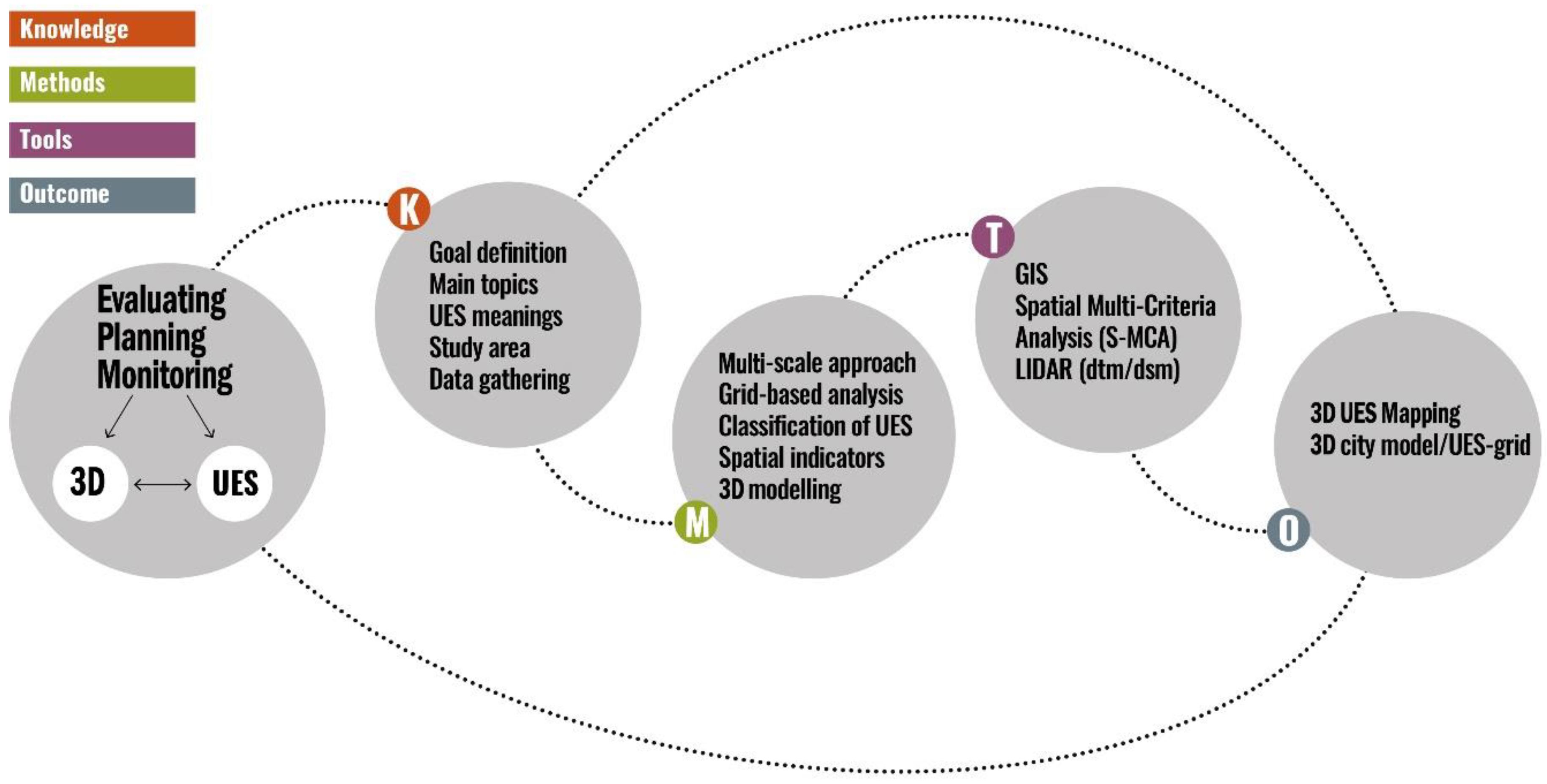
2. Materials and Methods

The methodological framework (Figure 1) identifies four inter-related phases: knowledge (K), methods (M), tools (T), and outcome (O).
The main goal of the proposed approach concerns UES evaluation, planning, and monitoring within a 3D virtual environment, in order to improve the visualisation of the spatial relationships among the service allocation and the urban fabric density. The framework of a Spatial Decision-Making Support System (SDMSS), where GIS tools, Multi-Criteria Decision Analysis (MCDA) methods, and Light Detection and Ranging (LiDAR) technology work together and support one another, represents the context of our experimentation.
The first phase seeks to identify the main topics concerning the recognition of UES, their characteristics, and their spatial benefits in a selected focus area. As the preparatory step of the proposed approach involves data gathering and processing, both authoritative sources and Volunteered Geographic Information (VGI) were considered useful for enhancing the knowledge related to the urban context. A specific data set was structured and elaborated through GIS tools, within the GIS environment, which is able to identify and classify the different types of information and data gathered [61].
The second phase concerns the application of a multi-scale approach and a grid-based analysis to normalise the data on a standard surface. A grid of 500 × 500 m per cell, which extends over the boundaries of the selected focus area, was assumed as the MMU, as it better includes the natural and built features in the examined environment. The use of a regular-shaped (i.e., a rectangular or square) grid is generally preferred in environmental studies, as the orthogonal co-ordinate system and the raster format are the most common parameters in the release of spatial data [62]. The multi-scale approach allows for assessing spatial indicators—referred to proxies for detecting UES features and dynamics—through the mapping of geographical entities that produce benefits [12,63]. This approach requires choosing a homogeneous statistical surface on which indicators with different sources, formats, attributes, and spatial resolutions can be processed, analysed, and compared [64]. In this phase, the selected spatial indicators are represented by 3D modelling.
The third phase aims to choose suitable MCDA methods to integrate with LiDAR technology. The spatial MCDA allows for computing the values of the normalised indicators representing the performance of each cell, in terms of UES supply. LiDAR technology was adopted to combine the UES values with the 3D city visualisation, as it has been broadly applied in 3D urban modelling [65,66].
The fourth phase allows for producing a twofold outcome. The first outcome shows the 3D data mapping of three UES categories, while the subsequent outcome overlays the UES grid with the 3D city model to enhance the spatial results and to permit the comparison of UES indicators per cell.
The expected results address an application of the proposed multidisciplinary research, combining and involving different academic disciplines or professional specialisations (e.g., urban and landscape planning, forestry, agriculture, and UM disciplines) to solve some critical issues. To provide some examples, it can facilitate:
The resolution of spatial problems that involve the allocation of resources/services in a high-density context;
The 3D UES visualisation of indicator values at multiple scales and locations;
The spatial assessment of multiple scenarios related to stakeholder preferences within a virtual decision-making environment;
The development of a dynamic web-GIS platform, through which planning demands and “integrated evaluation” tools can be matched with one another.
In the proposed methodological process, a key role is assumed for the data that can be used for the structuring of the 3D model. The source of the data and their typology are analysed in Section 2.1, providing details about the sources useful for 3D UES modelling, as well as the implemented technology and tools.

2.1. Technology and Tools for 3D Modelling

Authoritative databases and Volunteered Geographic Information (VGI) systems-i.e., OpenStreetMap (OSM), Flickr, and Wikiloc - allow for the collection of available data relating to the 3D features of the urban system. In particular, VGI enriches knowledge at an urban scale through user-generated content (i.e., buildings, infrastructures, facilities, and points of interest). Planning and managing UES within an urban decision-making environment require upgraded tools to monitor the state of services by identifying potential and critical levels, prioritising actions, and geo-locating optimal solutions rapidly and effectively.
Notwithstanding some limitations, by dealing with the incompleteness over broad zones and geometric heterogeneity, VGI frequently provides more accurate data than authoritative sources [67]. Many authors, indeed, have remarked upon the completeness and semantic accuracy of the OSM data set, through its comparison with authoritative databases [68,69,70]. One of the main advantages of using these types of data (e.g., those derived from Flickr, Panoramio, or Instagram) may concern the coverage of zones with scarce or limited availability of official information, due to financial and governmental restrictions [71].
Regarding the control system for user contributions, statistical sampling methods that allocate points in a grid system have been used to limit the uncertainty, to acknowledge locations in which more in-depth data are needed, and to understand which type of information has been requested [72,73].
Furthermore, LiDAR technology provides relevant 3D information to improve the knowledge regarding the built and natural capitals of a city, in terms of accurate elevation-based values for buildings, vegetation, and other surfaces, at one metre-to-ground resolution.
According to Shiode [74], LiDAR is one of the data-acquiring methods commonly used for 3D urban modelling with geospatial technology. It employs laser rays to measure the position of a point in space, by recording first-pulse and last-pulse return rays, depending on the different properties of the absorption and reflection of laser beams of the detected object [74,75].
Digital Terrain Models (DTMs) and Digital Surface Models (DSMs) are the primary outcomes that the system produces from object heights. A DTM is a mathematical grid model of the Earth’s surface, in which each pixel has a unique elevation value, whereas a DSM is a mathematical grid model that includes the elevation values of off-ground objects (e.g., buildings and vegetation) [76]. Finally, the object heights can be found by subtracting the DSM from the DTM, combining the opportunities of the two tools and processing the elevation data necessary for spatial analyses.

3. Quantification, Assessment, and 3D Visualisation of UES in Naples
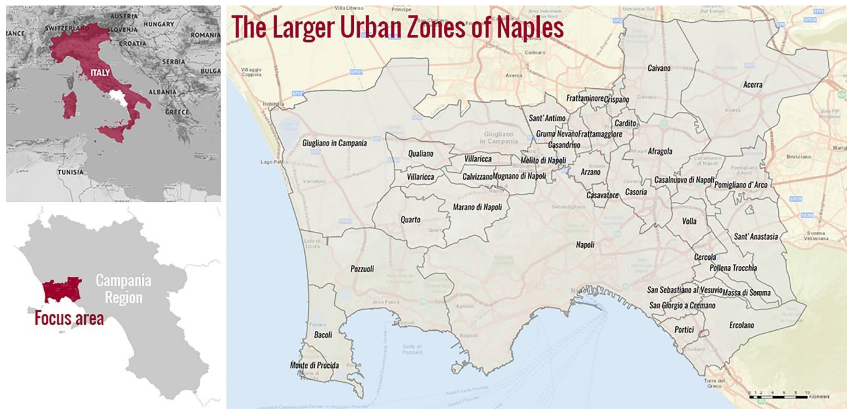
The selected case study aimed to test the methodology of the 3D UES modelling. The purpose was to evaluate the status of services within the administrative boundaries of Naples city (Italy) and its surroundings, combining GIS tools and the spatial multi-criteria extension of the Analytic Hierarchy Process (AHP) method [77]. This section of the contribution aims to expand upon the MCDA results presented by Mele and Poli [78].

3.1. Case Study

The focus area extends over the Larger Urban Zones (LUZ-) of Naples, as conceived and mapped by the European Environment Agency (EEA) with the “Urban Atlas” project [79]. The focus area in Figure 2 is approximately 560 sq km, including Naples city with its 960,000 inhabitants, 14 satellite municipalities connected to the urban core directly, and 21 municipalities affecting the city in terms of economic, social, and environmental pressures.
The Naples LUZ were chosen as a case study, as they represent a typical urban context in which neighbouring geographical regions have very different morphologies, with an uneven spatial organisation of the districts and scattered high-density zones. The peculiarities of an urban landscape featuring all of these components are suitable for being represented spatially by a 3D GIS environment. In this way, the UES spatial distribution can help to contextualise planning actions appropriately, as well as helping in the observation of the statuses of Regulation, Carrier, and Information services and the evaluation of their changes in space and time. Another reason for choosing this area relates to its data availability. OSM and Urban Atlas—which are the most relevant data sources for this application—release regular updates for the focus area.

3.2. Classification of UES

Urban Ecosystem Services have been addressed by some relevant initiatives, such as the Millennium Ecosystem Assessment [80] and The Economics of Ecosystems and Biodiversity [81].
A review of the ES approach [82,83] has shown a wide range of ecosystem service classifications considering the typology of services and the meanings of the main terms related to “process”, “function”, “service”, and “benefits”. Some relevant classifications [11,26,81,84] have defined services as those that can affect human wellbeing, either directly or indirectly. However, there are also other interpretations, which are conflicting in some cases. There is a lack of consensus related to the meaning of the term “function”. Some authors [84,85] have defined “function” as the expression of an “ecosystem process”; for other authors, instead, this concept relates to the capacity of ecosystems to provide goods and services [26,86,87], underlining an anthropocentric point of view and considering that a function becomes a service when humans enjoy it. The European Environment Agency (EEA) proposed a Common International Classification of Ecosystem Services (CICES) [88,89] by using ES typologies refined to reflect the key emerging issues highlighted in the most recent research literature. The CICES defined an explicit hierarchical structure that includes the three familiar ES categories (Provisioning, Regulation and Maintenance, and Cultural), where the major “Sections” are organised into “Divisions”, “Groups”, and “Classes” [89,90], serving as a suitable tool for integrating ES into analytical models supporting landscape and city planning.
Luederitz et al. [18] and Antognelli and Vizzari [19], starting from the above reflections, have underlined the role of the urban dimension, with specific attention to UES and their classification, with the purpose of providing a framework for conceptualising and managing human–environmental interactions within the broader context of sustainability [91].
Indeed, Luederitz et al. [18] considered that UES reinforce the idea that ES can be produced in urban areas to support human wellbeing in both tangible and intangible ways, and that UES can be considered as a social tool for bringing together different stakeholders to foster community-driven and government-led planning for urban sustainability implementation [92].
According to Tan et al. [17], the classification of UES considers four main types of services—Provisioning, Regulation, Supporting, and Cultural—where the term “service” is related to the aspects of the ecosystems used (either actively or passively) to support human wellbeing and characterised by two components identified as “structures” and “processes”, expressing relationship systems in cities. In particular, structures consider the social, ecological, and technological components of cities, while processes are related to the flows of materials, energy, and information occurring between and within these components. Therefore, UES derive from the stocks and flows of natural capital, but their realisation is also connected to other forms of capital, the so-called “human-derived capital” [93,94], which includes “produced capital”, “human capital”, “social capital”, “cultural capital”, and “financial capital” [17,95,96].
According to the above reflections, the classification of UES for the selected study area derives from the categorisation proposed by Vallés-Planells et al. [97], including the considerations of Gómez-Baggethun and Barton [13], as it provides more flexibility regarding the selection of a broader range of functions, which are able to describe the primary services related to the urban dimension. Indeed, the UES functions have been explained by de Groot [87]:
Regulation, considering a group of functions related to the capacity of natural and semi-natural ecosystems to regulate essential ecological processes and life support systems through biogeochemical cycles and other biosphere processes. Regulation functions maintain a “healthy” ecosystem at different scale levels and provide the necessary pre-conditions for all other functions.
Carrier, including a group of functions related to different human activities (e.g., cultivation, habitation, and transportation) that require space and a suitable substrate (soil) or medium (water or air) to support the associated infrastructure, involving the permanent conversion of the original ecosystem.
Information, selecting essential “reference functions” that contribute to the maintenance of human health by providing opportunities for reflection, spiritual enrichment, cognitive development, recreation, and aesthetic experience.
Assuming the classification of functions suggested by de Groot [87], Table 1 shows the selection of indicators in six levels, identifying three functions of UES, the tier as the specification of the function, the units of measure, the type of geometric entity, the distance threshold (DT) in metres, and the data sources.
The geographical data were processed using multi-criteria procedures to provide indicators as proxies for UES status detection. The following list specifically explains each tier of the database that was gathered for the focus area, amounting to 21 tiers of geographical data with physical information.
Within the category of Regulation functions, the followings five tiers were processed:
Environmental protection area includes the surface per cell of Italian communitarian interest sites (SIC) and special protection zones (ZPS). These areas provide a relevant contribution to the maintenance/conservation of regulation services.
Waterbody shows the surface per cell of the sea, lakes, fish ponds (natural or artificial), and rivers. For specific locations, this indicator is a disservice, as the quality of water in proximity to urban centres is frequently compromised by pollution. Nevertheless, this contribution does not provide detailed data about this phenomenon.
Forest includes both protected and non-protected areas that provide a positive contribution to urban ecosystems in terms of biological exchanges, air quality, raw materials, and green footprints.
Land without current use refers to the abandoned areas that, if correctly managed, can improve the regulation service maintenance/conservation.
Waterway includes streams, drains, docks, and canals and was obtained by computing the values of the distance between the cell and the nearest waterway.
The following nine tiers belong to the Carrier functions category:
Railway shows the network of transportation by computing the values of the distance between the cell and railway tracks.
Roads contains the network of roads by computing the values of the distance between the cell and roads.
Airport shows the surfaces on which airports are allocated and the buffer of influence for the surrounding areas. Although airports are crucial for long-distance connections, they have a negative impact, in terms of noise and environmental disturbance, on ecosystems.
Port shows the surface of the coast addressed to port functions and the buffer of influence for the surrounding areas, in terms of noise, pollution, transportation of people and wares, and proximity to boarding points.
Bus/underground stop identifies the location of bus or metro stops, visualising the most accessible zones of the focus area.
Mineral extraction site shows the areas in which raw materials are extracted for the construction sector.
Habitation density shows an institutional data set provided by the EEA with information about housing density.
Waste disposal localises the waste disposals that gather waste from the study area.
Tourism facility identifies the highest concentration of the touristic facility points (e.g., hotels, B&Bs, and guesthouses).
Finally, the last six tiers belong to the Information functions category:
Cultural site highlights cultural heritage by identifying the number of cultural sites.
Place of worship shows the location of worship places, which are related to landscape spiritual values.
Sport and leisure contains sport and leisure surfaces, which are very important as they contribute to the regulation and cultural functions of the landscape.
Green urban area refers to green areas, which are very important in contributing to regulation and cultural functions.
Attraction place represents the places of attraction that polarise the flows of tourists and citizens (e.g., theatres, cinema, and observatories).
Attractive landscape feature represents an excerpt of a point pattern, based on a code that determines the places most photographed by citizens and tourists in the focus area. It simulates landscape attractiveness, as perceived by citizens or tourists. A perceptual investigation about the relationship between aesthetic value and landscape features would require surveys, which the authors have not provided in this contribution.
In the same manner as the data resolution and the MMU, the choice of DT influences the final results of the spatial evaluation. It must follow criteria matching the main objectives of the decision-making process. Indeed, environmental studies are affected by the urban configuration [98], which includes the distances and the interactions among elements in terms of effect decay, mostly when dealing with ES approaches.

3.3. Multi-Criteria Decision Analysis through the Spatial AHP Method

The aggregation rule of the spatial AHP method, implemented into the Multi-Criteria Analytical Scoring Tool (MASCOT) software [99], allowed us to produce a normalised index of UES per cell, using pairwise-compared indicators and the Euclidean distance method, referring to the DTM. The enhancement offered by the tool consists of the two-fold processing of the cell-by-cell weighted sum and the Euclidean distance among spatial elements. The number of objects within the DTM and their weighted sum provide the overall UES score per cell. Finally, UES indicator values can be standardised within the range of 0–1 using the Min–Max formula (1):
I i , k = a i k m i n i   { a i k }   m a x i   { a i k } m i n i   { a i k }
where a i k is the indicator value per cell and I i k is the normalized indicator.
The four operational steps for performing the spatial MCDA in the MASCOT software are as follows:
  • Bundling tiers in three thematic groups, referring to the Regulation, Carrier, and Information macro-categories;
  • Choosing the DT per criterion/tier (the DT determines the maximum weight for a cell touched by a tier; the weight decreases linearly, down to zero at the boundaries of the setting distance);
  • Weighting tiers through AHP pairwise comparisons at three levels (in this application, the Equal Weights method was used);
  • Scoring tiers with the weighted sum, in order to derive the overall results for each macro-category.
In particular, the weighting phase was performed by the attribution of judgments—with the 9-point “Saaty semantic scale”—at hierarchical levels referring to three bundles of pairwise comparison matrices. At the “macro-category” level, a matrix (3 × 3) was filled. The “categories” level includes three square matrices:
A matrix (5 × 5) for tiers within the Regulation Services “macro-category”;
A matrix (9 × 9) for tiers within the Carrier Services “macro-category”;
A matrix (6 × 6) for tiers within the Information Services “macro-category”.
At the last level, the “sub-categories” include fine-grained information related to some elements of the top categories. The “sub-categories” level contains:
A matrix (2 × 2) within the “Environmental protection area” category, which includes SIC and ZPS as polygonal items;
A matrix (4 × 4) within the “Waterway” category, which includes streams, drains, docks, and canals as polygonal items;
A matrix (14 × 14) within the “Railway” category, which includes yards, turntables, trams, subways, stations, rails, platforms, funiculars, monorails, narrow-gauge lines, abandoned lines, construction lines, disused lines, and light-rails as linear items;
A matrix (10 × 10) within the “Roads” category, which includes bridleways, cycleways, footways, motorways, pedestrian ways, pathways, steps, secondary roads, trunks, and tracks as linear items;
A matrix (2 × 2) within the “Bus/underground stop” category;
A matrix (4 × 4) within the “Tourism facility” category, which includes hotels, hostels, guest-houses, and campsites as point items;
A matrix (4 × 4) within the “Attraction place” category, which includes theatres, cinemas, and observatories as point items.
The AHP procedures allow for calculating weights, through formulas (2) and (3) [77,99]:
W i = M i K = 1 N M k ,
M i = j = i N A i j N
where Wi is the weight of the ith criterion and Aij represents the pairwise comparison matrices. The scoring cell derives from the multiplication of weights at each hierarchical level, while the weighted sum of each contribution determines the overall UES score per cell.

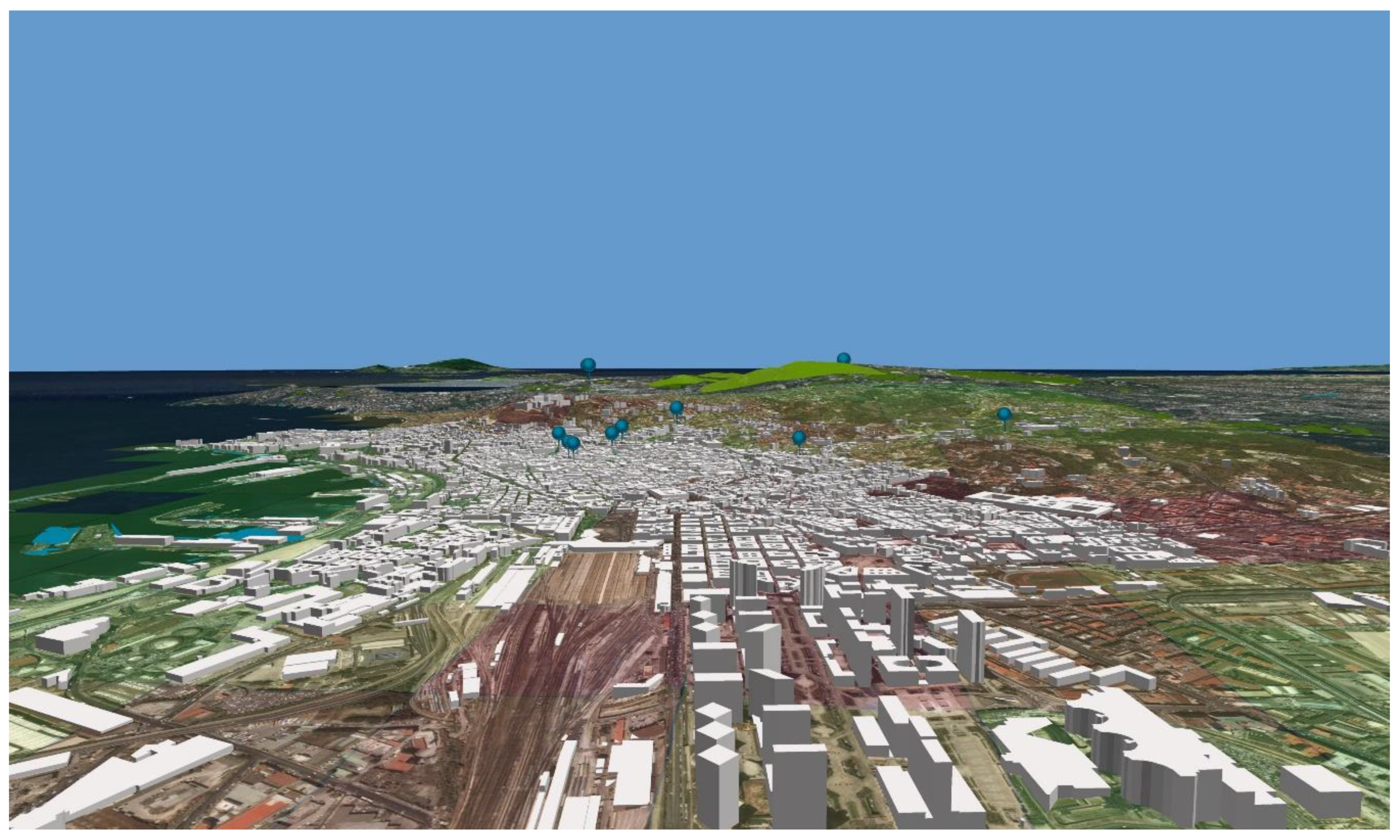
3.4. Operational Steps for 3D Modelling

Three steps are used to visualise the 3D UES mapping. First, the geographic entities that represent the UES must be selected and georeferenced, as shown in Figure 3A; then, the application of the spatial AHP provides the standardised indicator values per cell on the geodetic grid, as shown in Figure 3B. Finally, 3D histograms, assigning the normalised indicator values to the cell z-values, show the spatial distribution of UES for the Naples LUZ. In particular, the ArcGlobe software (within the ArcGIS 10.3 platform) allowed us to visualise the last step, as shown in Figure 3C.
Afterwards, the 3D city model allows for a better understanding of the existing relationships between urban districts and the status of UES.
The elevation data processed in this phase were derived from DSM and DTM models, provided by LiDAR, while the building footprints were within the ancillary data set of the Geofabrik service provider (which contained all the OSM data up to 2019-01-14T20:59:02).
The computational process undertaken to develop the 3D city model followed four steps, aiming to:
  • Perform a random point pattern within the polygonal footprints of the building shapefile. The maximum number of points per polygon within the random process was set as 50, depending on the features of the shapes and computational power. Points lying inside the boundaries of a building polygon had the same object identifier.
  • Assign surface information derived from DSM elevation data to each point pattern within the polygons through an average statistical interpolation.
  • Create a join table operation to arrange point surface information with respect to building polygons.
  • Use building z-values as extrusion values and show the elevation information (in metres above sea level) in ArcGlobe 10.3.
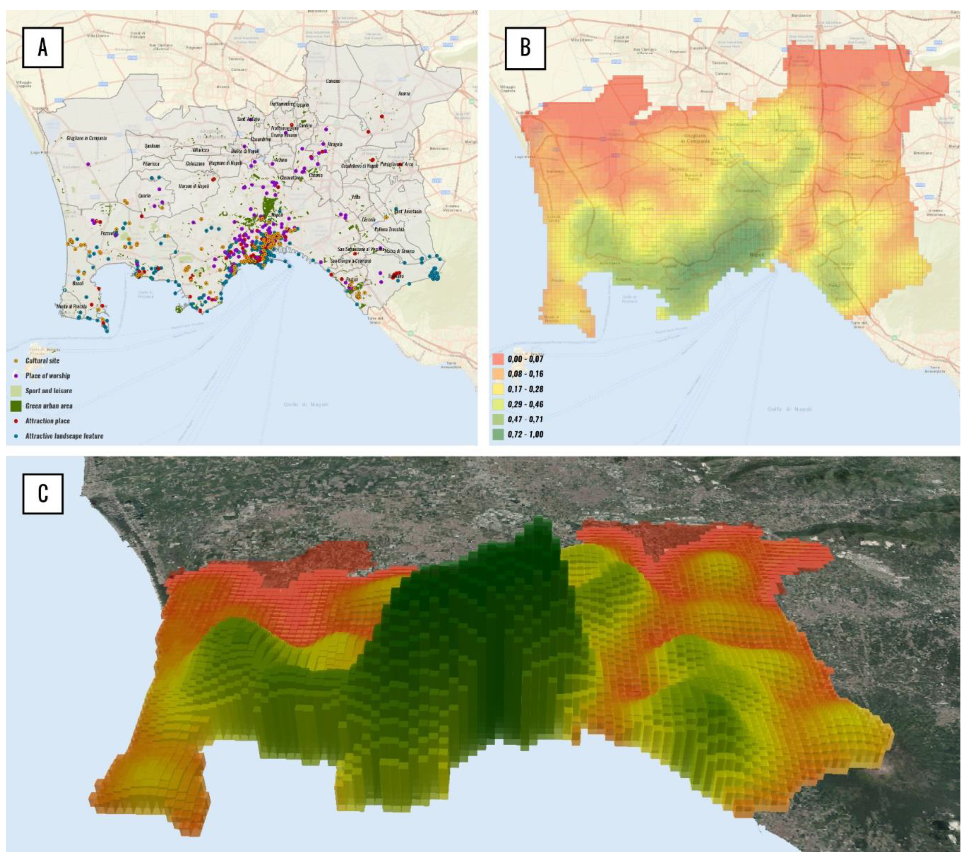
Figure 4 and Figure 5 highlight an excerpt of the 3D modelling for the focus area, zooming in on Naples city and overlapping the UES grid.
The operational steps allowed us to enhance the spatial visualisation of the urban morphology and, simultaneously, overlay the UES indicator grid with 3D building neighbourhoods.

4. Outcome

The AHP multi-criteria aggregation rules, as implemented by MASCOT, allowed for the mapping of the distribution of UES per function. The results of the applied approach focused on:
  • Assessing the multi-functionality levels per MMU of 25 hectares (500 × 500 m cell size, depending on the average dimension of the Naples districts; the overall dimension of the focus area, which is a multiple of the square cell; and the PC computational power);
  • Visualising the spatial distribution of services by applying the Euclidean distance method;
  • Planning scenarios for the spatial implementation of UES by considering the degree of suitability per MMU.
Table 2 shows the minimum (Min), maximum (Max), and standard deviation (St. Dev.) values of UES function for each municipality within the focus area.
A comparison of the data highlights that the Municipality of Naples had the maximum value of services for all three categories. In the case of Regulation functions, while it had the highest value, the standard deviation was also high, which implies deviation from the very significant average value (i.e., the areas with high regulative ecosystem values are interspersed with more urbanised areas with low levels of green features). Moreover, it is interesting to observe that the Municipality of Bacoli, which borders Naples city, had a very high value for the Regulation functions, with a slightly lower standard deviation, in comparison with Naples. This implies a more even distribution of such services within its boundaries. All the other municipalities had much lower values. The following figures show the 3D UES mapping results. The Regulation functions were evenly spatially distributed over the overall investigation area, but higher values can be detected in the south-western zones of the city, as shown in Figure 6. Figure 7 highlights the peaks of Carrier functions as being in the downtown of Naples. In these zones, transportation and tourism facilities are the densest, while the suburban areas are lacking in these types of facilities.
Figure 8 highlights the comparison among the UES values per function by overlapping the z-values of the grid. The three coloured gradients represent Regulation (green), Carrier (blue), and Information (red) services.
The north-eastern areas showed low values (or a lack of them) for Carrier and Information functions, while moderate values for Regulation functions balanced this gap. The null values in the north-western regions of the focus area can be attributed to the absence of services and the information gap.

5. Discussion

The proposed methodological approach underlines how UES classification and representation within a 3D GIS-based environment can support the processes of evaluation, planning, and monitoring by improving the visualisation of the spatial relationships of service allocation.
The 3D GIS-based modelling in the case study was intended to explain how certain information can be communicated more effectively, improving the level and quality of knowledge of decision-makers regarding the localisation, features, and status of UES.
The identification of UES and the classification of relevant spatial functions allowed us to define a framework for structuring site-specific knowledge through the selection of services representing local peculiarities.
The integration of GIS and MCDA supported the implementation of spatial assessments to investigate the UES and their relationships within the characteristics of the city system, referred to as MMU [43], which was used to identify a homogenous surface for analysis [42].
The elaboration of a Spatial Decision-Making Support System (SDMSS), in which GIS tools and the spatial multi-criteria AHP method interact and work together, produced a normalised index of UES per MMU. The processing of the cell-by-cell weighted sum and Euclidean distance among the spatial elements provided a relevant result to integrate different UES characteristics. At the same time, the number of the objects within the distance threshold and their weighted sum provided the weight per category per cell and was used to express the importance of the cell with respect to the Regulation, Carrier, and Information functions.
According to O’Sullivan and Unwin [100], the selection of different statistical units leads to totally different results, generating new patterns and spatial relationships between the features that shape the investigation area. An advantage of using a regular cell grid is combining the original mapping units with more accurate cells, in order to investigate the effects of urban changes at different scales. Indeed, the EEA has recognised that regular grids are very useful for understanding the spatial variability of phenomena, their mapping, and their evaluation [101].
Within the SDMSS, the implementation of MASCOT (based on the AHP multi-criteria aggregation rules) identified the potential to map the distribution of UES for each Regulation, Carrier, and Information function, as well as that to assess the multi-functionality levels. Indeed, MASCOT provided the opportunity to operationalise the pairwise comparison between different tiers and to spatially express the evaluation results.
The 3D visualisation of the spatial distribution of UES represents an innovative component of the methodological process, making the values of the three selected UES functions categories more easily understandable and communicable. The 3D visualisation can be considered a suitable way to analyse UES characteristics and to support the elaboration of planning and design alternatives, starting with the identification of enabling conditions. Our experimental study, applied to the city of Naples, made it possible to verify the significance of the role that 3D modelling can play in a virtual decisional environment, in terms of the communication of UES, as well as the democratisation and the negotiation of transformational choices [53]. The 3D modelling and virtual decisional environment involve the representation of UES, considering an inclusive approach in which all the involved stakeholders have the chance to understand the spatial changes in UES and to elicit values related to each understanding jointly. Conflicts in perception and preferred knowledge bases [102] emerge through a clear and effective representation supported by other deliberative methodologies to engage stakeholders and citizens in decision-making processes, while improving the expression of different preferences in a complex decision context [57,103,104]. Within a virtual decisional environment, the scale selected for the 3D modelling representation is crucial, as it determines the suitable detection of UES. Moreover, the size of the MMU makes the understanding of similar characteristics effective and their differences understandable, including the different boundaries of stakeholder concern.
At the same time, the main limitations of the proposed approach relate to:
The static visualisation of the maps, which requires complex processing and cannot be changed quickly for an interactive decision-making process;
The lack of different scenarios to be compared, as it is not feasible when equal weights have been assigned to spatial criteria (tiers);
Time-consuming processes related to the manipulation of stakeholder preferences and the sensitivity analysis (i.e., introducing or removing tiers, as influenced by stakeholder interests);
Loss of relevant information, data noise, and likely overfitting if the criteria/tiers are multiple or dispersed on several geographical entities.
Indeed, the proposed methodological approach allowed us to identify a SDMSS, combining the potentials of 3D modelling into a decisional GIS-environment with MCDA, highlighting the synergistic contribution that can be provided to improve the analysis and representation of UES and to support their evaluation for planning and monitoring. The interaction among different tools allowed for structuring a performing framework for UES, highlighting the opportunity to assess the status of services within the administrative boundaries of Naples city and its surroundings, and to guide the selection of new transformations and urban policies.

6. Conclusions

This study was conceived as the first step toward the further implementation of the 3D modelling approach. A better correlation between the UES and z-value must be tested, in order to explore the complexity of the urban spatial configuration and to improve the results of consequent decision-making processes.
The SDMSS incorporates 3D modelling as a central component. The third dimension included in the UES assessment identifies a relevant opportunity to understand the details of urban structure–function relationships, improving modelling and the visualisation of data and related impacts. The proposed methodological framework supports the evaluation, planning, and monitoring of UES within a 3D virtual environment, overcoming the limits of 2D representation and helping decision-makers to localise, assess, and manage urban development strategies.
The SDMSS addresses one of the main challenges in sustainability research related to the elaboration of spatial models, adapting to changes in managing sustainable transformations. The 3D virtual environment supports the representation of multiple services at the same location within a unique map, even if it does not enable the description of changes in services over time at present. The 3D modelling, conceived as an integral part of web-GIS, could allow for the inclusion of the time dimension and the visualisation of changes and transformations dynamically. At the same time, 3D modelling in a virtual environment allowed us to represent relationships between z-elevation values and specific UES spatially, highlighting the system of relationships between the heights of the buildings and the quality of services that each cell features.
One of the significant contributions offered by the SDMSS is the possibility of visualising UES trade-offs simultaneously, in order to identify opportunities linked to a sustainable spatial policy where economic, ecological, and social components should reach a balance.
Another result of applying the proposed model is the possibility to implement a multi-scale decision-making process, where the scale of analysis and assessment influences the problem definition and the related results, including different interests with respect to the issues addressed for each scale. The synthesis maps for each function—related to Regulation, Carrier, and Information services implemented with the aggregation rule of the spatial AHP—can be used to produce a normalised index of UES per cell. This index is the expression of a multi-scale assessment, incorporating different dimensions that are not present in single-scale assessments, including the selection and quantification of UES.
The spatial AHP method for aggregating (or even downscaling) to support comparison across scales establishes a mechanism for ensuring information flow across the scales of the assessment and integrating them. The multi-scale approach also tries to address the challenge related to stakeholder involvement and participation, adopting a more flexible process, as necessary to include different scales (i.e., political, economic, social, cultural, and environmental).
The AHP multi-criteria aggregation process was used for mapping the distribution of UES for each function, combining visual and non-visual information of the MMU. The results of the applied approach can support the elaboration of planning scenarios, considering the degree of suitability per MMU related to the selected UES.
Future developments of this research aim to stress some of the opportunities identified, such as including other cultural and social services, which are crucial for analysing and understanding urban dynamics. In this framework, one of the main challenges in sustainability research is to conceive models that are capable of adapting to changes in scale and recalibrating the selected indicators, depending on the degree of detail and data availability. Moreover, the multi-scale approach can be tested by including deliberative evaluative techniques that allow for considering conflicting stakeholder interests within the decision-making process.
Furthermore, integrated models may become the basis for computer games that engage players in decision-making, matching understanding to the evaluation [25] and supporting active interaction among different players (stakeholders). Indeed, integrated models can embed the trade-offs between ecological functions and the needs of citizens, eliciting stakeholder choices, favouring social interaction and dynamic modelling, and providing the opportunity for them to reflect on how they value the different trade-offs. A dynamic perspective for decision-support systems—oriented to improving dialogue and communication among stakeholders—could activate a mutual learning process within the play system and multiply interactions among different roles and point of views, from a plural and inclusive perspective.

Author Contributions

The authors jointly conceived and developed the approach and decided on the overall objective and structure of the paper: conceptualisation, M.C., R.M., and G.P.; methodology, M.C., R.M., and G.P.; software, R.M. and G.P.; validation, R.M. and G.P.; formal analysis, R.M.; investigation, G.P.; resources, G.P.; data curation, R.M.; writing—original draft preparation, G.P. and R.M.; writing—review and editing, M.C. and G.P.; visualisation, R.M. and G.P.; supervision, M.C. All authors have read and agreed to the published version of the manuscript.

Funding

This research received no external funding.

Acknowledgments

The authors would like to express thanks for the interesting suggestions and important comments received from the five anonymous referees, which have allowed us to improve and integrate the paper and to achieve a more significant final result.

Conflicts of Interest

The authors declare no conflict of interest.

References

  1. EU. Biodiversity Strategy for 2030. Bringing Nature Back into Our Lives. Available online: https://eur-lex.europa.eu/legal-content/EN/TXT/?qid=1590574123338&uri=CELEX:52020DC0380 (accessed on 18 July 2020).
  2. OECD. Biodiversity: Finance and the Economic and Business Case for Action. Report Prepared for the G7 Environment Ministers’ Meeting. 5–6 May 2019. Available online: https://www.oecd.org/env/resources/biodiversity/biodiversity-finance-and-the-economic-and-business-case-for-action.htm (accessed on 18 July 2020).
  3. Potschin, M.; Haines-Young, R. Defining and measuring ecosystem services. In Routledge Handbook of Ecosystem Services; Potschin, M., Haines-Young, R., Fish, R., Turner, R.K., Eds.; Routledge: London, UK; New York, NY, USA, 2016; pp. 25–44. [Google Scholar]
  4. Ghazoul, J. Recognising the complexities of ecosystem management and the ecosystem service concept. Gaia-Ecol. Perspect. Sci. Soc. 2007, 16, 215–221. [Google Scholar] [CrossRef]
  5. Costanza, R. Ecosystem services: Multiple classification systems are needed. Biol. Conserv. 2008, 141, 350–352. [Google Scholar] [CrossRef]
  6. Norgaard, R.B. Ecosystem services: From eye-opening metaphor to complexity blinder. Ecol. Econ. 2010, 69, 1219–1227. [Google Scholar] [CrossRef]
  7. Lang, D.J.; Wiek, A.; Bergmann, M.; Stauffacher, M.; Martens, P.; Moll, P.; Swilling, M.; Thomas, G.J. Transdisciplinary research in sustainability science: Practice, principles, and challenges. Sustain. Sci. 2012, 7, 25–43. [Google Scholar] [CrossRef]
  8. Abson, D.J.; von Wehrden, H.; Baumgärtner, S.; Fischer, J.; Hanspach, J.; Härdtle, W.; Heinrichs, H.; Klein, A.M.; Lang, D.J.; Martens, P.; et al. Ecosystem services as a boundary object for sustainability. Ecol. Econ. 2014, 103, 29–37. [Google Scholar] [CrossRef]
  9. Costanza, R. Social Goals and the Valuation of Ecosystem Services. Ecosystems 2000, 3, 4–10. [Google Scholar] [CrossRef]
  10. Costanza, R. Valuing natural capital and ecosystem services toward the goals of efficiency, fairness, and sustainability. Ecosyst. Serv. 2020, 43, 101096. [Google Scholar] [CrossRef]
  11. MEA. Ecosystems and Human Well-being: Synthesis; Island Press: Washington, DC, USA, 2005. [Google Scholar]
  12. Zermoglio, M.F.; Biggs, R.; Vicente, L. The Multiscale Approach. Ecosyst. Hum. Well Being 2005, 61. [Google Scholar]
  13. Gómez-Baggethun, E.; Barton, D.N. Classifying and valuing ecosystem services for urban planning. Ecol. Econ. 2013, 86, 235–245. [Google Scholar] [CrossRef]
  14. Larondelle, N.; Haase, D. Urban ecosystem services assessment along a rural–urban gradient: A cross-analysis of European cities. Ecol. Indic. 2013, 29, 179–190. [Google Scholar] [CrossRef]
  15. Kremer, P.; Hamstead, Z.; Haase, D.; McPhearson, T.; Frantzeskaki, N.; Andersson, E.; Kabisch, N.; Larondelle, N.; Rall, E.L.; Voigt, A. Key insights for the future of urban ecosystem services research. Ecol. Soc. 2016, 21, 21. [Google Scholar] [CrossRef] [Green Version]
  16. Kourdounouli, C.; Jönsson, A.M. Urban ecosystem conditions and ecosystem services–a comparison between large urban zones and city cores in the EU. J. Environ. Plan. Manag. 2020, 63, 798–817. [Google Scholar] [CrossRef]
  17. Tan, P.Y.; Zhang, J.; Masoudi, M.; Alemu, J.B.; Edwards, P.J.; Grêt-Regamey, A.; Richards, D.R.; Saunders, J.; Song, X.P.; Wong, L.W. A conceptual framework to untangle the concept of urban ecosystem services. Landsc. Urban. Plan. 2020, 200, 103837. [Google Scholar] [CrossRef] [PubMed]
  18. Luederitz, C.; Brink, E.; Gralla, F.; Hermelingmeier, V.; Meyer, M.; Niven, L.; Panzer, L.; Partelow, S.; Rau, A.; Sasaki, R.; et al. A review of urban ecosystem services: Six key challenges for future research. Ecosyst. Serv. 2015, 14, 98–112. [Google Scholar] [CrossRef] [Green Version]
  19. Antognelli, S.; Vizzari, M. Ecosystem and urban services for landscape liveability: A model for quantification of stakeholders’ perceived importance. Land Use Policy 2016, 50, 277–292. [Google Scholar] [CrossRef]
  20. Vejre, H.; Jensen, F.S.; Thorsen, B.J. Demonstrating the importance of intangible ecosystem services from peri-urban landscapes. Ecol. Complex. 2010, 7, 338–348. [Google Scholar] [CrossRef]
  21. Ostrom, E. A General Framework for Analyzing Sustainability of Social-Ecological Systems. Science 2009, 325, 419–422. [Google Scholar] [CrossRef]
  22. Ahern, J.; Cilliers, S.; Niemelä, J. The concept of ecosystem services in adaptive urban planning and design: A framework for supporting innovation. Landsc. Urban. Plan. 2014, 125, 254–259. [Google Scholar] [CrossRef] [Green Version]
  23. Boumans, R.; Roman, J.; Altman, I.; Kaufman, L. The Multiscale Integrated Model of Ecosystem Services (MIMES): Simulating the interactions of coupled human and natural systems. Ecosyst. Serv. 2015, 12, 30–41. [Google Scholar] [CrossRef]
  24. Haase, D.; Larondelle, N.; Andersson, E.; Artmann, M.; Borgström, S.; Breuste, J.; Gomez-Baggethun, E.; Gren, Å.; Hamstead, Z.; Hansen, R.; et al. A Quantitative Review of Urban Ecosystem Service Assessments: Concepts, Models, and Implementation. AMBIO 2014, 43, 413–433. [Google Scholar] [CrossRef] [Green Version]
  25. Costanza, R.; de Groot, R.; Braat, L.; Kubiszewski, I.; Fioramonti, L.; Sutton, P.; Farber, S.; Grasso, M. Twenty years of ecosystem services: How far have we come and how far do we still need to go? Ecosyst. Serv. 2017, 28, 1–16. [Google Scholar] [CrossRef]
  26. De Groot, R.S.; Alkemade, R.; Braat, L.; Hein, L.; Willemen, L. Challenges in integrating the concept of ecosystem services and values in landscape planning, management and decision making. Ecol. Complex. 2010, 7, 260–272. [Google Scholar] [CrossRef]
  27. Klein, T.M.; Celio, E.; Grêt-Regamey, A. Ecosystem services visualization and communication: A demand analysis approach for designing information and conceptualizing decision support systems. Ecosyst. Serv. 2015, 13, 173–183. [Google Scholar] [CrossRef]
  28. Elliot, T.B.; Almenar, J.B.; Niza, S.; Proença, V.; Rugani, B. Pathways to Modelling Ecosystem Services within an Urban Metabolism Framework. Sustainability 2019, 11, 2766. [Google Scholar] [CrossRef] [Green Version]
  29. Adda, P.; Mioc, D.; Anton, F.; McGillivray, E.; Morton, A.; Fraser, D.; Eb, C. 3D flood-risk models of government infrastructure. In Proceedings of the WebMGS 2010: 1st International Workshop on Pervasive Web Mapping, Geoprocessing and Services, Como, Italy, 26–27 August 2010; Volume XXXVIII-4, pp. 6–11. [Google Scholar]
  30. Middel, A.; Häb, K.; Brazel, A.J.; Martin, C.A.; Guhathakurta, S. Impact of urban form and design on mid-afternoon microclimate in Phoenix Local Climate Zones. Landsc. Urban. Plan. 2014, 122, 16–28. [Google Scholar] [CrossRef]
  31. Balzan, M.V.; Caruana, J.; Zammit, A. Assessing the capacity and flow of ecosystem services in multifunctional landscapes: Evidence of a rural-urban gradient in a Mediterranean small island state. Land Use Policy 2018, 75, 711–725. [Google Scholar] [CrossRef]
  32. Cerreta, M.; Panaro, S. From Perceived Values to Shared Values: A Multi-Stakeholder Spatial Decision Analysis (M-SSDA) for Resilient Landscapes. Sustainability 2017, 9, 1113. [Google Scholar] [CrossRef] [Green Version]
  33. Geneletti, D. Reasons and options for integrating ecosystem services in strategic environmental assessment of spatial planning. Int. J. Biodivers. Sci. Ecosyst. Serv. Manag. 2011, 7, 143–149. [Google Scholar] [CrossRef] [Green Version]
  34. Cerreta, M.; Poli, G. Landscape Services Assessment: A Hybrid Multi-Criteria Spatial Decision Support System (MC-SDSS). Sustainability 2017, 9, 1311. [Google Scholar] [CrossRef] [Green Version]
  35. Scorza, F.; Pilogallo, A.; Saganeiti, L.; Murgante, B.; Pontrandolfi, P. Comparing the territorial performances of renewable energy sources’ plants with an integrated ecosystem services loss assessment: A case study from the Basilicata region (Italy). Sustain. Cities Soc. 2020, 56, 102082. [Google Scholar] [CrossRef]
  36. Grêt-Regamey, A.; Celio, E.; Klein, T.M.; Wissen Hayek, U. Understanding ecosystem services trade-offs with interactive procedural modeling for sustainable urban planning. Landsc. Urban. Plan. 2013, 109, 107–116. [Google Scholar] [CrossRef]
  37. Vuuren, D.P.v.; Sala, O.E.; Pereira, H.M. The Future of Vascular Plant Diversity Under Four Global Scenarios. Ecol. Soc. 2006, 11, 25. [Google Scholar] [CrossRef] [Green Version]
  38. Chun, B.; Guldmann, J.M. Spatial statistical analysis and simulation of the urban heat island in high-density central cities. Landsc. Urban. Plan. 2014, 125, 76–88. [Google Scholar] [CrossRef]
  39. Hayek, U.W. Which is the Appropriate 3D Visualization Type for Participatory Landscape Planning Workshops? A Portfolio of Their Effectiveness. Environ. Plan. B Plan. Des. 2011, 38, 921–939. [Google Scholar] [CrossRef]
  40. Scholes, R.J.; Reyers, B.; Biggs, R.; Spierenburg, M.J.; Duriappah, A. Multi-scale and cross-scale assessments of social–ecological systems and their ecosystem services. Curr. Opin. Environ. Sustain. 2013, 5, 16–25. [Google Scholar] [CrossRef]
  41. Malczewski, J.; Rinner, C. Multicriteria Decision Analysis in Geographic Information Science; Springer: Berlin/Heidelberg, Germany, 2015. [Google Scholar]
  42. Barreto, L.; Ribeiro, M.C.; Veldkamp, A.; van Eupen, M.; Kok, K.; Pontes, E. Exploring effective conservation networks based on multi-scale planning unit analysis. A case study of the Balsas sub-basin, Maranhão State, Brazil. Ecol. Indic. 2010, 10, 1055–1063. [Google Scholar] [CrossRef]
  43. Knight, J.F.; Lunetta, R.S. An experimental assessment of minimum mapping unit size. IEEE Trans. Geosci. Remote Sens. 2003, 41, 2132–2134. [Google Scholar] [CrossRef]
  44. Jacobs, S.; Martín-López, B.; Barton, D.N.; Dunford, R.; Harrison, P.A.; Kelemen, E.; Saarikoski, H.; Termansen, M.; García-Llorente, M.; Gómez-Baggethun, E.; et al. The means determine the end–Pursuing integrated valuation in practice. Ecosyst. Serv. 2018, 29, 515–528. [Google Scholar] [CrossRef]
  45. Braat, L.; Gómez-Baggethun, E.; Martín-López, B.; Barton, D.; García-Llorente, M.; Kelemen, E.; Saarikoski, H. Framework for Integration of Valuation Methods to Assess Ecosystem Service Policies. European Commission EU FP7 OpenNESS Project Deliverable. 2014. 4.2. Available online: http://www.openness-project.eu/sites/default/files/OpenNESS%20D4.2%20Framework_%20Integrated_Valuation_Final_Draft_March_23-2015.pdf (accessed on 18 June 2020).
  46. Brown, G.; Fagerholm, N. Empirical PPGIS/PGIS mapping of ecosystem services: A review and evaluation. Ecosyst. Serv. 2015, 13, 119–133. [Google Scholar] [CrossRef]
  47. Kenter, J.O. Shared, plural and cultural values. Ecosyst. Serv. 2016, 21, 175–183. [Google Scholar] [CrossRef]
  48. Kenter, J.O.; Bryce, R.; Christie, M.; Cooper, N.; Hockley, N.; Irvine, K.N.; Fazey, I.; O’Brien, L.; Orchard-Webb, J.; Ravenscroft., N.; et al. Shared values and deliberative valuation: Future directions. Ecosyst. Serv. 2016, 21, 358–371. [Google Scholar] [CrossRef] [Green Version]
  49. Jacobs, S.; Dendoncker, N.; Keune, H. Ecosystem Services: Global Issues, Local Practices; Elsevier: Amsterdam, The Netherlands, 2013. [Google Scholar]
  50. Alavipanah, S.; Haase, D.; Lakes, T.; Qureshi, S. Integrating the third dimension into the concept of urban ecosystem services: A review. Ecol. Indic. 2017, 72, 374–398. [Google Scholar] [CrossRef]
  51. Biljecki, F.; Stoter, J.; Ledoux, H.; Zlatanova, S.; Çöltekin, A. Applications of 3D city models: State of the art review. Isprs Int. J. Geo-Inf. 2015, 4, 2842–2889. [Google Scholar] [CrossRef] [Green Version]
  52. MEA. Ecosystems and Human Well-Being: A Framework for Assessment; Island Press: Washington, DC, USA, 2003. [Google Scholar]
  53. McHale, M.R.; Beck, S.M.; Pickett, S.T.A.; Childers, D.L.; Cadenasso, M.L.; Rivers, L.; Swemmer, L.; Ebersohn, L.; Twine, W.; Bunn, D.N. Democratization of ecosystem services—A radical approach for assessing nature’s benefits in the face of urbanization. Ecosyst. Health Sustain. 2018, 4, 115–131. [Google Scholar] [CrossRef] [Green Version]
  54. Nahlik, A.M.; Kentula, M.E.; Fennessy, M.S.; Landers, D.H. Where is the consensus? A proposed foundation for moving ecosystem service concepts into practice. Ecol. Econ. 2012, 77, 27–35. [Google Scholar] [CrossRef]
  55. Reyers, B.; Nel, J.L.; O’Farrell, P.J.; Sitas, N.; Nel, D.C. Navigating complexity through knowledge coproduction: Mainstreaming ecosystem services into disaster risk reduction. Proc. Natl. Acad. Sci. USA 2015, 112, 7362–7368. [Google Scholar] [CrossRef] [PubMed] [Green Version]
  56. Cowling, R.M.; Egoh, B.; Knight, A.T.; O’Farrell, P.J.; Reyers, B.; Rouget, M.; Roux, D.J.; Welz, A.; Wilhelm-Rechman, A. An operational model for mainstreaming ecosystem services for implementation. Proc. Natl. Acad. Sci. USA 2008, 105, 9483–9488. [Google Scholar] [CrossRef] [Green Version]
  57. Turner, N.J.; Gregory, R.; Brooks, C.; Failing, L.; Satterfield, T. From invisibility to transparency: Identifying the implications. Ecol. Soc. 2008, 13, 13. [Google Scholar] [CrossRef]
  58. Carpenter, S.R.; Mooney, H.A.; Agard, J.; Capistrano, D.; DeFries, R.S.; Díaz, S.; Dietz, T.; Duraiappah, A.K.; Oteng-Yeboah, A.; Pereira, H.M. Science for managing ecosystem services: Beyond the Millennium Ecosystem Assessment. Proc. Natl. Acad. Sci. USA 2009, 106, 1305–1312. [Google Scholar] [CrossRef] [Green Version]
  59. Maynard, S.; James, D.; Davidson, A. The Development of an Ecosystem Services Framework for South East Queensland. Environ. Manag. 2010, 45, 881–895. [Google Scholar] [CrossRef]
  60. Pascua, P.a.; McMillen, H.; Ticktin, T.; Vaughan, M.; Winter, K.B. Beyond services: A process and framework to incorporate cultural, genealogical, place-based, and indigenous relationships in ecosystem service assessments. Ecosyst. Serv. 2017, 26, 465–475. [Google Scholar] [CrossRef]
  61. Goodchild, M.F.; Li, L. Assuring the quality of volunteered geographic information. Spat. Stat. 2012, 1, 110–120. [Google Scholar] [CrossRef]
  62. Birch, C.P.D.; Oom, S.P.; Beecham, J.A. Rectangular and hexagonal grids used for observation, experiment and simulation in ecology. Ecol. Model. 2007, 206, 347–359. [Google Scholar] [CrossRef]
  63. Englund, O.; Berndes, G.; Cederberg, C. How to analyse ecosystem services in landscapes—A systematic review. Ecol. Indic. 2017, 73, 492–504. [Google Scholar] [CrossRef]
  64. Li, X.; Zhou, W.; Ouyang, Z. Relationship between land surface temperature and spatial pattern of greenspace: What are the effects of spatial resolution? Landsc. Urban. Plan. 2013, 114, 1–8. [Google Scholar] [CrossRef]
  65. Zhou, G.; Song, C.; Simmers, J.; Cheng, P. Urban 3D GIS From LiDAR and digital aerial images. Comput. Geosci. 2004, 30, 345–353. [Google Scholar] [CrossRef]
  66. Popovic, D.; Govedarica, M.; Jovanovic, D.; Radulovic, A.; Simeunovic, V. 3D Visualization of Urban Area Using Lidar Technology and CityGML. IOP Conf. Ser. Earth Environ. Sci. 2017, 95, 042006. [Google Scholar] [CrossRef]
  67. Arsanjani, J.J.; Mooney, P.; Zipf, A.; Schauss, A. Quality assessment of the contributed land use information from OpenStreetMap versus authoritative datasets. In OpenStreetMap in GIScience; Springer: Berlin/Heidelberg, Germany, 2015; pp. 37–58. [Google Scholar]
  68. Fan, H.; Zipf, A.; Fu, Q.; Neis, P. Quality assessment for building footprints data on OpenStreetMap. Int. J. Geogr. Inf. Sci. 2014, 28, 700–719. [Google Scholar] [CrossRef]
  69. Fan, H.; Zipf, A. Modelling the world in 3D from VGI/Crowdsourced data. In European Handbook of Crowdsourced Geographic Information; Ubiquity Press: London, UK, 2016; pp. 435–446. [Google Scholar]
  70. Campagna, M. Social Media Geographic Information: Why social is special when it goes spatial. In European Handbook of Crowdsourced Geographic Information; Capineri, C., Haklay, M., Huang, H., Antoniou, V., Kettunen, J., Ostermann, F., Purves, R., Eds.; Ubiquity Press: London, UK, 2016; pp. 45–54. [Google Scholar]
  71. Hecht, R.; Kunze, C.; Hahmann, S. Measuring completeness of building footprints in OpenStreetMap over space and time. Isprs Int. J. Geo-Inf. 2013, 2, 1066–1091. [Google Scholar] [CrossRef]
  72. Fonte, C.C.; Antoniou, V.; Bastin, L.; Estima, J.; Arsanjani, J.J.; Bayas, J.-C.L.; See, L.; Vatseva, R. Assessing VGI data quality. Mapp. Citiz. Sens. 2017, 137–163. [Google Scholar]
  73. Wang, R. 3D building modeling using images and LiDAR: A review. Int. J. Image Data Fusion 2013, 4, 273–292. [Google Scholar] [CrossRef]
  74. Shiode, N. 3D urban models: Recent developments in the digital modelling of urban environments in three-dimensions. GeoJournal 2000, 52, 263–269. [Google Scholar] [CrossRef]
  75. Shingare, P.P.; Kale, S. Review on digital elevation model. Int. J. Mod. Eng. Res. IJMER 2013, 3, 2412–2418. [Google Scholar]
  76. Mallet, C.; David, N. 7-Digital Terrain Models Derived from Airborne LiDAR Data. In Optical Remote Sensing of Land Surface; Baghdadi, N., Zribi, M., Eds.; Elsevier: Amsterdam, The Netherlands, 2016; pp. 299–319. [Google Scholar]
  77. Saaty, T.L. The seven pillars of the analytic hierarchy process. In Multiple Criteria Decision Making in the New Millennium; Springer: Berlin/Heidelberg, Germany, 2001; pp. 15–37. [Google Scholar]
  78. Mele, R.; Poli, G. The Effectiveness of Geographical Data in Multi-Criteria Evaluation of Landscape Services@. Data 2017, 2, 9. [Google Scholar] [CrossRef] [Green Version]
  79. Urban Atlas 2018—Copernicus Land Monitoring Service. Available online: https://land.copernicus.eu/ (accessed on 1 December 2018).
  80. MEA. Current State and Trends; Island Press: Washington, DC, USA, 2005. [Google Scholar]
  81. TEEB. Mainstreaming the Economics of Nature: A Synthesis of the Approach, Conclusions and Recommendations of TEEB; Progress Press: Geneva, Switzerland, 2010; Available online: http://www.teebweb.org/publication/mainstreaming-the-economics-of-nature-a-synthesis-of-the-approach-conclusions-and-recommendations-of-teeb/ (accessed on 18 June 2020).
  82. Hermann, A.; Schleifer, S.; Wrbka, T. The Concept of Ecosystem Services Regarding Landscape Research: A Review. Living Rev. Landsc. Res. 2011, 5, 1–37. [Google Scholar] [CrossRef] [Green Version]
  83. Lamarque, P.; Quétier, F.; Lavorel, S. The diversity of the ecosystem services concept and its implications for their assessment and management. C. R. Biol. 2011, 334, 441–449. [Google Scholar] [CrossRef]
  84. Costanza, R.; d’Arge, R.; de Groot, R.; Farber, S.; Grasso, M.; Hannon, B.; Limburg, K.; Naeem, S.; O’Neill, R.V.; Paruelo, J.; et al. The value of the world’s ecosystem services and natural capital. Nature 1997, 387, 253–260. [Google Scholar] [CrossRef]
  85. Wallace, K.J. Classification of ecosystem services: Problems and solutions. Biol. Conserv. 2007, 139, 235–246. [Google Scholar] [CrossRef] [Green Version]
  86. de Groot, R.S.; Wilson, M.A.; Boumans, R.M.J. A typology for the classification, description and valuation of ecosystem functions, goods and services. Ecol. Econ. 2002, 41, 393–408. [Google Scholar] [CrossRef] [Green Version]
  87. De Groot, R. Function-analysis and valuation as a tool to assess land use conflicts in planning for sustainable, multi-functional landscapes. Landsc. Urban. Plan. 2006, 75, 175–186. [Google Scholar] [CrossRef]
  88. Haines-Young, R.; Potschin, M. The links between biodiversity, ecosystem services and human well-being. Ecosyst. Ecol. A New Synth. 2010, 1, 110–139. [Google Scholar]
  89. Potschin, M.; Haines-Young, R. Landscapes, sustainability and the place-based analysis of ecosystem services. Landsc. Ecol. 2013, 28, 1053–1065. [Google Scholar] [CrossRef]
  90. Haines-Young, R.; Potschin, M. Common international classification of ecosystem services (CICES, Version 4.1). Eur. Environ. Agency 2012, 33, 107. [Google Scholar]
  91. Daily, G.C.; Polasky, S.; Goldstein, J.; Kareiva, P.M.; Mooney, H.A.; Pejchar, L.; Ricketts, T.H.; Salzman, J.; Shallenberger, R. Ecosystem services in decision making: Time to deliver. Front. Ecol. Environ. 2009, 7, 21–28. [Google Scholar] [CrossRef] [Green Version]
  92. Rall, E.L.; Kabisch, N.; Hansen, R. A comparative exploration of uptake and potential application of ecosystem services in urban planning. Ecosyst. Serv. 2015, 16, 230–242. [Google Scholar] [CrossRef]
  93. Costanza, R. Ecosystem health and ecological engineering. Ecol. Eng. 2012, 45, 24–29. [Google Scholar] [CrossRef] [Green Version]
  94. Jones, L.; Norton, L.; Austin, Z.; Browne, A.; Donovan, D.; Emmett, B.; Grabowski, Z.; Howard, D.; Jones, J.; Kenter, J. Stocks and flows of natural and human-derived capital in ecosystem services. Land Use Policy 2016, 52, 151–162. [Google Scholar] [CrossRef]
  95. Pickett, S.; Boone, C.G.; McGrath, B.P.; Cadenasso, M.; Childers, D.L.; Ogden, L.A.; McHale, M.; Grove, J.M. Ecological science and transformation to the sustainable city. Cities 2013, 32, S10–S20. [Google Scholar] [CrossRef]
  96. Tan, P.Y.; Bin Abdul Hamid, A.R. Urban ecological research in Singapore and its relevance to the advancement of urban ecology and sustainability. Landsc. Urban. Plan. 2014, 125, 271–289. [Google Scholar] [CrossRef]
  97. Vallés-Planells, M.; Galiana, F.; Van Eetvelde, V. A Classification of Landscape Services to Support Local Landscape Planning. Ecol. Soc. 2014, 19, 19. [Google Scholar] [CrossRef] [Green Version]
  98. Verhagen, W. Managing our Land for Multiple Ecosystem Services: Identifying Priority Areas and Actions to Maintain Ecosystem Services Across Europe; Vrije Universiteit Amsterdam: Amsterdam, The Netherlands, 2019. [Google Scholar]
  99. Lacroix, P.; Santiago, H.; Ray, N. Mascot: Multi-criteria analytical scoring tool for arcgis desktop. Int. J. Inf. Technol. Decis. Mak. 2014, 13, 1135–1159. [Google Scholar] [CrossRef]
  100. O’Sullivan, D.; Unwin, D.J. Geographic Information Analysis and Spatial Data; Wiley Online Library: Hoboken, NJ, USA, 2010; pp. 1–32. [Google Scholar]
  101. EEA. Assistance to the EEA in the Production of the New CORINE Land Cover (CLC) Inventory, Including the Support to the Harmonisation of National Monitoring for Integration at Paneuropean Level–Geometric Test Case and Grid Approach; EEA: Copenhagen, Denmark, 2015. [Google Scholar]
  102. Haywood, B.K.; Besley, J.C. Education, outreach, and inclusive engagement: Towards integrated indicators of successful program outcomes in participatory science. Public Underst. Sci. 2014, 23, 92–106. [Google Scholar] [CrossRef] [PubMed]
  103. Bunse, L.; Rendon, O.; Luque, S. What can deliberative approaches bring to the monetary valuation of ecosystem services? A literature review. Ecosyst. Serv. 2015, 14, 88–97. [Google Scholar] [CrossRef]
  104. Pascual, U.; Balvanera, P.; Díaz, S.; Pataki, G.; Roth, E.; Stenseke, M.; Watson, R.T.; Başak Dessane, E.; Islar, M.; Kelemen, E.; et al. Valuing nature’s contributions to people: The IPBES approach. Curr. Opin. Environ. Sustain. 2017, 26–27, 7–16. [Google Scholar] [CrossRef] [Green Version]
Figure 1. The methodological workflow.
Applsci 10 06205 g001
Figure 2. Larger Urban Zones (LUZ) of Naples (Italy): a case study.
Applsci 10 06205 g002
Figure 3. (A) Information Services pre-processed map, (B) geodetic grid (500 × 500 m) with standardised indicator values in the range of 0–1, and (C) 3D visualisation of Information Services.
Applsci 10 06205 g003
Figure 4. Excerpt of the 3D city model with the Urban Ecosystem Services (UES) grid overlapped. The spatial relationships among building z-values and Regulation Services cell values are visualised.
Applsci 10 06205 g004
Figure 5. Excerpt of the 3D city model with the UES grid overlapped. The spatial relationships among building z-values and Regulation Services cell values are visualised.
Applsci 10 06205 g005
Figure 6. 3D visualisation of Regulation Services values with Jenks natural breaks categorisation. The colour gradient and histogram height show high (green) and low (red) UES values.
Applsci 10 06205 g006
Figure 7. 3D visualisation of Carrier Services values with Jenks natural breaks categorisation. The colour gradient and histogram height show high (green) and low (red) UES values.
Applsci 10 06205 g007
Figure 8. 3D visualisation of Regulation (green), Carrier (blue), and Information (red) service values with Jenks natural breaks categorisation. The overlay allows for visualising trade-offs among services at an overall level.
Applsci 10 06205 g008
Table 1. Urban Ecosystem Service indicators.
Urban Ecosystem Service FunctionsTierUnit of
Measure
Geometric EntityDistance Threshold
(DT)
Source
RegulationEnvironmental protection areaSq. kmPolygon2500Natura 2000—EC
WaterbodySq. kmPolygon300Urban Atlas—EEA
ForestSq. kmPolygon2500Urban Atlas—EEA
Land without current useSq. kmPolygon100Urban Atlas—EEA
WaterwayKmLine300OpenStreetMap
CarrierRailwayKmLine100OpenStreetMap
RoadKmLine100OpenStreetMap
AirportSq. kmPolygon1000Urban Atlas—EEA
PortSq. kmPolygon1000Urban Atlas—EEA
Bus/underground stopNumberPoint500OpenStreetMap
Mineral extraction siteSq. kmPolygon100OpenStreetMap
Habitation densityBuildings per sq. kmPolygon100Urban Atlas—EEA
Waste disposalSq. kmPolygon100OpenStreetMap
Tourism facilityNumberPoint500OpenStreetMap
InformationCultural siteNumberPoint2000OpenStreetMap
Place of worshipNumberPoint500OpenStreetMap
Sport and leisureSq. kmPolygon500Urban Atlas—EEA
Green urban areaSq. kmPolygon1000Urban Atlas—EEA
Attraction placeNumberPoint500OpenStreetMap
Attractive landscape featureNumberPoint1000Panoramio/Flickr
Table 2. Urban Ecosystem Services values standardised per municipality.
MunicipalityRegulation FunctionCarrier FunctionInformation Function
MinMaxSt. Dev.MinMaxSt. Dev.MinMaxSt. Dev.
Acerra0.0000.4600.1040.0000.2980.0510.0000.1420.036
Afragola0.0000.3720.1050.0000.2710.0780.0150.2980.084
Arzano0.0080.2590.0570.0040.2140.0620.1200.3430.064
Bacoli0.1270.9870.1840.0030.1780.0440.0420.2020.034
Caivano0.0000.2550.0610.0000.2720.0630.0000.1880.044
Calvizzano0.0000.4760.1300.0420.2060.0530.0440.1330.022
Cardito0.0640.3610.0840.0800.2320.0370.1520.2130.017
Casalnuovo di Napoli0.0000.3720.0950.0050.1150.0280.0250.1160.022
Casandrino0.0120.2960.0840.0040.2520.0760.1210.2500.030
Casavatore0.0170.2680.0740.1190.2590.0400.2530.3870.037
Casoria0.0000.4620.1080.0070.2600.0750.0250.3150.091
Cercola0.0040.3240.0920.0500.1640.0290.1350.2530.032
Crispano0.0000.2210.0660.0010.2610.0830.0550.2120.049
Ercolano0.0000.6480.1780.0000.2180.0550.0510.3510.061
Frattamaggiore0.0000.2980.0810.0110.2620.0710.1050.2130.027
Frattaminore0.0000.2210.0730.0090.2340.0720.0490.1910.040
Giugliano in Campania0.0000.6720.1160.0000.2110.0430.0000.2480.042
Grumo Nevano0.0000.1050.0360.0180.2000.0580.1210.1970.023
Marano di Napoli0.0000.6080.1910.0210.2040.0370.0100.1430.037
Massa di Somma0.0400.6330.1890.0000.2310.0720.0680.2080.036
Melito di Napoli0.0210.3060.0810.0190.2050.0440.1110.2820.040
Monte di Procida0.1270.4730.1100.0030.1540.0410.0470.1300.025
Mugnano di Napoli0.0140.4970.1200.0600.2640.0490.0870.2510.038
Napoli (Naples)0.0001.0000.2160.0021.0000.1430.0311.0000.245
Pollena Trocchia0.0000.5400.1270.0000.1840.0490.0610.1970.035
Pomigliano d’Arco0.0000.3300.0820.0000.2610.0580.0020.1160.027
Portici0.0180.3550.1150.0210.1920.0440.1890.3930.060
Pozzuoli0.0930.6930.1130.0010.2060.0350.0670.4230.094
Qualiano0.0000.1710.0390.0050.2600.0690.0040.1290.039
Quarto0.0000.4640.1550.0380.1500.0250.0080.2030.054
San Giorgio a C.0.0000.3290.0930.0480.1830.0320.1950.3570.036
S. Sebastiano al V.0.0000.6030.1700.0230.2470.0610.0890.2540.057
Sant’Anastasia0.0000.3720.0820.0000.2080.0430.0200.1610.036
Sant’Antimo0.0020.3210.0990.0160.2520.0700.0260.2070.051
Villaricca0.0000.1670.0520.0160.2060.0530.0040.1350.041
Volla0.0000.3740.0920.0050.1520.0410.0270.2570.063

