A Spring Search Algorithm Applied to Engineering Optimization Problems

 ,
,  , , ,
, , ,  ,
,  ,
,  and
and
Abstract
1. Introduction
2. A Brief History of Intelligent Algorithms
2.1. Swarm-Based Algorithms
2.2. Evolution-Based Algorithms
2.3. Physics-Based Algorithms
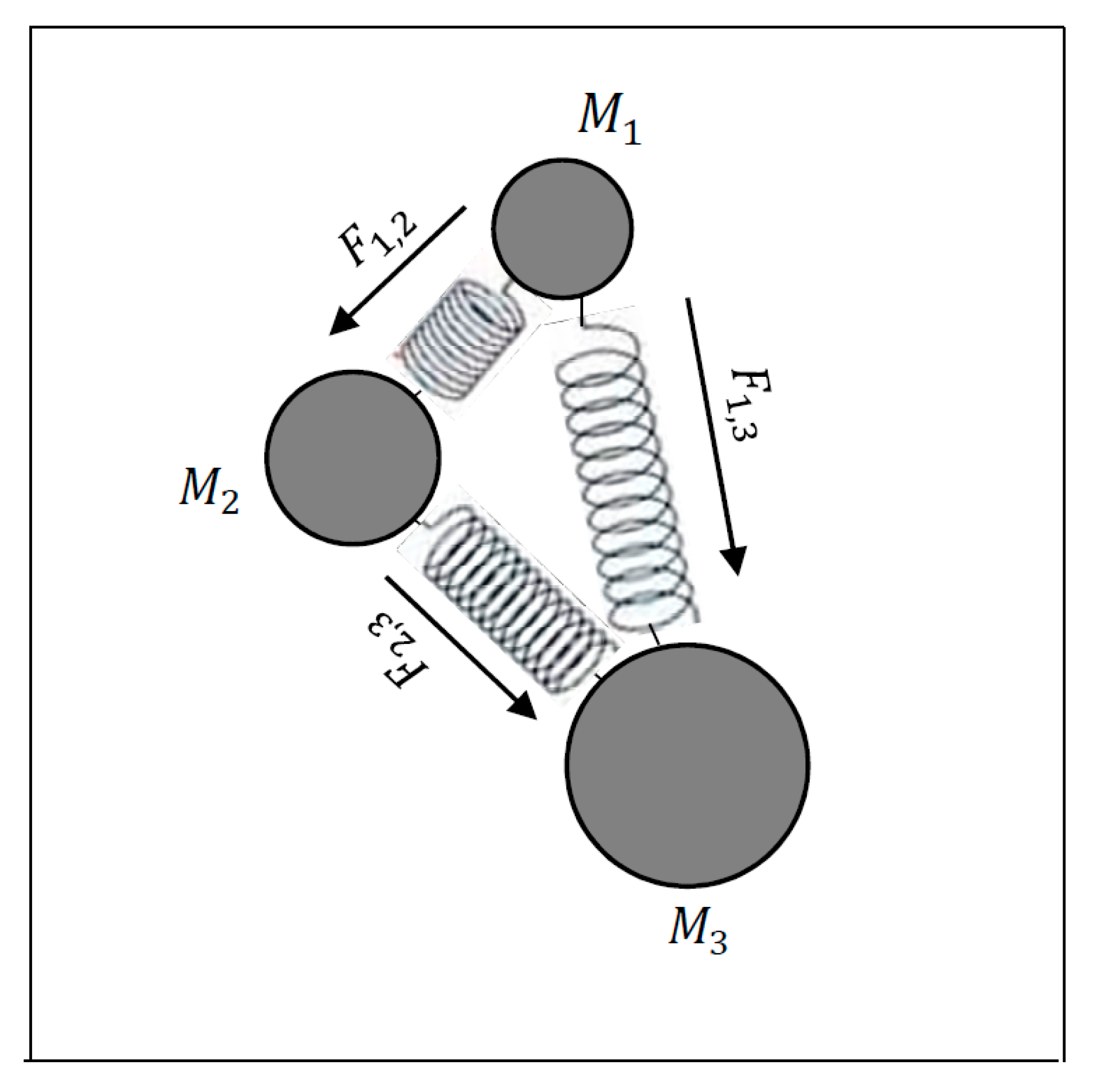
3. Spring Force Law
4. Spring Search Algorithm (SSA)
4.1. Setting the System, Determining Laws and Arranging Parameters
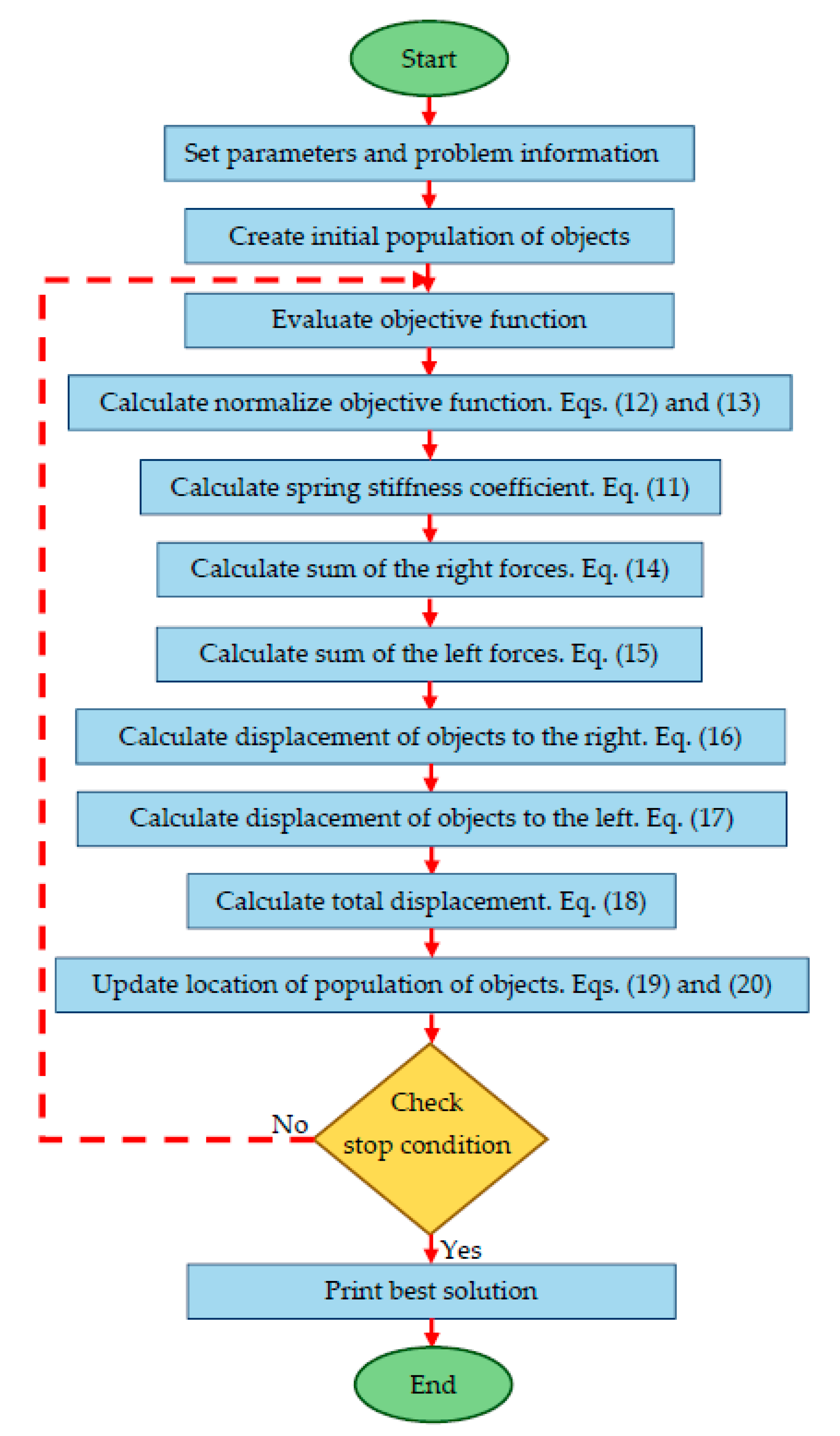
4.2. Time Passing and Parameters Updating
- 1-
- Start
- 2-
- Determine the system environment and the problem information
- 3-
- Create the initial population of objects
- 4-
- Evaluate and normalize fitness function or objective function
- 5-
- Update parameter K
- 6-
- Formulate the spring force and the laws of motion for each object
- 7-
- Compute object displacement quantities
- 8-
- Update object locations
- 9-
- Repeat steps 4 through 8 until the stop condition is satisfied
- 10-
- Print best solution
- 11-
- End
5. Properties of the Proposed SSA
6. Exploration and Exploitation in SSA
7. Experimental Results and Discussion
7.1. Benchmark Test Functions
7.2. Algorithms Used for Comparison
| Parameter definition |
| 1: GA 2: Population size N = 80 3: Crossover 0.9 4: Mutation 0.05 5: PSO 6: Swarm size S = 50 7: Inertia weight decreases linearly from 0.9 to 0.4 8: C1(individual-best acceleration factor) increases linearly from 0.5 to 2.5 9: C2(global-best acceleration factor) decreases linearly from 2.5 to 0.5 10: GSA 11: Objects number N = 50 12: Acceleration coefficient (a = 20) 13: Initial gravitational constant (G0 = 100) 14: TLBO 15: Swarm size S = 50 16: GOA 17: Search Agents N = 100 18: 19: 20: l = 1.5 and f = 0.5 21: GWO 22: Wolves number = 50 23: a variable decreases linearly from 2 to 0 24: SHO 25: Search Agents N = 80 26: M Constant 27: Control Parameter (h) 28: EPO 29: Search Agents N = 80 30: Temperature Profile 31: A Constant 32: Function S() 33: Parameter M = 2 34: Parameter f 35: Parameter l |
7.2.1. Evaluation of Unimodal Test Function with High Dimensions
7.2.2. Evaluation of Multimodal Test Functions with High Dimensions
7.2.3. Evaluation of Multimodal Test Functions with Low Dimensions
7.2.4. Evaluation of CEC 2015 Test Functions
8. SSA for Engineering Design Problems
8.1. Pressure Vessel Design
8.2. Speed Reducer Design Problem
8.3. Welded Beam Design
8.4. Tension/Compression Spring Design Problem
8.5. Rolling Element Bearing Design Problem
9. Conclusions
Author Contributions
Funding
Conflicts of Interest
Abbreviations
| Acronym | Definition |
| ABC | Artificial Bee Colony |
| ACROA | Artificial Chemical Reaction Optimization Algorithm |
| AFSA | Artificial Fish-Swarm Algorithm |
| BA | Bat-inspired Algorithm |
| BBO | Biogeography-Based Optimizer |
| BH | Black Hole |
| BOSA | Binary Orientation Search Algorithm |
| BBBC | Big-Bang Big-Crunch |
| CFO | Central Force Optimization |
| CS | Cuckoo Search |
| CSO | Curved Space Optimization |
| CSS | Charged System Search |
| DGO | Darts Game Optimizer |
| DPO | Dolphin Partner Optimization |
| DGO | Dice Game Optimizer |
| DE | Differential Evolution |
| DTO | Donkey Theorem Optimization |
| EP | Evolutionary Programming |
| ES | Evolution Strategy |
| EPO | Emperor Penguin Optimizer |
| FA | Firefly Algorithm |
| FOA | Following Optimization Algorithm |
| FGBO | Football Game Based Optimization |
| GP | Genetic Programming |
| GO | Group Optimization |
| GOA | Grasshopper Optimization Algorithm |
| GSA | Gravitational Search Algorithm |
| GbSA | Galaxy-based Search Algorithm |
| GWO | Grey Wolf Optimizer |
| HOGO | Hide Objects Game Optimization |
| HS | Hunting Search |
| MFO | Moth-flame Optimization Algorithm |
| MS | Monkey Search |
| OSA | Orientation Search Algorithm |
| PSO | Particle Swarm Optimization |
| RSO | Rat Swarm Optimizer |
| RO | Ray Optimization |
| SHO | Spotted Hyena Optimizer |
| SGO | Shell Game Optimization |
| SWOA | Small World Optimization Algorithm |
| WOA | Whale Optimization Algorithm |
References
- Cortés-Toro, E.M.; Crawford, B.; Gómez-Pulido, J.A.; Soto, R.; Lanza-Gutiérrez, J.M. A new metaheuristic inspired by the vapour-liquid equilibrium for continuous optimization. Appl. Sci. 2018, 8, 2080. [Google Scholar] [CrossRef]
- Pelusi, D.; Mascella, R.; Tallini, L. A fuzzy gravitational search algorithm to design optimal IIR filters. Energies 2018, 11, 736. [Google Scholar] [CrossRef]
- Díaz, P.; Pérez-Cisneros, M.; Cuevas, E.; Avalos, O.; Gálvez, J.; Hinojosa, S.; Zaldivar, D. An improved crow search algorithm applied to energy problems. Energies 2018, 11, 571. [Google Scholar] [CrossRef]
- Chiu, C.-Y.; Shih, P.-C.; Li, X. A dynamic adjusting novel global harmony search for continuous optimization problems. Symmetry 2018, 10, 337. [Google Scholar] [CrossRef]
- Sengupta, S.; Basak, S.; Peters, R.A. Particle Swarm Optimization: A survey of historical and recent developments with hybridization perspectives. Mach. Learn. Knowl. Extr. 2019, 1, 157–191. [Google Scholar] [CrossRef]
- Stripling, E.; Broucke, S.V.; Antonio, K.; Baesens, B.; Snoeck, M. Profit maximizing logistic model for customer churn prediction using genetic algorithms. Swarm Evol. Comput. 2018, 40, 116–130. [Google Scholar] [CrossRef]
- Antonov, I.V.; Mazurov, E.; Borodovsky, M.; Medvedeva, Y.A. Prediction of lncRNAs and their interactions with nucleic acids: Benchmarking bioinformatics tools. Brief. Bioinform. 2019, 20, 551–564. [Google Scholar] [CrossRef]
- Djenouri, Y.; Belhadi, A.; Belkebir, R. Bees swarm optimization guided by data mining techniques for document information retrieval. Expert Syst. Appl. 2018, 94, 126–136. [Google Scholar] [CrossRef]
- Artrith, N.; Urban, A.; Ceder, G. Constructing first-principles phase diagrams of amorphous Li x Si using machine-learning-assisted sampling with an evolutionary algorithm. J. Chem. Phys. 2018, 148, 241711. [Google Scholar] [CrossRef]
- Dehghani, M.; Montazeri, Z.; Malik, O. Energy commitment: A planning of energy carrier based on energy consumption. Электрoтехника и электрoмеханика 2019, 4, 69–72. [Google Scholar] [CrossRef]
- Ehsanifar, A.; Dehghani, M.; Allahbakhshi, M. Calculating the leakage inductance for transformer inter-turn fault detection using finite element method. In Proceedings of the 2017 Iranian Conference on Electrical Engineering (ICEE), Tehran, Iran, 2–4 May 2017; pp. 1372–1377. [Google Scholar]
- Dehghani, M.; Montazeri, Z.; Malik, O. Optimal sizing and placement of capacitor banks and distributed generation in distribution systems using spring search algorithm. Int. J. Emerg. Electr. Power Syst. 2020, 21. [Google Scholar] [CrossRef]
- Dehghani, M.; Montazeri, Z.; Malik, O.P.; Al-Haddad, K.; Guerrero, J.M.; Dhiman, G. A New Methodology Called Dice Game Optimizer for Capacitor Placement in Distribution Systems. Электрoтехника и электрoмеханика 2020, 1, 61–64. [Google Scholar] [CrossRef]
- Dehbozorgi, S.; Ehsanifar, A.; Montazeri, Z.; Dehghani, M.; Seifi, A. Line loss reduction and voltage profile improvement in radial distribution networks using battery energy storage system. In Proceedings of the 2017 IEEE 4th International Conference on Knowledge-Based Engineering and Innovation (KBEI), Tehran, Iran, 22 December 2017; pp. 215–219. [Google Scholar]
- Montazeri, Z.; Niknam, T. Optimal utilization of electrical energy from power plants based on final energy consumption using gravitational search algorithm. Электрoтехника и электрoмеханика 2018, 4, 70–73. [Google Scholar] [CrossRef]
- Dehghani, M.; Mardaneh, M.; Montazeri, Z.; Ehsanifar, A.; Ebadi, M.; Grechko, O. Spring search algorithm for simultaneous placement of distributed generation and capacitors. Электрoтехника и электрoмеханика 2018, 6, 68–73. [Google Scholar] [CrossRef]
- Dehghani, M.; Montazeri, Z.; Ehsanifar, A.; Seifi, A.; Ebadi, M.; Grechko, O. Planning of energy carriers based on final energy consumption using dynamic programming and particle swarm optimization. Электрoтехника и электрoмеханика 2018, 5, 62–71. [Google Scholar] [CrossRef]
- Montazeri, Z.; Niknam, T. Energy carriers management based on energy consumption. In Proceedings of the2017 IEEE 4th International Conference on Knowledge-Based Engineering and Innovation (KBEI), Tehran, Iran, 22 December 2017; pp. 539–543. [Google Scholar]
- Mirjalili, S. Genetic Algorithm. In Evolutionary Algorithms and Neural Networks; Springer: Berlin/Heidelberg, Germany, 2019; pp. 43–55. [Google Scholar]
- Kirkpatrick, S.; Gelatt, C.D.; Vecchi, M.P. Optimization by simulated annealing. Science 1983, 220, 671–680. [Google Scholar] [CrossRef]
- Farmer, J.D.; Packard, N.H.; Perelson, A.S. The immune system, adaptation, and machine learning. Phys. D Nonlinear Phenom. 1986, 22, 187–204. [Google Scholar] [CrossRef]
- Mirjalili, S. Ant Colony Optimisation. In Evolutionary Algorithms and Neural Networks; Springer: Berlin/Heidelberg, Germany, 2019; pp. 33–42. [Google Scholar]
- Mirjalili, S. Particle Swarm Optimisation. In Evolutionary Algorithms and Neural Networks; Springer: Berlin/Heidelberg, Germany, 2019; pp. 15–31. [Google Scholar]
- Dehghani, M.; Montazeri, Z.; Dehghani, A.; Seifi, A. Spring search algorithm: A new meta-heuristic optimization algorithm inspired by Hooke’s law. In Proceedings of the 2017 IEEE 4th International Conference on Knowledge-Based Engineering and Innovation (KBEI), Tehran, Iran, 22 December 2017; pp. 210–214. [Google Scholar]
- Mirjalili, S. Biogeography-Based Optimisation. In Evolutionary Algorithms and Neural Networks; Springer: Berlin/Heidelberg, Germany, 2019; pp. 57–72. [Google Scholar]
- Gigerenzer, G.; Gaissmaier, W. Heuristic decision making. Annu. Rev. Psychol. 2011, 62, 451–482. [Google Scholar] [CrossRef]
- Lim, S.M.; Leong, K.Y. A Brief Survey on Intelligent Swarm-Based Algorithms for Solving Optimization Problems. In Nature-inspired Methods for Stochastic, Robust and Dynamic Optimization; IntechOpen: London, UK, 2018. [Google Scholar]
- Kennedy, J.; Eberhart, R. Particle swarm optimization, proceeding of the IEEE International Conference on Neural Networks, Perth, Australia. IEEE Serv. Cent. Piscataway 1942, 1948, 1995. [Google Scholar]
- Yang, X.-S. Firefly algorithm, stochastic test functions and design optimization. arXiv 2010, arXiv:1003.1409. [Google Scholar]
- Mirjalili, S.; Lewis, A. The whale optimization algorithm. Adv. Eng. Softw. 2016, 95, 51–67. [Google Scholar] [CrossRef]
- Karaboga, D.; Basturk, B. Artificial bee colony (ABC) optimization algorithm for solving constrained optimization. In Problems, LNCS: Advances in Soft Computing: Foundations of Fuzzy Logic and Soft Computing; Springer: Berlin/Heidelberg, Germany, 2007. [Google Scholar]
- Yang, X.-S. A new metaheuristic bat-inspired algorithm. In Nature Inspired Cooperative Strategies for Optimization (NICSO 2010); Springer: Berlin/Heidelberg, Germany, 2010; pp. 65–74. [Google Scholar]
- Dhiman, G.; Kumar, V. Spotted hyena optimizer: A novel bio-inspired based metaheuristic technique for engineering applications. Adv. Eng. Softw. 2017, 114, 48–70. [Google Scholar] [CrossRef]
- Gandomi, A.H.; Yang, X.-S.; Alavi, A.H. Cuckoo search algorithm: A metaheuristic approach to solve structural optimization problems. Eng. Comput. 2013, 29, 17–35. [Google Scholar] [CrossRef]
- Mucherino, A.; Seref, O. Monkey search: A novel metaheuristic search for global optimization. AIP Conf. Proc. 2007, 953, 162–173. [Google Scholar]
- Dehghani, M.; Montazeri, Z.; Dehghani, A.; Malik, O.P. GO: Group Optimization. Gazi Univ. J. Sci. 2020, 33, 381–392. [Google Scholar] [CrossRef]
- Neshat, M.; Sepidnam, G.; Sargolzaei, M.; Toosi, A.N. Artificial fish swarm algorithm: A survey of the state-of-the-art, hybridization, combinatorial and indicative applications. Artif. Intell. Rev. 2014, 42, 965–997. [Google Scholar] [CrossRef]
- Oftadeh, R.; Mahjoob, M.; Shariatpanahi, M. A novel meta-heuristic optimization algorithm inspired by group hunting of animals: Hunting search. Comput. Math. Appl. 2010, 60, 2087–2098. [Google Scholar] [CrossRef]
- Mirjalili, S. Moth-flame optimization algorithm: A novel nature-inspired heuristic paradigm. Knowl. Based Syst. 2015, 89, 228–249. [Google Scholar] [CrossRef]
- Shiqin, Y.; Jianjun, J.; Guangxing, Y. A dolphin partner optimization. In Proceedings of the Global Congress on Intelligent Systems, Xiamen, China, 19–21 May 2009; pp. 124–128. [Google Scholar]
- Dehghani, M.; Montazeri, Z.; Malik, O.P.; Ehsanifar, A.; Dehghani, A. OSA: Orientation Search Algorithm. Int. J. Ind. Electron. Control Optim. 2019, 2, 99–112. [Google Scholar]
- Dehghani, M.; Montazeri, Z.; Malik, O.P.; Dhiman, G.; Kumar, V. BOSA: Binary Orientation Search Algorithm. Int. J. Innov. Technol. Explor. Eng. (IJITEE) 2019, 9, 5306–5310. [Google Scholar]
- Dehghani, M.; Montazeri, Z.; Malik, O.P. DGO: Dice Game Optimizer. Gazi Univ. J. Sci. 2019, 32, 871–882. [Google Scholar] [CrossRef]
- Mohammad, D.; Zeinab, M.; Malik, O.P.; Givi, H.; Guerrero, J.M. Shell Game Optimization: A Novel Game-Based Algorithm. Int. J. Intell. Eng. Syst. 2020, 13, 246–255. [Google Scholar]
- Dehghani, M.; Montazeri, Z.; Saremi, S.; Dehghani, A.; Malik, O.P.; Al-Haddad, K.; Guerrero, J.M. HOGO: Hide Objects Game Optimization. Int. J. Intell. Eng. Syst. 2020, 13, 216–225. [Google Scholar] [CrossRef]
- Dehghani, M.; Mardaneh, M.; Malik, O.P.; NouraeiPour, S.M. DTO: Donkey Theorem Optimization. In Proceedings of the 2019 27th Iranian Conference on Electrical Engineering (ICEE), Yazd, Iran, 30 April–2 May 2019; pp. 1855–1859. [Google Scholar]
- Dehghani, M.; Mardaneh, M.; Malik, O. FOA: ‘Following’Optimization Algorithm for solving Power engineering optimization problems. J. Oper. Autom. Power Eng. 2020, 8, 57–64. [Google Scholar]
- Dhiman, G.; Garg, M.; Nagar, A.K.; Kumar, V.; Dehghani, M. A Novel Algorithm for Global Optimization: Rat Swarm Optimizer. J. Ambient Intell. Humaniz. Comput. 2020, 1, 1–6. [Google Scholar]
- Dehghani, M.; Montazeri, Z.; Givi, H.; Guerrero, J.M.; Dhiman, G. Darts Game Optimizer: A New Optimization Technique Based on Darts Game. Int. J. Intell. Eng. Syst. 2020, 13, 286–294. [Google Scholar]
- Dehghani, M.; Mardaneh, M.; Guerrero, J.M.; Malik, O.P.; Kumar, V. Football Game Based Optimization: An Application to Solve Energy Commitment Problem. Int. J. Intell. Eng. Syst. 2020, 13, 514–523. [Google Scholar] [CrossRef]
- Mirjalili, S.; Mirjalili, S.M.; Lewis, A. Grey wolf optimizer. Adv. Eng. Softw. 2014, 69, 46–61. [Google Scholar] [CrossRef]
- Saremi, S.; Mirjalili, S.; Lewis, A. Grasshopper optimisation algorithm: Theory and application. Adv. Eng. Softw. 2017, 105, 30–47. [Google Scholar] [CrossRef]
- Zhang, H.; Hui, Q. A Coupled Spring Forced Bat Searching Algorithm: Design, Analysis and Evaluation. In Proceedings of the 2020 American Control Conference (ACC), Denver, CO, USA, 1–3 July 2020; pp. 5016–5021. [Google Scholar]
- Wang, Z.-J.; Zhan, Z.-H.; Kwong, S.; Jin, H.; Zhang, J. Adaptive Granularity Learning Distributed Particle Swarm Optimization for Large-Scale Optimization. IEEE Trans. Cybern. 2020, 1–14. [Google Scholar] [CrossRef]
- Dehghani, M.; Montazeri, Z.; Dehghani, A.; Ramirez-Mendoza, R.A.; Samet, H.; Guerrero, J.M.; Dhiman, G. MLO: Multi Leader Optimizer. Int. J. Intell. Eng. Syst. 2020, 1, 1–11. [Google Scholar]
- Dehghani, M.; Mardaneh, M.; Guerrero, J.M.; Malik, O.P.; Ramirez-Mendoza, R.A.; Matas, J.; Vasquez, J.C.; Parra-Arroyo, L. A New “Doctor and Patient” Optimization Algorithm: An Application to Energy Commitment Problem. Appl. Sci. 2020, 10, 5791. [Google Scholar] [CrossRef]
- Dhiman, G.; Kumar, V. Emperor Penguin Optimizer: A Bio-inspired Algorithm for Engineering Problems. Knowl. Based Syst. 2018, 159, 20–50. [Google Scholar] [CrossRef]
- Karkalos, N.E.; Markopoulos, A.P.; Davim, J.P. Evolutionary-Based Methods. In Computational Methods for Application in Industry 4.0; Springer: Berlin/Heidelberg, Germany, 2019; pp. 11–31. [Google Scholar]
- Mirjalili, S. Introduction to Evolutionary Single-Objective Optimisation. In Evolutionary Algorithms and Neural Networks; Springer: Berlin/Heidelberg, Germany, 2019; pp. 3–14. [Google Scholar]
- Holland, J.H. Genetic Algorithms. Sci. Am. 1992, 267, 66–73. [Google Scholar] [CrossRef]
- Bageley, J. The Behavior of Adaptive Systems Which Employ Genetic and Correlation Algorithms. Ph.D. Thesis, University of Michigan, Ann Arbor, MI, USA, 1967. [Google Scholar]
- Bose, A.; Biswas, T.; Kuila, P. A Novel Genetic Algorithm Based Scheduling for Multi-core Systems. In Smart Innovations in Communication and Computational Sciences; Springer: Berlin/Heidelberg, Germany, 2019; pp. 45–54. [Google Scholar]
- Das, S.; Suganthan, P.N. Differential evolution: A survey of the state-of-the-art. IEEE Trans. Evol. Comput. 2011, 15, 4–31. [Google Scholar] [CrossRef]
- Storn, R.; Price, K. Differential Evolution—A Simple and Efficient Adaptive Scheme for Global Optimization over Continuous Spaces; ICSI: Berkeley, CA, USA, 1995. [Google Scholar]
- Chakraborty, U.K. Advances in Differential Evolution; Springer: Berlin/Heidelberg, Germany, 2008; Volume 143. [Google Scholar]
- Fogel, L.J.; Owens, A.J.; Walsh, M.J. Artificial Intelligence through Simulated Evolution; Wiley: New York, NY, USA, 1966. [Google Scholar]
- Simon, D. Biogeography-based optimization. IEEE Trans. Evol. Comput. 2008, 12, 702–713. [Google Scholar] [CrossRef]
- Deng, W.; Liu, H.; Xu, J.; Zhao, H.; Song, Y. An improved quantum-inspired differential evolution algorithm for deep belief network. IEEE Trans. Instrum. Meas. 2020. [Google Scholar] [CrossRef]
- Koza, J.R. Genetic programming as a means for programming computers by natural selection. Stat. Comput. 1994, 4, 87–112. [Google Scholar] [CrossRef]
- Beyer, H.-G.; Schwefel, H.-P. Evolution strategies—A comprehensive introduction. Nat. Comput. 2002, 1, 3–52. [Google Scholar] [CrossRef]
- Kirkpatrick, S.; Gelatt, C.D.; Vecchi, M.P. A heuristic algorithm and simulation approach to relative location of facilities. Optim. Simulated Annealing 1983, 220, 671–680. [Google Scholar]
- Rashedi, E.; Nezamabadi-Pour, H.; Saryazdi, S. GSA: A gravitational search algorithm. Inf. Sci. 2009, 179, 2232–2248. [Google Scholar] [CrossRef]
- Rashedi, E.; Rashedi, E.; Nezamabadi-pour, H. A comprehensive survey on gravitational search algorithm. Swarm Evol. Comput. 2018, 41, 141–158. [Google Scholar] [CrossRef]
- Kaveh, A.; Talatahari, S. A novel heuristic optimization method: Charged system search. Acta Mech. 2010, 213, 267–289. [Google Scholar] [CrossRef]
- Shah-Hosseini, H. Principal components analysis by the galaxy-based search algorithm: A novel metaheuristic for continuous optimisation. Int. J. Comput. Sci. Eng. 2011, 6, 132–140. [Google Scholar]
- Moghaddam, F.F.; Moghaddam, R.F.; Cheriet, M. Curved space optimization: A random search based on general relativity theory. arXiv 2012, arXiv:1208.2214. [Google Scholar]
- Kaveh, A.; Khayatazad, M. A new meta-heuristic method: Ray optimization. Comput. Struct. 2012, 112, 283–294. [Google Scholar] [CrossRef]
- Alatas, B. ACROA: Artificial chemical reaction optimization algorithm for global optimization. Expert Syst. Appl. 2011, 38, 13170–13180. [Google Scholar] [CrossRef]
- Du, H.; Wu, X.; Zhuang, J. Small-world optimization algorithm for function optimization. In International Conference on Natural Computation; Springer: Berlin/Heidelberg, Germany, 2006; pp. 264–273. [Google Scholar]
- Formato, R.A. Central force optimization: A new nature inspired computational framework for multidimensional search and optimization. In Nature Inspired Cooperative Strategies for Optimization (NICSO 2007); Springer: Berlin/Heidelberg, Germany, 2008; pp. 221–238. [Google Scholar]
- Hatamlou, A. Black hole: A new heuristic optimization approach for data clustering. Inf. Sci. 2013, 222, 175–184. [Google Scholar] [CrossRef]
- Erol, O.K.; Eksin, I. A new optimization method: Big bang–big crunch. Adv. Eng. Softw. 2006, 37, 106–111. [Google Scholar] [CrossRef]
- Halliday, D.; Resnick, R.; Walker, J. Fundamentals of Physics; John Wiley & Sons: Hoboken, NJ, USA, 2013. [Google Scholar]
- Eiben, A.E.; Schippers, C.A. On evolutionary exploration and exploitation. Fundam. Inform. 1998, 35, 35–50. [Google Scholar] [CrossRef]
- Yao, X.; Liu, Y.; Lin, G. Evolutionary programming made faster. IEEE Trans. Evol. Comput. 1999, 3, 82–102. [Google Scholar]
- Chen, Q.; Liu, B.; Zhang, Q.; Liang, J.; Suganthan, P.; Qu, B. Problem Definition and Evaluation Criteria for CEC 2015 Special Session and Competition on Bound Constrained Single-Objective Computationally Expensive Numerical Optimization; Technical Report; Computational Intelligence Laboratory, Zhengzhou University, China and Nanyang Technological University: Singapore, 2014. [Google Scholar]
- Tang, K.-S.; Man, K.-F.; Kwong, S.; He, Q. Genetic algorithms and their applications. IEEE Signal Process. Mag. 1996, 13, 22–37. [Google Scholar] [CrossRef]
- Sarzaeim, P.; Bozorg-Haddad, O.; Chu, X. Teaching-Learning-Based Optimization (TLBO) Algorithm. In Advanced Optimization by Nature-Inspired Algorithms; Springer: Berlin/Heidelberg, Germany, 2018; pp. 51–58. [Google Scholar]
- Kannan, B.; Kramer, S.N. An augmented Lagrange multiplier based method for mixed integer discrete continuous optimization and its applications to mechanical design. J. Mech. Des. 1994, 116, 405–411. [Google Scholar] [CrossRef]
- Gandomi, A.H.; Yang, X.-S. Benchmark problems in structural optimization. In Computational Optimization, Methods and Algorithms; Springer: Berlin/Heidelberg, Germany, 2011; pp. 259–281. [Google Scholar]
- Mezura-Montes, E.; Coello, C.A.C. Useful infeasible solutions in engineering optimization with evolutionary algorithms. In Mexican International Conference on Artificial Intelligence; Springer: Berlin/Heidelberg, Germany, 2005; pp. 652–662. [Google Scholar]
- Rao, B.R.; Tiwari, R. Optimum design of rolling element bearings using genetic algorithms. Mech. Mach. Theory 2007, 42, 233–250. [Google Scholar]


| GA | PSO | GSA | TLBO | GOA | GWO | SHO | EPO | SSA | ||
|---|---|---|---|---|---|---|---|---|---|---|
| F1 | Ave | 1.95 × 10⁻¹² | 4.98 × 10−09 | 1.16 × 10⁻¹⁶ | 3.55 × 10−02 | 2.81 × 10−01 | 7.86 × 10⁻¹⁰ | 4.61 × 10⁻²³ | 5.71 × 10⁻²⁸ | 6.74 × 10⁻³⁵ |
| std | 2.01 × 10⁻¹¹ | 1.40 × 10−08 | 6.10 × 10⁻¹⁷ | 1.06 × 10−01 | 1.11 × 10−01 | 8.11 × 10−09 | 7.37 × 10⁻²³ | 8.31 × 10⁻²⁹ | 9.17 × 10−36 | |
| F2 | Ave | 6.53 × 10⁻¹⁸ | 7.29 × 10−04 | 1.70 × 10−01 | 3.23 × 10−05 | 3.96 × 10−01 | 5.99 × 10⁻²⁰ | 1.20 × 10⁻³⁴ | 6.20 × 10−40 | 7.78 × 10−45 |
| std | 5.10 × 10⁻¹⁷ | 1.84 × 10−03 | 9.29 × 10−01 | 8.57 × 10−05 | 1.41 × 10−01 | 1.11 × 10⁻¹⁷ | 1.30 × 10⁻³⁴ | 3.32 × 10−40 | 3.48 × 10−45 | |
| F3 | Ave | 7.70 × 10⁻¹⁰ | 1.40 × 1001 | 4.16 × 1002 | 4.91 × 1003 | 4.31 × 1001 | 9.19 × 10−05 | 1.00 × 10⁻¹⁴ | 2.05 × 10⁻¹⁹ | 2.63 × 10⁻²⁵ |
| std | 7.36 × 10−09 | 7.13 × 1000 | 1.56 × 1002 | 3.89 × 1003 | 8.97 × 1000 | 6.16 × 10−04 | 4.10 × 10⁻¹⁴ | 9.17 × 10⁻²⁰ | 9.83 × 10⁻²⁷ | |
| F4 | Ave | 9.17 × 1001 | 6.00 × 10−01 | 1.12 × 1000 | 1.87 × 1001 | 8.80 × 10−01 | 8.73 × 10−01 | 2.02 × 10⁻¹⁴ | 4.32 × 10⁻¹⁸ | 4.65 × 10⁻²⁶ |
| std | 5.67 × 1001 | 1.72 × 10−01 | 9.89 × 10−01 | 8.21 × 1000 | 2.50 × 10−01 | 1.19 × 10−01 | 2.43 × 10⁻¹⁴ | 3.98 × 10⁻¹⁹ | 4.68 × 10⁻²⁹ | |
| F5 | Ave | 5.57 × 1002 | 4.93 × 1001 | 3.85 × 1001 | 7.37 × 1002 | 1.18 × 1002 | 8.91 × 1002 | 2.79 × 1001 | 5.07 × 1000 | 5.41 × 10−01 |
| std | 4.16 × 1001 | 3.89 × 1001 | 3.47 × 1001 | 1.98 × 1003 | 1.43 × 1002 | 2.97 × 1002 | 1.84 × 1000 | 4.90 × 10−01 | 5.05 × 10−02 | |
| F6 | Ave | 3.15 × 10−01 | 9.23 × 10−09 | 1.08 × 10⁻¹⁶ | 4.88 × 1000 | 3.15 × 10−01 | 8.18 × 10⁻¹⁷ | 6.58 × 10−01 | 7.01 × 10⁻¹⁹ | 8.03 × 10⁻²⁴ |
| std | 9.98 × 10−02 | 1.78 × 10−08 | 4.00 × 10⁻¹⁷ | 9.75 × 10−01 | 9.98 × 10−02 | 1.70 × 10⁻¹⁸ | 3.38 × 10−01 | 4.39 × 10⁻²⁰ | 5.22 × 10⁻²⁶ | |
| F7 | Ave | 6.79 × 10−04 | 6.92 × 10−02 | 7.68 × 10−01 | 3.88 × 10−02 | 2.02 × 10−02 | 5.37 × 10−01 | 7.80 × 10−04 | 2.71 × 10−05 | 3.33 × 10−08 |
| std | 3.29 × 10−03 | 2.87 × 10−02 | 2.77 × 1000 | 5.79 × 10−02 | 7.43 × 10−03 | 1.89 × 10−01 | 3.85 × 10−04 | 9.26 × 10−06 | 1.18 × 10−06 | |
| GA | PSO | GSA | TLBO | GOA | GWO | SHO | EPO | SSA | ||
|---|---|---|---|---|---|---|---|---|---|---|
| F8 | Ave | −5.11 × 1002 | −5.01 × 1002 | −2.75 × 1002 | −3.81 × 1002 | −6.92 × 1002 | −4.69 × 1001 | −6.14 × 1002 | −8.76 × 1002 | −1.2 × 1004 |
| std | 4.37 × 1001 | 4.28 × 1001 | 5.72 × 1001 | 2.83 × 1001 | 9.19 × 1001 | 3.94 × 1001 | 9.32 × 1001 | 5.92 × 1001 | 9.14 × 10⁻¹² | |
| F9 | Ave | 1.23 × 10−01 | 1.20 × 10−01 | 3.35 × 1001 | 2.23 × 1001 | 1.01 × 1002 | 4.85 × 10−02 | 4.34 × 10−01 | 6.90 × 10−01 | 8.76 × 10−04 |
| std | 4.11 × 1001 | 4.01 × 1001 | 1.19 × 1001 | 3.25 × 1001 | 1.89 × 1001 | 3.91 × 1001 | 1.66 × 1000 | 4.81 × 10−01 | 4.85 × 10−02 | |
| F10 | Ave | 5.31 × 10⁻¹¹ | 5.20 × 10⁻¹¹ | 8.25 × 10−09 | 1.55 × 1001 | 1.15 × 1000 | 2.83 × 10−08 | 1.63 × 10⁻¹⁴ | 8.03 × 10⁻¹⁶ | 8.04 × 10⁻²⁰ |
| std | 1.11 × 10⁻¹⁰ | 1.08 × 10⁻¹⁰ | 1.90 × 10−09 | 8.11 × 1000 | 7.87 × 10−01 | 4.34 × 10−07 | 3.14 × 10⁻¹⁵ | 2.74 × 10⁻¹⁴ | 3.34 × 10⁻¹⁸ | |
| F11 | Ave | 3.31 × 10−06 | 3.24 × 10−06 | 8.19 × 1000 | 3.01 × 10−01 | 5.74 × 10−01 | 2.49 × 10−05 | 2.29 × 10−03 | 4.20 × 10−05 | 4.23 × 10⁻¹⁰ |
| std | 4.23 × 10−05 | 4.11 × 10−05 | 3.70 × 1000 | 2.89 × 10−01 | 1.12 × 10−01 | 1.34 × 10−04 | 5.24 × 10−03 | 4.73 × 10−04 | 5.11 × 10−07 | |
| F12 | Ave | 9.16 × 10−08 | 8.93 × 10−08 | 2.65 × 10−01 | 5.21 × 1001 | 1.27 × 1000 | 1.34 × 10−05 | 3.93 × 10−02 | 5.09 × 10−03 | 6.33 × 10−05 |
| std | 4.88 × 10−07 | 4.77 × 10−07 | 3.14 × 10−01 | 2.47 × 1002 | 1.02 × 1000 | 6.23 × 10−04 | 2.42 × 10−02 | 3.75 × 10−03 | 4.71 × 10−04 | |
| F13 | Ave | 6.39 × 10−02 | 6.26 × 10−02 | 5.73 × 10⁻³² | 2.81 × 1002 | 6.60 × 10−02 | 9.94 × 10−08 | 4.75 × 10−01 | 1.25 × 10−08 | 0.00 × 1000 |
| std | 4.49 × 10−02 | 4.39 × 10−02 | 8.95 × 10⁻³² | 8.63 × 1002 | 4.33 × 10−02 | 2.61 × 10−07 | 2.38 × 10−01 | 2.61 × 10−07 | 0.00 × 1000 | |
| GA | PSO | GSA | TLBO | GOA | GWO | SHO | EPO | SSA | ||
|---|---|---|---|---|---|---|---|---|---|---|
| F14 | Ave | 4.39 × 1000 | 2.77 × 1000 | 3.61 × 1000 | 6.79 × 1000 | 9.98 × 1001 | 1.26 × 1000 | 3.71 × 1000 | 1.08 × 1000 | 9.98 × 10−01 |
| std | 4.41 × 10−02 | 2.32 × 1000 | 2.96 × 1000 | 1.12 × 1000 | 9.14 × 10⁻¹ | 6.86 × 10−01 | 3.86 × 1000 | 4.11 × 10−02 | 7.64 × 10⁻¹² | |
| F15 | Ave | 7.36 × 10−02 | 9.09 × 10−03 | 6.84 × 10−02 | 5.15 × 10−02 | 7.15 × 10−02 | 1.01 × 10−02 | 3.66 × 10−02 | 8.21 × 10−03 | 3.3 × 10−04 |
| std | 2.39 × 10−03 | 2.38 × 10−03 | 7.37 × 10−02 | 3.45 × 10−03 | 1.26 × 10−01 | 3.75 × 10−03 | 7.60 × 10−02 | 4.09 × 10−03 | 1.25 × 10−05 | |
| F16 | Ave | −1.02 × 1000 | −1.02 × 1000 | −1.02 × 1000 | −1.01 × 1000 | −1.02 × 1000 | −1.02 × 1000 | −1.02 × 1000 | −1.02 × 1000 | −1.03 × 1000 |
| std | 4.19 × 10−07 | 0.00 × 1000 | 0.00 × 1000 | 3.64 × 10−08 | 4.74 × 10−08 | 3.23 × 10−05 | 7.02 × 10−09 | 9.80 × 10−07 | 5.12 × 10⁻¹⁰ | |
| F17 | Ave | 3.98 × 10−01 | 3.98 × 10−01 | 3.98 × 10−01 | 3.98 × 10−01 | 3.98 × 10−01 | 3.98 × 10−01 | 3.98 × 10−01 | 3.98 × 10−01 | 3.98 × 10−01 |
| std | 3.71 × 10⁻¹⁷ | 9.03 × 10⁻¹⁶ | 1.13 × 10⁻¹⁶ | 9.45 × 10⁻¹⁵ | 1.15 × 10−07 | 7.61 × 10−04 | 7.00 × 10−07 | 5.39 × 10−05 | 4.56 × 10⁻²¹ | |
| F18 | Ave | 3.00 × 1000 | 3.00 × 1000 | 3.00 × 1000 | 3.00 × 1000 | 3.00 × 1000 | 3.00 × 1000 | 3.00 × 1000 | 3.00 × 1000 | 3.00 × 1000 |
| std | 6.33 × 10−07 | 6.59 × 10−05 | 3.24 × 10−02 | 1.94 × 10⁻¹⁰ | 1.48 × 1001 | 2.25 × 10−05 | 7.16 × 10−06 | 1.15 × 10−08 | 1.15 × 10⁻¹⁸ | |
| F19 | Ave | −3.81 × 1000 | −3.80 × 1000 | −3.86 × 1000 | −3.73 × 1000 | −3.77 × 1000 | −3.75 × 1000 | −3.84 × 1000 | −3.86 × 1000 | −3.86 × 1000 |
| std | 4.37 × 10⁻¹⁰ | 3.37 × 10⁻¹⁵ | 4.15 × 10−01 | 9.69 × 10−04 | 3.53 × 10−07 | 2.55 × 10−03 | 1.57 × 10−03 | 6.50 × 10−07 | 5.61 × 10⁻¹⁰ | |
| F20 | Ave | −2.39 × 1000 | −3.32 × 1000 | −1.47 × 1000 | −2.17 × 1000 | −3.23 × 1000 | −2.84 × 1000 | −3.27 × 1000 | −2.81 × 1000 | −3.31 × 1000 |
| std | 4.37 × 10−01 | 2.66 × 10−01 | 5.32 × 10−01 | 1.64 × 10−01 | 5.37 × 10−02 | 3.71 × 10−01 | 7.27 × 10−02 | 7.11 × 10−01 | 4.29 × 10−05 | |
| F21 | Ave | −5.19 × 1000 | −7.54 × 1000 | −4570 | −7.33 × 1000 | −7.38 × 1000 | −2.28 × 1000 | −9.65 × 1000 | −8.07 × 1000 | −10.15 × 1000 |
| std | 2.34 × 1000 | 2.77 × 1000 | 1.30 × 1000 | 1.29 × 1000 | 2.91 × 1000 | 1.80 × 1000 | 1.54 × 1000 | 2.29 × 1000 | 1.25 × 10−02 | |
| F22 | Ave | −2.97 × 1000 | −8.55 × 1000 | −6.58 × 1000 | −1.00 × 1000 | −8.50 × 1000 | −3.99 × 1000 | −1.04 × 1000 | −10.01 × 1000 | −10.40 × 1000 |
| std | 1.37 × 10−02 | 3.08 × 1000 | 2.64 × 1000 | 2.89 × 10−04 | 3.02 × 1000 | 1.99 × 1000 | 2.73 × 10−04 | 3.97 × 10−02 | 3.65 × 10−07 | |
| F23 | Ave | −3.10 × 1000 | −9.19 × 1000 | −9.37 × 1000 | −2.46 × 1000 | −8.41 × 1000 | −4.49 × 1000 | −1.05 × 1001 | −3.41 × 1000 | −10.53 × 1000 |
| std | 2.37 × 1000 | 2.52 × 1000 | 2.75 × 1000 | 1.19 × 1000 | 3.13 × 1000 | 1.96 × 1000 | 1.81 × 10−04 | 1.11 × 10−02 | 5.26 × 10−06 | |
| GA | PSO | GSA | TLBO | GOA | GWO | SHO | EPO | SSA | ||
|---|---|---|---|---|---|---|---|---|---|---|
| Cec-1 | Ave | 8.89 × 1006 | 3.20 × 1007 | 7.65 × 1006 | 1.47 × 1006 | 4.37 × 1005 | 2.02 × 1006 | 2.28 × 1006 | 6.06 × 1005 | 1.50 × 1005 |
| std | 6.95 × 1006 | 8.37 × 1006 | 3.07 × 1006 | 2.63 × 1006 | 4.73 × 1005 | 2.08 × 1006 | 2.18 × 1006 | 5.02 × 1005 | 1.21 × 1005 | |
| Cec-2 | Ave | 2.97 × 1005 | 6.58 × 1003 | 7.33 × 1008 | 1.97 × 1004 | 9.41 × 1003 | 5.65 × 1006 | 3.13 × 1005 | 1.43 × 1004 | 4.40 × 1003 |
| std | 2.85 × 1003 | 1.09 × 1003 | 2.33 × 1008 | 1.46 × 1004 | 1.08 × 1004 | 6.03 × 1006 | 4.19 × 1005 | 1.03 × 1004 | 1.34 × 1008 | |
| Cec-3 | Ave | 3.20 × 1002 | 3.20 × 1002 | 3.20 × 1002 | 3.20 × 1002 | 3.20 × 1002 | 3.20 × 1002 | 3.20 × 1002 | 3.20 × 1002 | 3.20 × 1002 |
| std | 2.78 × 10−02 | 1.11 × 10−05 | 7.53 × 10−02 | 3.19 × 10−02 | 9.14 × 10−02 | 8.61 × 10−02 | 7.08 × 10−02 | 3.76 × 10−02 | 1.16 × 10−06 | |
| Cec-4 | Ave | 6.99 × 1002 | 4.39 × 1002 | 4.42 × 1002 | 4.18 × 1002 | 4.26 × 1002 | 4.09 × 1002 | 4.16 × 1002 | 4.11 × 1002 | 4.04 × 1002 |
| std | 6.43 × 1000 | 7.25 × 1000 | 7.72 × 1000 | 1.03 × 1001 | 1.17 × 1001 | 3.96 × 1000 | 1.03 × 1001 | 1.71 × 1001 | 5.61 × 1000 | |
| Cec-5 | Ave | 1.26 × 1003 | 1.75 × 1003 | 1.76 × 1003 | 1.09 × 1003 | 1.33 × 1003 | 8.65 × 1002 | 9.20 × 1002 | 9.13 × 1002 | 9.81 × 1002 |
| std | 1.86 × 1002 | 2.79 × 1002 | 2.30 × 1002 | 2.81 × 1002 | 3.45 × 1002 | 2.16 × 1002 | 1.78 × 1002 | 1.85 × 1002 | 1.06 × 1002 | |
| Cec-6 | Ave | 2.91 × 1005 | 3.91 × 1006 | 2.30 × 1004 | 3.82 × 1003 | 7.35 × 1003 | 1.86 × 1003 | 2.26 × 1004 | 1.29 × 1004 | 1.05 × 1003 |
| std | 1.67 × 1005 | 2.70 × 1006 | 2.41 × 1004 | 2.44 × 1003 | 3.82 × 1003 | 1.93 × 1003 | 2.45 × 1004 | 1.15 × 1004 | 1.05 × 1003 | |
| Cec-7 | Ave | 7.08 × 1002 | 7.08 × 1002 | 7.06 × 1002 | 7.02 × 1002 | 7.02 × 1002 | 7.02 × 1002 | 7.02 × 1002 | 7.02 × 1002 | 7.02 × 1002 |
| std | 2.97 × 1000 | 1.32 × 1000 | 9.07 × 10−01 | 9.40 × 10−01 | 1.10 × 1000 | 7.75 × 10−01 | 7.07 × 10−01 | 6.76 × 10−01 | 5.50 × 10−01 | |
| Cec-8 | Ave | 5.79 × 1004 | 6.07 × 1005 | 6.73 × 1003 | 2.58 × 1003 | 9.93 × 1003 | 3.43 × 1003 | 3.49 × 1003 | 1.86 × 1003 | 1.47 × 1003 |
| std | 2.76 × 1004 | 4.81 × 1005 | 3.36 × 1003 | 1.61 × 1003 | 8.74 × 1003 | 2.77 × 1003 | 2.04 × 1003 | 1.98 × 1003 | 1.34 × 1003 | |
| Cec-9 | Ave | 1.00 × 1003 | 1.00 × 1003 | 1.00 × 1003 | 1.00 × 1003 | 1.00 × 1003 | 1.00 × 1003 | 1.00 × 1003 | 1.00 × 1003 | 1.00 × 1003 |
| std | 3.97 × 1000 | 5.33 × 1000 | 9.79 × 10−01 | 5.29 × 10−02 | 2.20 × 10−01 | 7.23 × 10−02 | 1.28 × 10−01 | 1.43 × 10−01 | 1.51 × 10−03 | |
| Cec-10 | Ave | 4.13 × 1004 | 3.42 × 1005 | 9.91 × 1003 | 2.62 × 1003 | 8.39 × 1003 | 3.27 × 1003 | 4.00 × 1003 | 2.00 × 1003 | 1.23 × 1003 |
| std | 2.39 × 1004 | 1.74 × 1005 | 8.83 × 1003 | 1.78 × 1003 | 1.12 × 1004 | 1.84 × 1003 | 2.82 × 1003 | 2.73 × 1003 | 1.51 × 1003 | |
| Cec-11 | Ave | 1.36 × 1003 | 1.41 × 1003 | 1.35 × 1003 | 1.39 × 1003 | 1.37 × 1003 | 1.35 × 1003 | 1.40 × 1003 | 1.38 × 1003 | 1.35 × 1003 |
| std | 5.39 × 1001 | 7.73 × 1001 | 1.11 × 1002 | 5.42 × 1001 | 8.97 × 1001 | 1.12 × 1002 | 5.81 × 1001 | 2.42 × 1001 | 1.01 × 1001 | |
| Cec-12 | Ave | 1.31 × 1003 | 1.31 × 1003 | 1.31 × 1003 | 1.30 × 1003 | 1.30 × 1003 | 1.30 × 1003 | 1.30 × 1003 | 1.30 × 1003 | 1.30 × 1003 |
| std | 1.65 × 1000 | 2.05 × 1000 | 1.54 × 1000 | 8.07 × 10−01 | 9.14 × 10−01 | 6.94 × 10−01 | 6.69 × 10−01 | 7.89 × 10−01 | 1.50 × 10−01 | |
| Cec-13 | Ave | 1.35 × 1003 | 1.35 × 1003 | 1.30 × 1003 | 1.30 × 1003 | 1.30 × 1003 | 1.30 × 1003 | 1.30 × 1003 | 1.30 × 1003 | 1.30 × 1003 |
| std | 3.97 × 1001 | 4.70 × 1001 | 3.78 × 10−03 | 2.43 × 10−04 | 1.04 × 10−03 | 5.44 × 10−03 | 1.92 × 10−04 | 2.76 × 10−04 | 6.43 × 10−05 | |
| Cec-14 | Ave | 8.96 × 1003 | 9.30 × 1003 | 7.51 × 1003 | 7.34 × 1003 | 7.60 × 1003 | 7.10 × 1003 | 7.29 × 1003 | 4.25 × 1003 | 3.22 × 1003 |
| std | 6.32 × 1003 | 4.04 × 1002 | 1.52 × 1003 | 2.47 × 1003 | 1.29 × 1003 | 3.12 × 1003 | 2.45 × 1003 | 1.73 × 1003 | 2.12 × 1002 | |
| Cec-15 | Ave | 1.63 × 1003 | 1.64 × 1003 | 1.62 × 1003 | 1.60 × 1003 | 1.61 × 1003 | 1.60 × 1003 | 1.61 × 1003 | 1.60 × 1003 | 1.60 × 1003 |
| std | 3.67 × 1001 | 1.12 × 1001 | 3.64 × 1000 | 1.80 × 10−02 | 1.13 × 1001 | 2.66 × 1000 | 4.94 × 1000 | 3.76 × 1000 | 5.69 × 10−01 | |
| Algorithms | Optimum Variables | Optimum Cost | |||
|---|---|---|---|---|---|
| Ts | Th | R | L | ||
| SSA | 0.778099 | 0.383241 | 40.315121 | 200.00000 | 5880.0700 |
| EPO | 0.778210 | 0.384889 | 40.315040 | 200.00000 | 5885.5773 |
| SHO | 0.779035 | 0.384660 | 40.327793 | 199.65029 | 5889.3689 |
| GOA | 0.778961 | 0.384683 | 40.320913 | 200.00000 | 5891.3879 |
| GWO | 0.845719 | 0.418564 | 43.816270 | 156.38164 | 6011.5148 |
| TLBO | 0.817577 | 0.417932 | 41.74939 | 183.57270 | 6137.3724 |
| GSA | 1.085800 | 0.949614 | 49.345231 | 169.48741 | 11,550.2976 |
| PSO | 0.752362 | 0.399540 | 40.452514 | 198.00268 | 5890.3279 |
| GA | 1.099523 | 0.906579 | 44.456397 | 179.65887 | 6550.0230 |
| Algorithms | Best | Mean | Worst | Std. Dev. | Median |
|---|---|---|---|---|---|
| SSA | 5880.0700 | 5891.3099 | 024.341 | 5883.5153 | |
| EPO | 5885.5773 | 5887.4441 | 5892.3207 | 002.893 | 5886.2282 |
| SHO | 5889.3689 | 5891.5247 | 5894.6238 | 013.910 | 5890.6497 |
| GOA | 5891.3879 | 6531.5032 | 7394.5879 | 534.119 | 6416.1138 |
| GWO | 6011.5148 | 6477.3050 | 7250.9170 | 327.007 | 6397.4805 |
| TLBO | 6137.3724 | 6326.7606 | 6512.3541 | 126.609 | 6318.3179 |
| GSA | 11,550.2976 | 23,342.2909 | 33,226.2526 | 5790.625 | 24,010.0415 |
| PSO | 5890.3279 | 6264.0053 | 7005.7500 | 496.128 | 6112.6899 |
| GA | 6550.0230 | 6643.9870 | 8005.4397 | 657.523 | 7586.0085 |
| Algorithms | Optimum Variables | Optimum Cost | ||||||
|---|---|---|---|---|---|---|---|---|
| b | m | p | l1 | l2 | d1 | d2 | ||
| SSA | 3.50123 | 0.7 | 17 | 7.3 | 7.8 | 3.33421 | 5.26536 | 2994.2472 |
| EPO | 3.50159 | 0.7 | 17 | 7.3 | 7.8 | 3.35127 | 5.28874 | 2998.5507 |
| SHO | 3.506690 | 0.7 | 17 | 7.380933 | 7.815726 | 3.357847 | 5.286768 | 3001.288 |
| GOA | 3.500019 | 0.7 | 17 | 8.3 | 7.8 | 3.352412 | 5.286715 | 3005.763 |
| GWO | 3.508502 | 0.7 | 17 | 7.392843 | 7.816034 | 3.358073 | 5.286777 | 3002.928 |
| TLBO | 3.508755 | 0.7 | 17 | 7.3 | 7.8 | 3.461020 | 5.289213 | 3030.563 |
| GSA | 3.600000 | 0.7 | 17 | 8.3 | 7.8 | 3.369658 | 5.289224 | 3051.120 |
| PSO | 3.510253 | 0.7 | 17 | 8.35 | 7.8 | 3.362201 | 5.287723 | 3067.561 |
| GA | 3.520124 | 0.7 | 17 | 8.37 | 7.8 | 3.366970 | 5.288719 | 3029.002 |
| Algorithms | Best | Mean | Worst | Std. Dev. | Median |
|---|---|---|---|---|---|
| SSA | 2994.2472 | 2997.482 | 2999.092 | 1.78091 | 2996.318 |
| EPO | 2998.5507 | 2999.640 | 3003.889 | 1.93193 | 2999.187 |
| SHO | 3001.288 | 3005.845 | 3008.752 | 5.83794 | 3004.519 |
| GOA | 3005.763 | 3105.252 | 3211.174 | 79.6381 | 3105.252 |
| GWO | 3002.928 | 3028.841 | 3060.958 | 13.0186 | 3027.031 |
| TLBO | 3030.563 | 3065.917 | 3104.779 | 18.0742 | 3065.609 |
| GSA | 3051.120 | 3170.334 | 3363.873 | 92.5726 | 3156.752 |
| PSO | 3067.561 | 3186.523 | 3313.199 | 17.1186 | 3198.187 |
| GA | 3029.002 | 3295.329 | 3619.465 | 57.0235 | 3288.657 |
| Algorithms | Optimum Variables | Optimum Cost | |||
|---|---|---|---|---|---|
| h | l | t | b | ||
| SSA | 0.205411 | 3.472341 | 9.035215 | 0.201153 | 1.723589 |
| EPO | 0.205563 | 3.474846 | 9.035799 | 0.205811 | 1.725661 |
| SHO | 0.205678 | 3.475403 | 9.036964 | 0.206229 | 1.726995 |
| GOA | 0.197411 | 3.315061 | 10.00000 | 0.201395 | 1.820395 |
| GWO | 0.205611 | 3.472103 | 9.040931 | 0.205709 | 1.725472 |
| TLBO | 0.204695 | 3.536291 | 9.004290 | 0.210025 | 1.759173 |
| GSA | 0.147098 | 5.490744 | 10.00000 | 0.217725 | 2.172858 |
| PSO | 0.164171 | 4.032541 | 10.00000 | 0.223647 | 1.873971 |
| GA | 0.206487 | 3.635872 | 10.00000 | 0.203249 | 1.836250 |
| Algorithms | Best | Mean | Worst | Std. Dev. | Median |
|---|---|---|---|---|---|
| SSA | 1.723589 | 1.725124 | 1.727211 | 0.004325 | 1.724399 |
| EPO | 1.725661 | 1.725828 | 1.726064 | 0.000287 | 1.725787 |
| SHO | 1.726995 | 1.727128 | 1.727564 | 0.001157 | 1.727087 |
| GOA | 1.820395 | 2.230310 | 3.048231 | 0.324525 | 2.244663 |
| GWO | 1.725472 | 1.729680 | 1.741651 | 0.004866 | 1.727420 |
| TLBO | 1.759173 | 1.817657 | 1.873408 | 0.027543 | 1.820128 |
| GSA | 2.172858 | 2.544239 | 3.003657 | 0.255859 | 2.495114 |
| PSO | 1.873971 | 2.119240 | 2.320125 | 0.034820 | 2.097048 |
| GA | 1.836250 | 1.363527 | 2.035247 | 0.139485 | 1.9357485 |
| Algorithms | Optimum Variables | Optimum Cost | ||
|---|---|---|---|---|
| d | D | p | ||
| SSA | 0.051087 | 0.342908 | 12.0898 | 0.012656987 |
| EPO | 0.051144 | 0.343751 | 12.0955 | 0.012674000 |
| SHO | 0.050178 | 0.341541 | 12.07349 | 0.012678321 |
| GOA | 0.05000 | 0.310414 | 15.0000 | 0.013192580 |
| GWO | 0.05000 | 0.315956 | 14.22623 | 0.012816930 |
| TLBO | 0.050780 | 0.334779 | 12.72269 | 0.012709667 |
| GSA | 0.05000 | 0.317312 | 14.22867 | 0.012873881 |
| PSO | 0.05010 | 0.310111 | 14.0000 | 0.013036251 |
| GA | 0.05025 | 0.316351 | 15.23960 | 0.012776352 |
| Algorithms | Best | Mean | Worst | Std. Dev. | Median |
|---|---|---|---|---|---|
| SSA | 0.012656987 | 0.012678903 | 0.012667902 | 0.001021 | 0.012676002 |
| EPO | 0.012674000 | 0.012684106 | 0.012715185 | 0.000027 | 0.012687293 |
| SHO | 0.012678321 | 0.012697116 | 0.012720757 | 0.000041 | 0.012699686 |
| GOA | 0.013192580 | 0.014817181 | 0.017862507 | 0.002272 | 0.013192580 |
| GWO | 0.012816930 | 0.014464372 | 0.017839737 | 0.001622 | 0.014021237 |
| TLBO | 0.012709667 | 0.012839637 | 0.012998448 | 0.000078 | 0.012844664 |
| GSA | 0.012873881 | 0.013438871 | 0.014211731 | 0.000287 | 0.013367888 |
| PSO | 0.013036251 | 0.014036254 | 0.016251423 | 0.002073 | 0.013002365 |
| GA | 0.012776352 | 0.013069872 | 0.015214230 | 0.000375 | 0.012952142 |
| Algorithms | Optimum Variables | Opt. Cost | |||||||||
|---|---|---|---|---|---|---|---|---|---|---|---|
| Dm | Db | Z | fi | fo | KDmin | KDmax | ε | e | ζ | ||
| SSA | 125 | 21.41890 | 10.94113 | 0.515 | 0.515 | 0.4 | 0.7 | 0.3 | 0.02 | 0.6 | 85,067.983 |
| EPO | 125 | 21.40732 | 10.93268 | 0.515 | 0.515 | 0.4 | 0.7 | 0.3 | 0.02 | 0.6 | 85,054.532 |
| SHO | 125.6199 | 21.35129 | 10.98781 | 0.515 | 0.515 | 0.5 | 0.68807 | 0.300151 | 0.03254 | 0.62701 | 84,807.111 |
| GOA | 125 | 20.75388 | 11.17342 | 0.515 | 0.515000 | 0.5 | 0.61503 | 0.300000 | 0.05161 | 0.60000 | 81,691.202 |
| GWO | 125.6002 | 21.32250 | 10.97338 | 0.515 | 0.515000 | 0.5 | 0.68782 | 0.301348 | 0.03617 | 0.61061 | 84,491.266 |
| TLBO | 125 | 21.14834 | 10.96928 | 0.515 | 0.515 | 0.5 | 0.7 | 0.3 | 0.02778 | 0.62912 | 83,431.117 |
| GSA | 125 | 20.85417 | 11.14989 | 0.515 | 0.517746 | 0.5 | 0.61827 | 0.304068 | 0.02000 | 0.624638 | 82,276.941 |
| PSO | 125 | 20.77562 | 11.01247 | 0.515 | 0.515000 | 0.5 | 0.61397 | 0.300000 | 0.05004 | 0.610001 | 82,773.982 |
| GA | 125 | 20.87123 | 11.16697 | 0.515 | 0.516000 | 0.5 | 0.61951 | 0.301128 | 0.05024 | 0.614531 | 81,569.527 |
| Algorithms | Best | Mean | Worst | Std. Dev. | Median |
|---|---|---|---|---|---|
| SSA | 85,067.983 | 85,042.352 | 86,551.599 | 1877.09 | 85,056.095 |
| EPO | 85,054.532 | 85,024.858 | 85,853.876 | 0186.68 | 85,040.241 |
| SHO | 84,807.111 | 84,791.613 | 84,517.923 | 0137.186 | 84,960.147 |
| GOA | 81,691.202 | 50,435.017 | 32,761.546 | 13,962.150 | 42,287.581 |
| GWO | 84,491.266 | 84,353.685 | 84,100.834 | 0392.431 | 84,398.601 |
| TLBO | 83,431.117 | 81,005.232 | 77,992.482 | 1710.777 | 81,035.109 |
| GSA | 82,276.941 | 78,002.107 | 71,043.110 | 3119.904 | 78,398.853 |
| PSO | 82,773.982 | 81,198.753 | 80,687.239 | 1679.367 | 8439.728 |
| GA | 81,569.527 | 80,397.998 | 79,412.779 | 1756.902 | 8347.009 |
© 2020 by the authors. Licensee MDPI, Basel, Switzerland. This article is an open access article distributed under the terms and conditions of the Creative Commons Attribution (CC BY) license (http://creativecommons.org/licenses/by/4.0/).
Share and Cite
Dehghani, M.; Montazeri, Z.; Dhiman, G.; Malik, O.P.; Morales-Menendez, R.; Ramirez-Mendoza, R.A.; Dehghani, A.; Guerrero, J.M.; Parra-Arroyo, L. A Spring Search Algorithm Applied to Engineering Optimization Problems. Appl. Sci. 2020, 10, 6173. https://doi.org/10.3390/app10186173
Dehghani M, Montazeri Z, Dhiman G, Malik OP, Morales-Menendez R, Ramirez-Mendoza RA, Dehghani A, Guerrero JM, Parra-Arroyo L. A Spring Search Algorithm Applied to Engineering Optimization Problems. Applied Sciences. 2020; 10(18):6173. https://doi.org/10.3390/app10186173
Chicago/Turabian StyleDehghani, Mohammad, Zeinab Montazeri, Gaurav Dhiman, O. P. Malik, Ruben Morales-Menendez, Ricardo A. Ramirez-Mendoza, Ali Dehghani, Josep M. Guerrero, and Lizeth Parra-Arroyo. 2020. "A Spring Search Algorithm Applied to Engineering Optimization Problems" Applied Sciences 10, no. 18: 6173. https://doi.org/10.3390/app10186173
APA StyleDehghani, M., Montazeri, Z., Dhiman, G., Malik, O. P., Morales-Menendez, R., Ramirez-Mendoza, R. A., Dehghani, A., Guerrero, J. M., & Parra-Arroyo, L. (2020). A Spring Search Algorithm Applied to Engineering Optimization Problems. Applied Sciences, 10(18), 6173. https://doi.org/10.3390/app10186173