Article

A Detailed One-Dimensional Hydrodynamic and Kinetic Model for Sorption Enhanced Gasification

University of Stuttgart, Institute of Combustion and Power Plant Technology (IFK), Pfaffenwaldring 23, 70569 Stuttgart, Germany
*
Author to whom correspondence should be addressed.
Appl. Sci. 2020, 10(17), 6136; https://doi.org/10.3390/app10176136
Submission received: 21 July 2020 / Revised: 19 August 2020 / Accepted: 27 August 2020 / Published: 3 September 2020

Abstract

:
Increased installation of renewable electricity generators requires different technologies to compensate for the associated fast and high load gradients. In this work, sorption enhanced gasification (SEG) in a dual fluidized bed gasification system is considered as a promising and flexible technology for the tailored syngas production for use in chemical manufacturing or electricity generation. To study different operational strategies, as defined by gasification temperature or fuel input, a simulation model is developed. This model considers the hydrodynamics in a bubbling fluidized bed gasifier and the kinetics of gasification reactions and CO2 capture. The CO2 capture rate is defined by the number of carbonation/calcination cycles and the make-up of fresh limestone. A parametric study of the make-up flow rate (0.2, 6.6, and 15 kg/h) reveals its strong influence on the syngas composition, especially at low gasification temperatures (600–650 °C). Our results show good agreement with the experimental data of a 200 kW pilot plant, as demonstrated by deviations of syngas composition (5–34%), lower heating value (LHV) (5–7%), and M module (23–32%). Studying the fuel feeding rate (22–40 kg/h), an operational range with a good mixing of solids in the fluidized bed is identified. The achieved results are summarized in a reactor performance diagram, which gives the syngas power depending on the gasification temperature and the fuel feeding rate.

1. Introduction

Global greenhouse gas (GHG) emissions have been increasing exponentially for the past 60 years, mostly due to the use of oil, coal, and natural gas [1,2]. Hereby, CO2 is the major GHG, accounting for 65% of the total amount. Replacing the usage of fossil fuels in combustion or gasification processes with biomass enables the reduction of CO2 emissions.
Sorption enhanced gasification (SEG) has been considered a promising technology for tailored syngas production with in situ CO2 capture. The plant configuration of a SEG process is based on the conventional steam gasification process carried out in indirect heated (or allothermal) dual fluidized bed systems. This conventional steam gasification process uses an inert bed material as a heat carrier to deliver the heat for the endothermic gasification, enabling N2-free syngas with typical hydrogen content of 20–40 vol% (on a dry basis). The syngas of this process can be used for power and heat generation, and the technology has already been applied in a number of industrial-scale facilities with thermal power ranging from 2–20 MW [3,4,5]. Accordingly, a number of different models describing the steam gasification of biomass have been developed and published [6,7,8].
Gordillo and Belghit [9] developed a two-phase model for steam gasification of biomass char which considers hydrodynamic phenomena; however, pyrolysis was not included, which is an important step in the biomass gasification process. Agu et al. [10] proposed a detailed one-dimensional model for steam gasification in a bubbling fluidized bed, which considers a Lagrangian approach for solid fuel particles extending the often used assumption of a uniform distribution of fuel particles. In contrast to conventional steam gasification, the SEG uses a reactive bed material (e.g., limestone) as the heat carrier, which enables the in situ capture of CO2 in the gasifier. This CO2 capture affects gasification reactions and shifts hydrogen concentrations in the syngas up to 75 vol% (on a dry basis) [11]. Thus, SEG has been considered to be a suitable process for the synthesis of hydrogen, transport fuels, and chemicals [12,13]. Hereby, models are important in finding the best operation strategies for the gasifier, especially if the gasifier is part of a complex production path, including mass and energy integration. However, few models exist which have considered the CO2 sorption characteristics in fluidized bed reactors. Inayat et al. [14] and Sreejith et al. [15] used a detailed approach based on reaction kinetics, but hydrodynamics were not in focus. In the work of Hejazi et al. [16,17], a model to describe sorption enhanced gasification in a bubbling fluidized bed was presented. This model considers hydrodynamics in the fluidized bed, but evaluations of process parameter over reactor height were not included due to the assumption of a uniform temperature throughout the dense bed. Another comprehensive SEG model has been published by Pitkäoja et al. [18]. This model considers a transport disengaging height to describe the amount of reacting particles in the freeboard, which is important for the overall syngas composition. However, minor focus is placed on the bed activity, which depends (in a dual fluidized system) on the mean particle residence time, as well as the carbonation/calcination cycles. Considering the issues discussed above, we developed a detailed SEG model focusing on various key aspects, including (i) hydrodynamic features of the fluidized bed reactor and evaluation of the process parameters over reactor height; (ii) kinetic aspects of the steam gasification process; and (iii) reaction kinetics of CO2 capture through carbonation in the fluidized bed, as well as by elutriated particles in the freeboard. As deactivation of the sorbent is an important issue in a SEG process, a deactivation model is included in this work.

2. SEG Process Description and Model Development

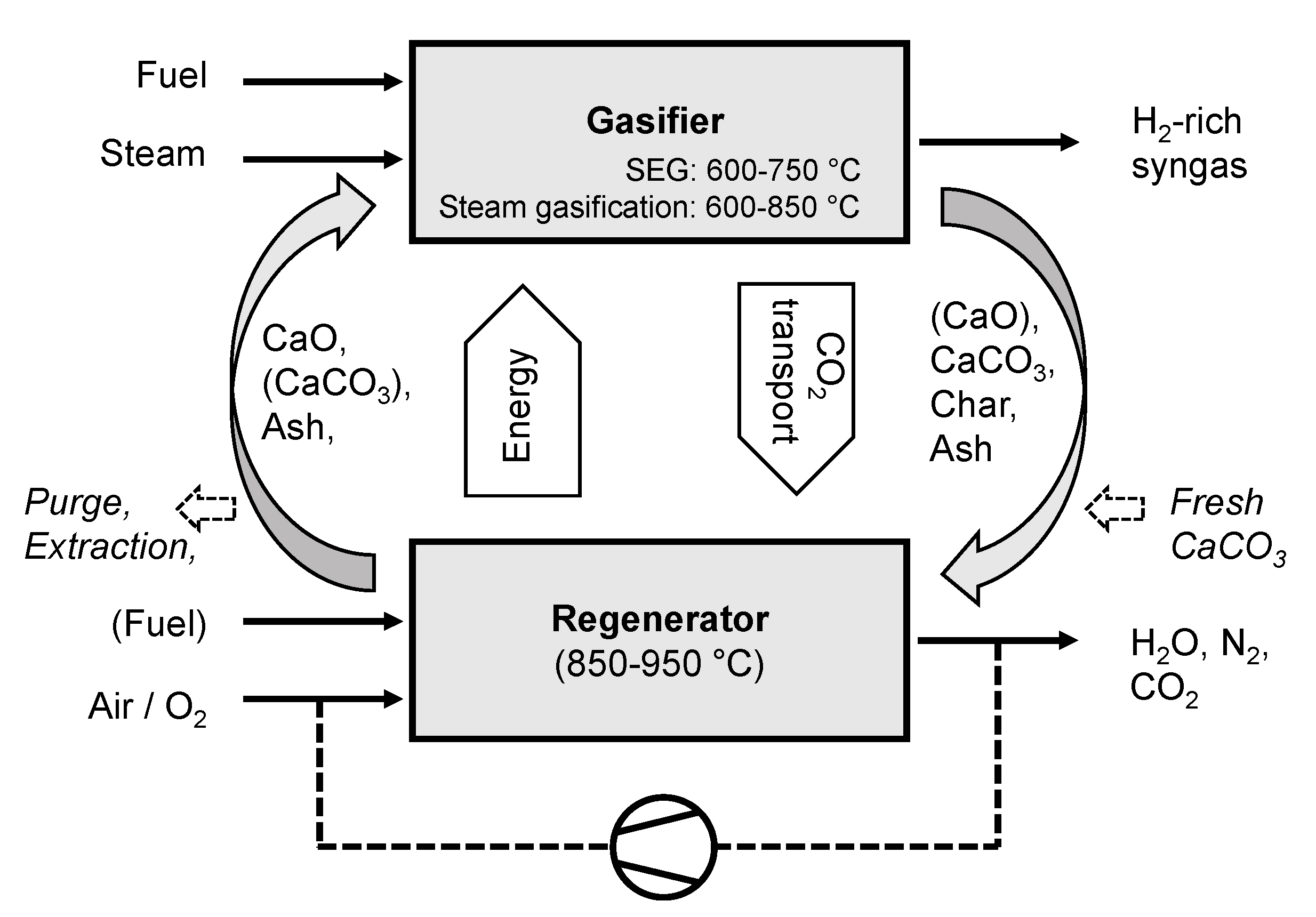
2.1. Description of the SEG Process

Based on availability of experimental data, atmospheric conditions were considered for sorption enhanced gasification (SEG). In this work, calcined limestone (CaO) was used as reactive bed material to capture CO2 from the syngas through the carbonation reaction (CaO + CO2 → CaCO3). This shifts gasification and water–gas shift reactions towards hydrogen production. The carbonation reaction proceeds until the equilibrium condition is reached, where the equilibrium depends on the temperature and CO2 partial pressure. Hence, the grade of CO2 capturing can be set by different operating conditions. Adjustment of syngas composition by selecting gasification temperature is a great advantage of the SEG process. Poboss [19] reported that there is a relatively high CO2 capture efficiency below 650 °C. For higher temperatures, the capture efficiency decreases rapidly. Based on the CO2 volume concentration in the wet syngas, the CO2 capture ceases at a temperature of 750–770 °C [19]. To a certain extent, operation above 750 °C and without CO2 separation can also be achieved with a dual fluidized bed system by increasing the solids circulation rate. The concept of SEG, with its two fluidized bed reactors, is illustrated in Figure 1. The energy needed for the endothermic gasification reactions in gasifier is supplied by the highly exothermic CaO carbonation reaction and by the sensible heat of circulating solids flowing from the regenerator (combustion reactor). This means if the temperature in the gasifier exceeds the range for carbonation reaction, the process is only driven by the temperature difference between regenerator and gasifier. However, the temperature of the regenerator cannot be set arbitrarily high since otherwise sintering of CaO will increasingly occur, resulting in a loss of activity [20]. To avoid sintering significantly, the maximum regenerator temperature should be below 950 °C. Thus, in a limestone-based process, the maximum gasification temperature is fixed at about 850 °C; if gasification is to take place at higher temperatures, other processes must be considered. The temperatures in the regenerator of 850–950 °C are obtained by the combustion of unreacted char contained in the solids leaving the gasifier and flowing back to the regenerator. At these temperatures, the sorbent is regenerated through the endothermic calcination reaction (CaCO3 → CaO + CO2). If required, extra fuel can be added into the regenerator.
The fluidized bed gasifier consists of a fluidized bed and a freeboard. Since main gasification reactions are located close proximity to solids, the gasification temperature is referred to as the average temperature in the fluidized bed. In this work, a gasifier temperature between 600–850 °C was investigated by means of simulations.
The syngas produced from the SEG process is N2-free and lean in CO2 and, therefore, has a high calorific value. Experimental results on SEG have shown that, at low gasification temperatures (around 600 °C), the CO2 absorption is high and a H2 fraction on the order of 70–75 vol% (on a dry basis) can be reliably reached [11,21,22]. There is also an additional advantage associated with the use of CaO as a bed material: CaO-based bed materials are known to be catalytically active towards tar cracking. Therefore, despite the lower gasification temperatures used in the SEG process, it has been experimentally demonstrated that tar production can be up to 5 times lower than that in classical (steam) fluidized bed gasification processes without CaO [23,24]. Apart from combustion with air, the regenerator can also be operated with pure oxygen and recirculated flue gas, known as the Oxy-SEG process. In this case, the flue gas contains no nitrogen but mostly consists of CO2, which can be stored or utilized [25].

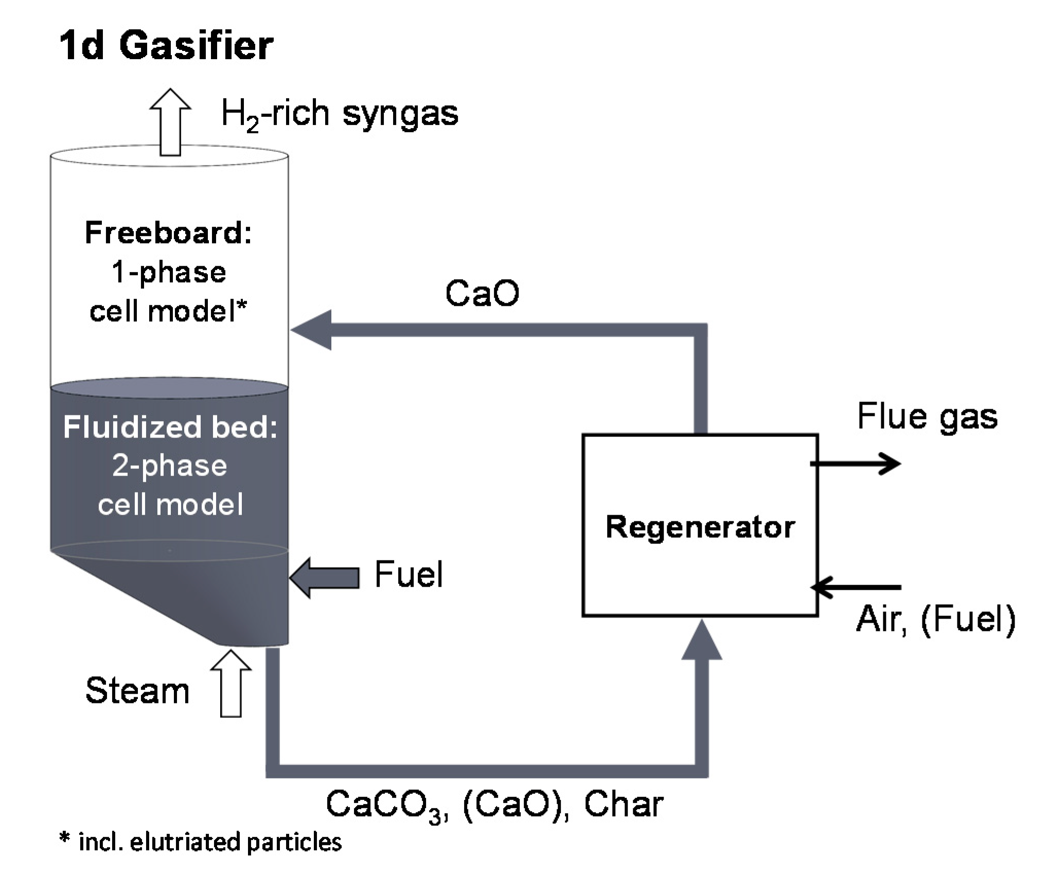
2.2. Development of a Dual Fluidized Bed Gasifier Model
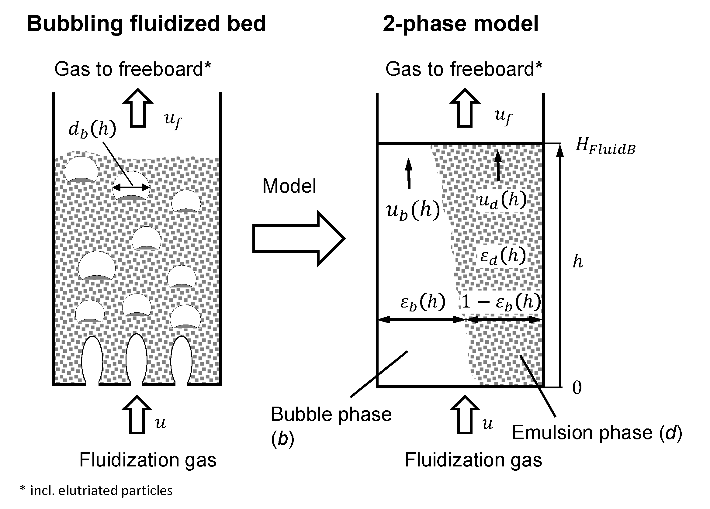
In Figure 2, the SEG modeling concept considered in this work is illustrated. The proposed model is based on details of the 200 kW dual fluidized bed (DFB) facility at the IFK. It consists of a bubbling fluidized bed (BFB) gasification reactor and a circulating fluidized bed (CFB) regenerator reactor. The gasifier model was discretized along the reactor length, in order to calculate all relevant transport values and for model validation purposes, to compare with the underlying experimental data. The regenerator is modeled in a simplified way, considering mass and energy balances as well as combustion and calcination reactions, in order to enable the coupling with the gasifier through the circulating solid.

2.3. Hydrodynamics

For modeling purposes, the fluidized bed was split into two phases, a solid-free bubble phase (fraction: εb) and a solid-loaded dense phase (fraction: 1-εb), as shown in Figure 3.

2.3.1. Dense Phase

In the model, the dense phase is considered to be a perfused pack with porosity εd and gas velocity ud. The calculation of ud and εd is performed following the methods presented by Hilligardt [26]. The minimum fluidization gas velocity, umf, is determined using the Ergun equation (Equation (1)), which is formulated based on the definitions of the Archimedes and Reynolds numbers, as well as the Sauter diameter (Equations (2)–(4)). In the present work, a sphericity of ψ = 0.75 [27] and a porosity at minimum fluidization εmf = 0.45 [27] are assumed.
A r = 150 1 ε m f ψ 2 · ε m f 3 R e m f + 1.75 ψ · ε m f 3 R e m f 2
A r = g · d s v 3 ν g 2 ρ p ρ g ρ g
R e m f = d s v · u m f ν g
d s v =   φ · d p ¯
Analysis of the fluidized bed inventory showed a mean particle size, d p ¯ , of 350 µm [11]. According to Hilligardt [26], the real velocity in the dense phase is higher than the calculated minimum fluidization gas velocity, umf, and it can be estimated with the following empirical equation:
u d | h = 0 =   u m f +   1 4 ( u e m p t y | h = 0   u m f )
For the remaining reactor heights ud(h) is determined by the continuity equation.
The porosity εd is calculated, as proposed by Richardson and Zaki [28], as
ε d ( h ) = ε m f ( u d ( h ) u m f ) 1 n R z .
For the parameter nRz, Richardson and Zaki [28] provided the empirical equation:
n R z = { 4.65 if   R e s 0.2 4.4 · R e s 0.03 if   0.2 R e s 1 4.4 · R e s 0.1 if   1 R e s 500 2.4 if   R e s > 500
where Res is the Reynolds number from the rate of descent of a single particle. In this work, the parameter nRz is used to adjust the calculated bed height to the experimental values. With nRz = 5.5, the model could be fitted to the real bed height determined experimentally.

2.3.2. Bubble Phase

Werther [29] developed a model (Equation (8)) to determine the bubble diameter, db, depending on the height of the fluidized bed, taking into account the coalescence and separation of the bubbles:
d ( d b ) d h = ( 2 ε b 9 π ) 1 / 3 d b 3 · 280 u m f g · u b * ( h )
At the position h = 0, the initial bubble diameter is calculated using the correlation d b = 1.3 ( V ˙ s t e a m 2 / g ) 0.2 , according to Tepper [27] and Davidson [30]. The initial bubble diameter depends on the volume flow of steam, V ˙ s t e a m , through an orifice of a gas distributor. The ascent velocity, u b * , of a bubble can be determined by Equations (9)–(11) from Hilligardt [26] and Tepper [27]:
u b * = 4 g d b 3 C D , b
C D , b = 16 R e b + 2.64
R e b = d b · u b * ν d   with   ν d = 60 · d s v 3 / 2 · g 1 / 2 .
The parameter CD,b is the drag coefficient of a single bubble and νd is the viscosity of the suspension phase. However, the ascent velocity u b * does not equal the gas velocity in the bubble phase ub, as the bubbles are additionally perfused by gas streams coming from the suspension phase [26,27]. Following the method proposed by Hilligardt [26], the gas velocity ub can be determined using the following empirical correlation:
u b = u b * + 2.7 u d

2.3.3. Fluidized Bed Height

With a defined inventory of the fluidized bed, MFluidB, the height of the fluidized bed, HFluidB, can be calculated by integrating the solid mass along the axial co-ordinate h [27]:
M F l u i d B = 0 H F l u i d B ( 1 ε b ) ( 1 ε d ) ρ p A c d h

2.3.4. Elutriation Rate

When gas bubbles rise to the surface of the fluidized bed and break, solid particles are thrown into the freeboard and entrained by the upward gas volume flow [31]. While the major fraction of these particles fall back into the fluidized bed, small particles whose terminal velocity is lower than the gas velocity are elutriated from the freeboard [31].
In the 200 kW facility, a cyclone is installed at the exit of the freeboard to reduce the extraction of bed inventory by leading the particles back into the fluidized bed [11]. It is assumed that there is an additional CO2 capture effect in the freeboard: Due to lower freeboard temperatures, the position of the chemical equilibrium can be changed, which enables a further carbonation reaction. However, as bigger particles fall or are transferred back into the fluidized bed by the cyclone, it is assumed that only fine particles have a contribution to the additional carbonation reaction. According to [31], the elutriation rate of particles (in g/s) is described by
M ˙ e l u t = k e l u t x f i n e
Herein, k e l u t is the elutriation rate constant and the weight fraction of fine particles, xfine, present in the bed was identified by measurements at the 200 kW facility. With a secondary cyclone, a mean particle size d p ¯ of 25 µm of elutriated particles was found. Considering the particle size distribution of the raw limestone, it can be derived that fine particles do not originate from the make-up of the raw material. Thus, the source of these particles must be attrition or fragmentation effects. From experiments, a correlation was derived to calculate the weight fraction of the fine particles:
x f i n e = a 1 tanh ( ( u a 2 ) / a 3 ) + a 4 ,
with the parameters a1 = −0.12697, a2 = 0.71214, a3 = −0.01191, and a4 = 0.12807.

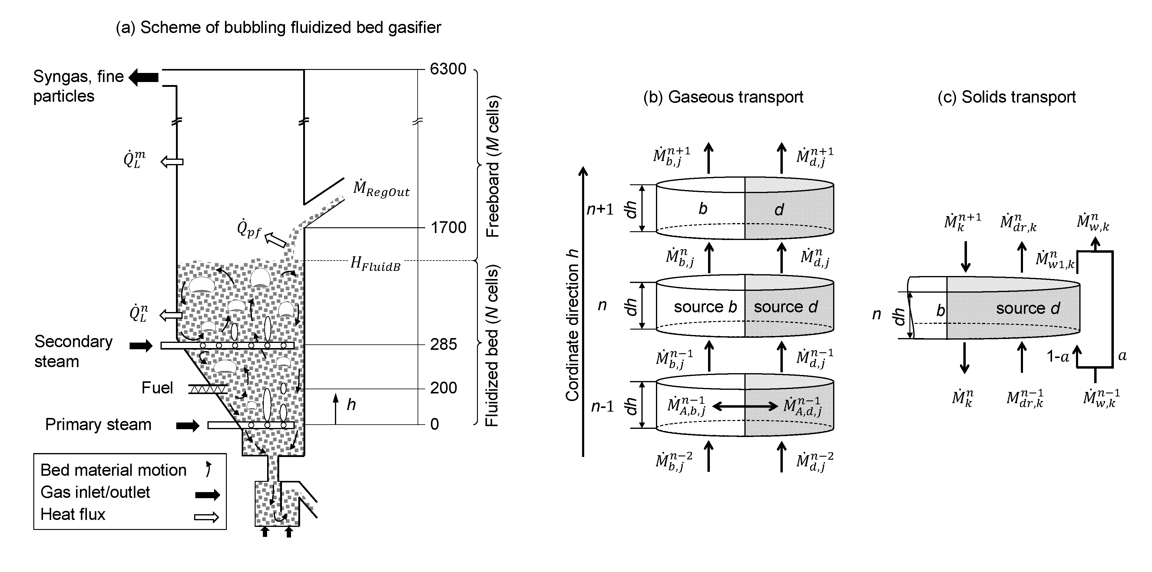
2.4. Gasifier Dimensions

In Figure 4a, a schematic diagram of the bubbling fluidized bed gasifier facility is shown, including the inlet/outlet gas and solid flows, as well as details of their axial position (in mm). These data were used to parametrize the simulation model. Here, M ˙ R e g O u t is the mass flow at the outlet of the regenerator to the gasifier. By tuning this mass flow rate, the desired gasification temperature can be achieved. The height of the fluidized bed, HFluidB, depends on the fluidization velocity and, hence, the distance between the inlet of M ˙ R e g O u t and HFluidB is variable.

2.5. Mass Balance

The gasifier is discretized along the reactor height. This includes the bubbling bed as well as the freeboard area. Figure 4b,c show how the calculation with axial discretization in cells proceeds through the fluidized bed for both gaseous and solid components. In each calculation cell of this 1d model, solid and gas components are considered to be fully mixed.

2.5.1. Fluidized Bed

According to the discretization shown in Figure 4b, the mass balance for each gaseous component in both dense phase (P = d) and bubble phase (P = b) is stated in Equation (16):
d M P , j n d t = 0 = M ˙ P , j n 1 M ˙ P , j n + M ˙ A , P , j n + M W j · I P ν i , j R P , i n + M ˙ i n , P , j n
where M ˙ P , j is the convective gas mass flow and M ˙ A , P , j is the exchange mass between bubble and suspension phases of component j in phase P; Ri is the reaction rate of reaction i and νi,j is the stoichiometric coefficient of component j in reaction i; IP describes the maximum number of reactions taking place in the phase and, with the term M ˙ i n , P , j , external inflows (e.g., from a secondary steam inlet) can be considered. Convective mass flows between adjacent calculation cells are defined by [27]
M ˙ d , j n = ρ d n u d n x d , j n ε d n A c n
M ˙ b , j n = ρ b n u b n x b , j n ( 1 ε d n ) A c n
The exchange between bubble and suspension phases inside the cell n is defined by [27]
M ˙ A , d , j n = K d b n A d b n ( ρ b n x b , j n ρ d n x d , j n )
M ˙ A , b , j n = K d b n A d b n ( ρ d n x d , j n ρ b n x b , j n )
According to Hilligardt [26], the mass transfer coefficient between the bubble and suspension phase is calculated as K d b n = 2.7 u d n 4 , and the mass exchange area over all bubbles in the cell n is A d b n = 6 ε b n · A c · d h / d b n . Additionally, overall mass balances for the suspension (P = d) and bubble (P = b) phases are developed in Equation (21), including the molar weight MWj of each component j:
d M P n d t = 0 = M ˙ P n 1 M ˙ P n + J M ˙ A , P , j n + J I P M W j ν i , j R i + M ˙ i n , P n .
Beside a balance for the gaseous components, a separate balance equation (Equation (22)) exists for the solids. According to Figure 4c, the amount of each solid component k in a calculation cell n is considered:
d M k n d t = 0 = M ˙ d r , k n 1 + ( 1 α ) M ˙ w , k n 1 + M ˙ k n + 1 M ˙ d r , k n M ˙ w 1 , k n M ˙ k n + M W j · I d ν i , k R d , k n + M ˙ i n , k n
The cell adjacent to the freeboard (n = N) additionally includes a sink term for elutriated fine particles M ˙ e l u t . It is important to split the mass balance into a description of gaseous and solid components as, in real plant operations, there exists a downward flow from the surface of the fluid bed (HFluidB) to the bottom (leaving the gasifier through the loop seal) and an upward flow due to the wake and drift of each rising gas bubble. Here, the term wake ( M ˙ w ) describes solids that fasten to the bubbles on their way upwards and drift ( M ˙ d r ) refers to solids that are loosely drawn upwards through the bubble movement. The solid transport by bubbles, together with the conical asymmetric cross section, see Figure 4a, in the lower part of the fluidized bed, leads to the strong exchange and motion of solids. To consider these effects, a model was developed in which the drift part of a rising bubble is fully mixed in each cell, whereas the proportion of wake that is mixed with or bypasses each cell can be chosen using the parameter α. The Term ( M W j · I d ν i , k R d , k n ) considers chemical reactions and with the term ( M ˙ i n , k n ) , inflows (e.g., from solid circulation) are included in the equation. The amount of solids which are transported with each bubble can be described by the empirical Equations (23) and (24) mentioned in [27]:
M ˙ w = A c ρ P ( 1 ε d ) ε b u b * · [ 0.59 0.046 ln ( A r ) ]
M ˙ d r = A c ρ P ( 1 ε d ) ε b · 0.38 u b * · [ 1.5 0.135 ln ( A r ) ]
In Figure 4c, the concept is illustrated to adapt the 1d model for gasification experiments with this highly three-dimensional behavior of the real system, through the adjustable parameter α.

2.5.2. Freeboard

The freeboard consists of a gas phase with a small amount of very fine particles with almost the same velocity. The gas component balance is
d M f , j m d t = 0 = M ˙ f , j m 1 M ˙ f , j m + M W j · I f ν i , j R f , i m
and the solid component balance is
d M k m d t = 0 = M ˙ k m 1 M ˙ k m + M W k · I k ν i , k R k , i m
Therefore, the overall mass balance expression is written as
d M m d t = 0 = M ˙ f m 1 + M ˙ k m 1 M ˙ f m M ˙ k m .
The linkage of the freeboard with the fluidized bed is carried out by applying Equation (28) for gases and Equation (29) for solids:
M ˙ f m = 0 = M ˙ d n = N + M ˙ b n = N
M ˙ k m = 0 = M ˙ e l u t

2.6. Energy Balances

2.6.1. Fluidized Bed

For each cell, a thermally fully developed mixture with a constant temperature is assumed. Therein, temperatures of solids and gases are equal; however, the temperature of the wake can differ, applying a vertical heat transfer between the cells.
Enthalpy fluxes for solids and gases are generally defined by mass flows: H ˙ = M ˙ · h . At the boundary of a cell, the enthalpy h of a mass flow of mixtures (e.g., gas inlet/outlet) is calculated as
h = J x j · h j ( T ) .
For solid mixtures, Equation (30) is written with index k. The temperature dependency of the enthalpy of a gas component j or a solid component k is calculated using polynomials from the software package FactSage®. In this approach, the enthalpies of the chemical reactions need not be considered additionally. The energy balance for a certain cell n is defined as
d H n d t = 0 = H ˙ d n 1 H ˙ d n + H ˙ b n 1 H ˙ b n + H ˙ k n 1 H ˙ k n + H ˙ d r n 1 H ˙ d r n + ( 1 α ) H ˙ w , k n H ˙ w 1 , k n + H ˙ i n n k F l u i d B π d r d h ( T n T c )
The last term of Equation (31) describes the heat loss through the reactor wall Q ˙ L n . It is calculated by using the temperature of the cooling jacket Tc = 40 °C and, by adapting to experimental pilot plant data, a heat transfer coefficient of kFluidB = 12.9 Wm−2K−1 was found.

2.6.2. Freeboard

The enthalpy balance for the freeboard section of the reactor can be expressed by
d H f m d t = 0 = H ˙ f m 1 H ˙ f m k f π d r d h ( T m T c ) + k p 6 d p ρ p M ˙ p m ( T p m T m ) · v p ,
where the term with the heat transfer coefficient, kf, describes the heat loss Q ˙ L , f m through the reactor wall in the freeboard section. A value of 3.4 Wm−2K−1 was selected by fitting the simulated temperature of the experimental temperature profile. According to the reactor design (see Figure 4a), hot solids from the regenerator ( M ˙ R e g O u t ) flow into the gasifier. However, the level of the inflow is located in the freeboard and above the surface of the fluidized bed (i.e., at position HFluidB). Hence, the particles pass the lower region of the freeboard before they dip in the fluidized bed. In this region, heat transfer Q ˙ p , f m between solid particles (p) and the gas phase (f) of the freeboard occurs. For this, a heat transfer coefficient, kp, with a value of 160.7 Wm−2K−1 was determined, which is well-aligned with values reported in the literature [32,33]. The temperature, T p n , of the bed material in the region between the inlet and fluidized bed is calculated by solving the energy balance:
d H p n d t = 0 = M ˙ R e g O u t c p , p n + 1 T p n + 1 M ˙ p c p , p n T p n k p f 6 d p ρ p M ˙ p ( T p n T n ) · v p
In this case, T p m = m i n = T R e g O u t and vp describes the velocity of a falling particle.

2.7. Chemical Reactions

Table 1 lists all the chemical reactions considered in the model, including equations to calculate the reaction rates. The pyrolysis step (reaction 1) is modelled with a one-step reaction kinetic considering the products: Ash, char, H2O, gases (CO2, CO, CH4, and H2), non-condensable hydrocarbons (simplified as C2H4), and tars (simplified as Naphthalene: C10H8). For the mass fractions ωj, experimental data from Fagbemi et al. [34] were used and interpolated to consider a temperature-dependent pyrolysis product composition. The values for the amounts of tar, however, originate from experiments with the 200 kW DFB system [19] and, hence, secondary pyrolysis reaction modelling was not required. With this assumption, catalytic effects of CaO on tar conversion are indirectly considered by measured concentrations. Residual char was handled as a mixture of C, H, and O and, according to the char analysis from Fagbemi et al. [34], the composition was also interpolated for different gasification temperatures. It is worth noting that the used elemental analysis of wood pellets (C: 48.99 wt.-%waf, H: 6.97 wt.-%waf, O: 44.04 wt.-%waf) differed from the analysis of biomass in Fagbemi et al. [34]. Thus, yields from pyrolysis ωj needed to be adapted, in order to satisfy the elemental balance. Therefore, a linear equation system for the elements C, H, and O had to be solved. While coefficients from C10H8, CH4, C2H4, H2O, and char were fixed, the coefficients of CO, CO2, and H2 were fitted to close the elemental balance of wood pellets.
Results for the mass fractions ωj are listed in Table A1. The reaction kinetics of ethene reformation (reaction 6) were adapted to fit the simulated H2 and CO concentrations to experimental values from the 200 kW DFB pilot plant. For the carbonation reaction, sorbent deactivation, which is dependent on the number of calcination–carbonation cycles, was taken into account through the parameter Xave. Details of the calculation of Xave are described in the subsequent section. For all gasification reactions, it is assumed that they occur only in the emulsion phase, due to the catalytic behavior of CaO and char, which enhance reaction rates compared to those in the gas phases [42].

2.8. Sorbent Deactivation

If limestone is subjected to several calcination–carbonation cycles, its CO2 sorption capacity is reduced, due to sintering phenomena on the particle surface [43]. For limestone, Grasa and Abanades [44] described the decay of the CO2 carrying capacity XN as
X N = 1 1 1 X r + k N + X r .
Equation (34) depends on the number of calcination–carbonation cycles N and uses the empirical constants k = 0.52 and Xr = 0.075. However, in a fluidized bed system, particles have different residence times, which leads to a distribution of the average CO2 carrying capacity. According to the references [45,46,47], an average carrying capacity Xave is calculated by a population balance:
X a v e = N = 1 F 0 F R ( 1 F 0 F R ) N 1 · X N
In the current study, Equation (35) was integrated into the model to calculate the average CO2 carrying capacity of the particle system with regard to the carbonation reaction (Table 1, Reaction 4). Therein, FR is the molar-based flow of M ˙ R e g O u t , describing the circulation flow of CaO from the regenerator into the gasifier. To compensate mass losses, mostly due to attrition, the reactor inventory was maintained by an input flow of raw limestone. In Equation (35), this input flow F0 was considered on a molar basis. As, in practice, the measured material flow of fresh limestone (by dosing units) contains particles which are small enough to be directly discharged, especially when feeding into the regenerator with fluidization velocities up to 5.5 m/s [11], it was assumed that F0 only represents the effective material flow that remains longer in the system. Fresh limestone and purge material are not considered in the mass and energy balance calculations, as their flow rates are very low compared to the circulating CaO mass flow. If this should be taken into account, detailed information is needed regarding the size of the particles and their degree of calcination when they are directly discharged from the regenerator due to their hydrodynamic properties.

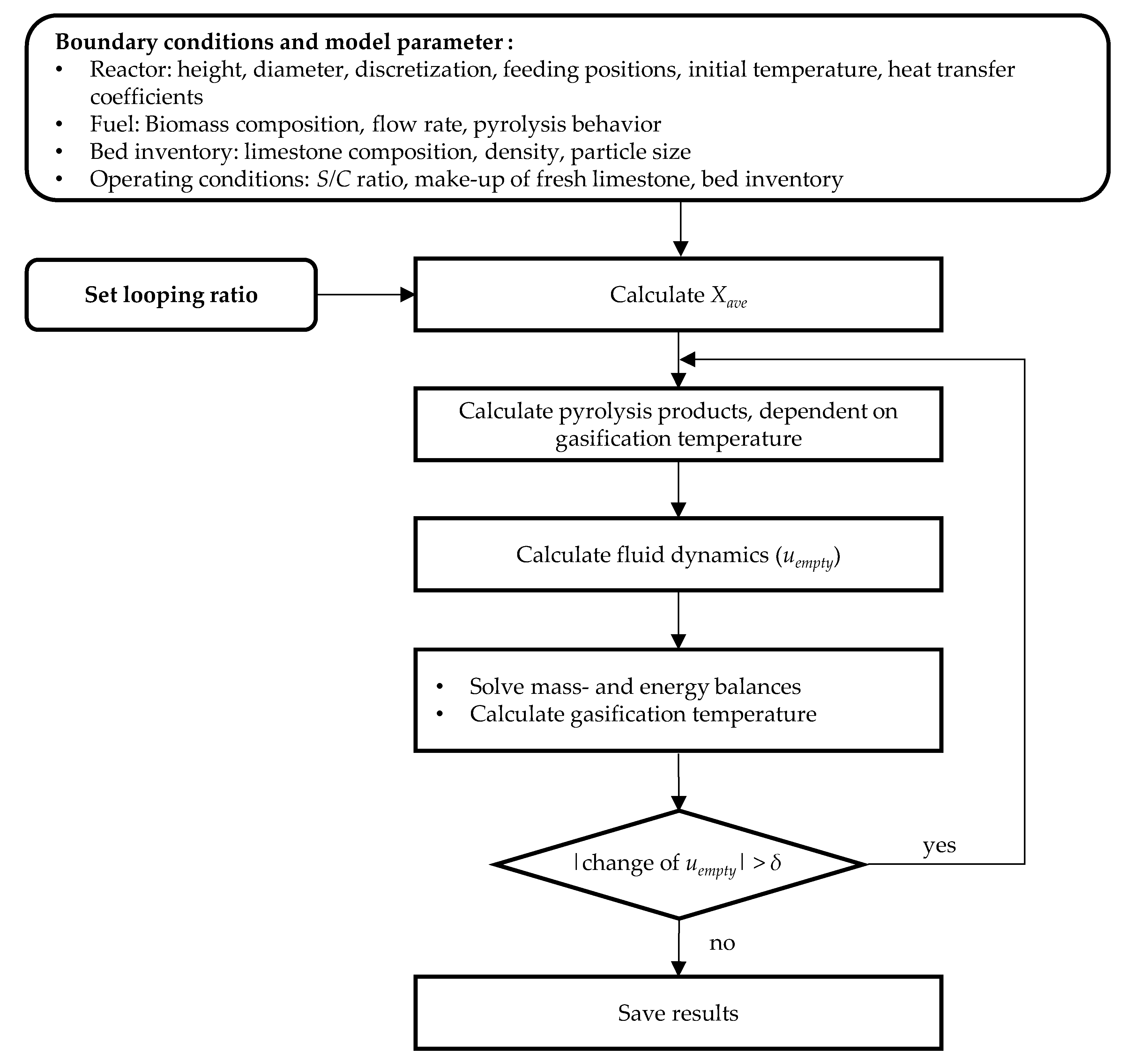
2.9. Simulation Algorithm

In the SEG system, internal solid circulation (mass flow from the Regenerator M ˙ R e g O u t ), the biomass feed stream, and the steam input are important parameters defining the gasification temperature. Therefore, in the simulation model, the molar calcium looping ratio ( F C a O / F C ) is used to set the gasification temperature. In this ratio, F C considers the molar flow of carbon contained in the biomass. The corresponding flow chart of the model is shown in Figure 5.
After setting boundary conditions and model parameters, the average CO2 carrying capacity is calculated using the make-up flow of fresh limestone and the looping ratio. Starting from an initial temperature, first the pyrolysis products and then the fluid dynamics of the gasifier are calculated. After solving the mass and energy balances, a new gasification temperature is calculated, and the pyrolysis step is updated for a certain looping ratio. This is iterated until the change of the empty reactor velocity, uempty, is smaller than a defined value δ; then, the results of the operation point are saved in a file.

3. Results and Discussion

In Section 3.1, the model parameters (e.g., heat transfer coefficients) are verified against experimental temperature data measured in the 200 kW fluidized bed gasifier [11]. Section 3.2 contains a model validation with measured gas compositions (H2, CO, CO2, CH4, C2H4), the lower heating value (LHV) of the syngas, and the M module from the 200 kW fluidized bed gasifier [11,19] in a temperature range of 600–850 °C. According to [48,49], the accuracy of the parameter verification and model validation was quantified by the sum squared deviation method:
MeanError :   E ¯ = n = 1 N ( φ e x p φ m o d e l φ e x p ) 2 N
For parameter verification, a low mean error of the temperature distribution along the reactor height of 10.6% was found. The model validation was carried out with a limestone make-up flow rate (MU) of 6.6 kg/h, according to experiments [11]. To characterize the effect of limestone make-up flow rate, a parametric study with 0.2 kg/h, 6.6 kg/h, and 15 kg/h is also included in the result diagrams. Mean errors to quantify the model prediction accuracy are listed in Table A2.

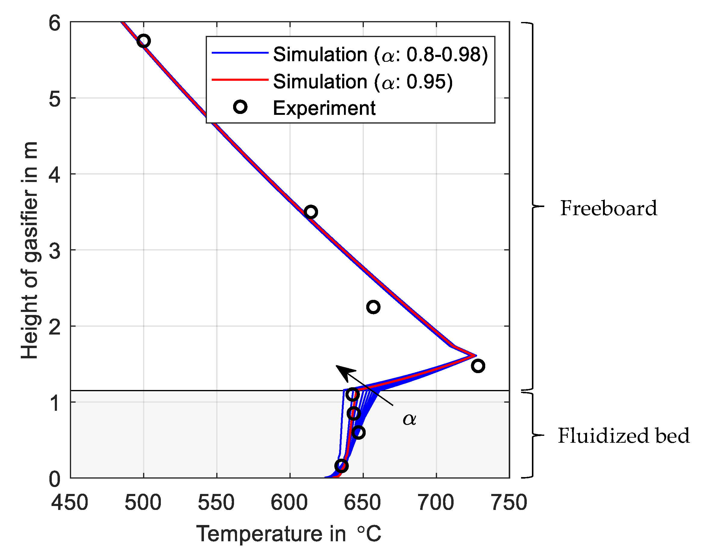
3.1. Verification of Model Parameter

In Figure 6, simulated temperature profiles from variations of the parameter α are compared with temperatures measured on different positions in the fluidized bed and the freeboard (available in [11]).
The profile of the measured temperatures (circles in Figure 6) over the height of the gasifier can be explained as follows: due to a good mixing of solids in the fluidized bed (0 m to 1.15 m) the temperatures were close to 640 °C, followed by an inflection, which was caused by the inlet of hot solids at 1.7 m (available thermocouple was at 1.5 m). In the freeboard above the solid inlet, a decrease of the gas temperature was observed due to heat losses through the reactor wall. A variation of the model parameter α in the range of 0.8–0.98 was carried out to adjust the fluidized bed temperature by changing the proportion of wake mixed within each discretization cell. From Figure 6, it can be seen that, with a value of α = 0.95 (red line), a temperature profile could be achieved, which corresponds to the measured temperature values. An almost vertical profile confirmed a homogeneous particle mixing in the fluidized bed. In the model, a heat transfer coefficient of kFluidB = 12.9 Wm−2K−1 was considered for the fluidized bed area. For the particle–gas heat transfer, a heat transfer coefficient value kp = 160.7 Wm−2K−1 and for the freeboard kf = 3.4 Wm−2K−1 were determined to describe the given temperature profile.

3.2. Validation with Experimental Data

After setting the model parameters, we carried out a verification based on temperature along the gasifier height, the syngas composition, LHV, reactions rates, and the M module, in order to compare the simulation results with experimental data over a temperature range from 600 °C to 850 °C.

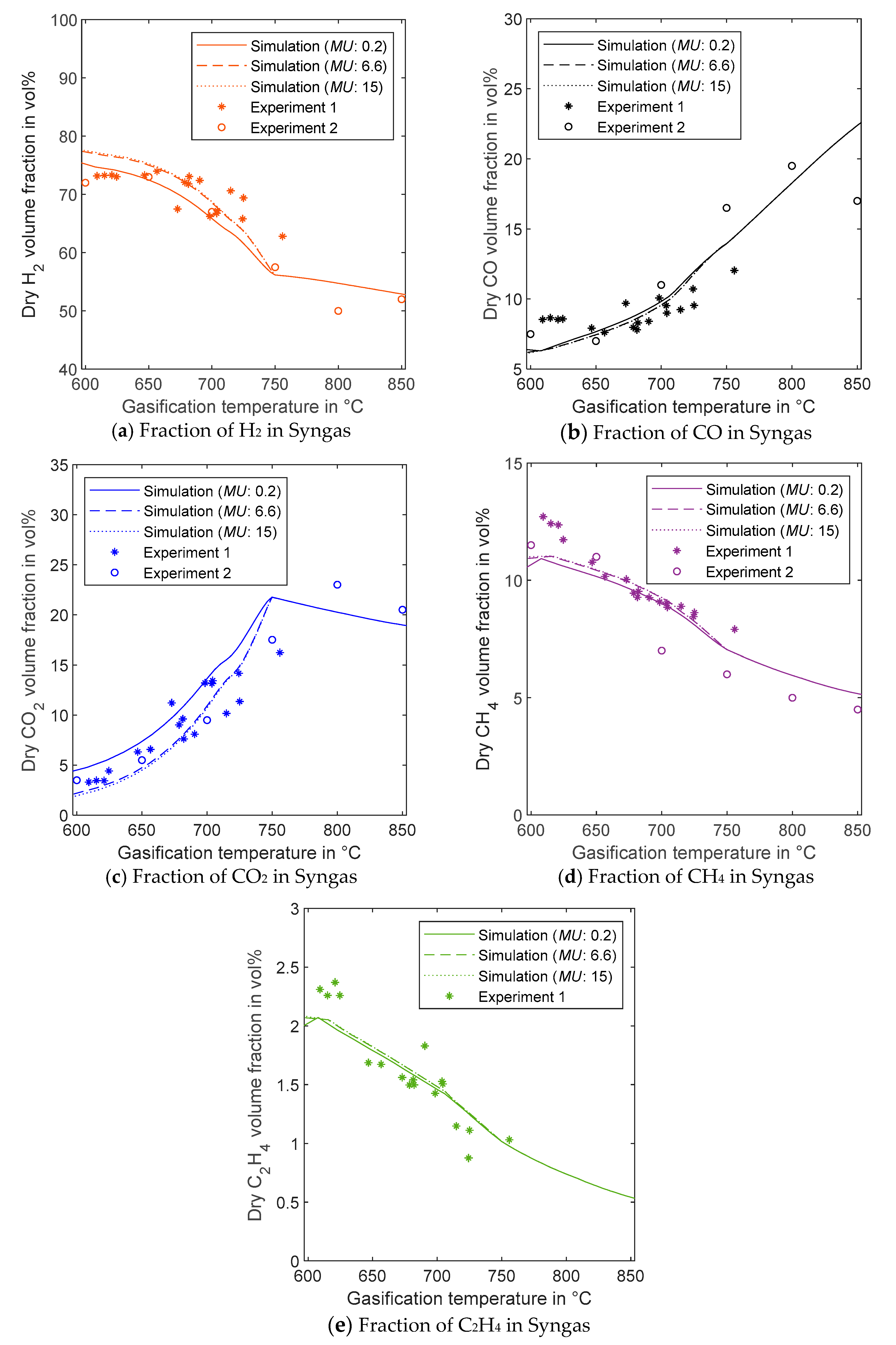
3.2.1. Effect of Gasification Temperature on Fractions of Syngas Components

In Figure 7a–e, the simulated volume fractions of synthesis gas components (H2, CO, CO2, and CH4) and non-condensable hydrocarbons (in the form of C2H4) are plotted over a gasification temperature between 600–850 °C. For each synthesis gas component, the curves of three different make-up flows (0.2 kg/h, 6.6 kg/h, and 15 kg/h) are shown to demonstrate its influence on the gas volume fraction. Additionally, experimental results derived from both 200 kW (Experiment 1) and 20 kW (Experiment 2) DFB systems are included to evaluate the simulated volume fractions.
For sorption enhanced gasification, one important characteristic is the strong dependency of the gas composition on the gasification temperature, which is affected by CO2 capture through the carbonation reaction [19,22]. Beside gasification reactions, the pyrolysis step also has an important impact on the initial gas composition in the fluidized bed [34]. The results from a 20 kW system were additionally included in the present work, as it enables operation temperatures up to 850 °C due to its electrical heating system. For low gasification temperatures, there is a larger distance between the actual CO2 concentration and the equilibrium curve for the carbonation/calcination regime [37,38]. This leads to a strong capture of CO2 and, hence, low CO2 concentrations in the syngas. With higher temperatures, the CO2 capture rate decreases and, consequently, the CO2 concentration in the syngas rises. Furthermore, this influences the water–gas shift reaction, resulting in decreased H2 concentrations and increased CO concentrations. When the CO2 concentration reaches the equilibrium concentration at around 750 °C, an inflection in the concentrations of CO2 and H2 can be observed. This demonstrates the strong coupling of the carbonation reaction with the water–gas shift reaction. Particularly for low gasification temperatures, there is also a distinctive influence of the make-up flow. Presumably, the reason for this effect is a reduced circulation mass flow of fresh CaO from the regenerator with a simultaneously higher CO2 capture rate due to lower temperatures. For instance, at a gasification temperature of 600 °C, the delivered circulation mass flow is around ten times lower, compared to that when operating at 850 °C. This can lead to a higher content of carbonated particles if the bed inventory is hardly exchanged. In this operating range, an increase of the limestone make-up rate can increase the activity in the bed and, thus, the CO2 capture rate.

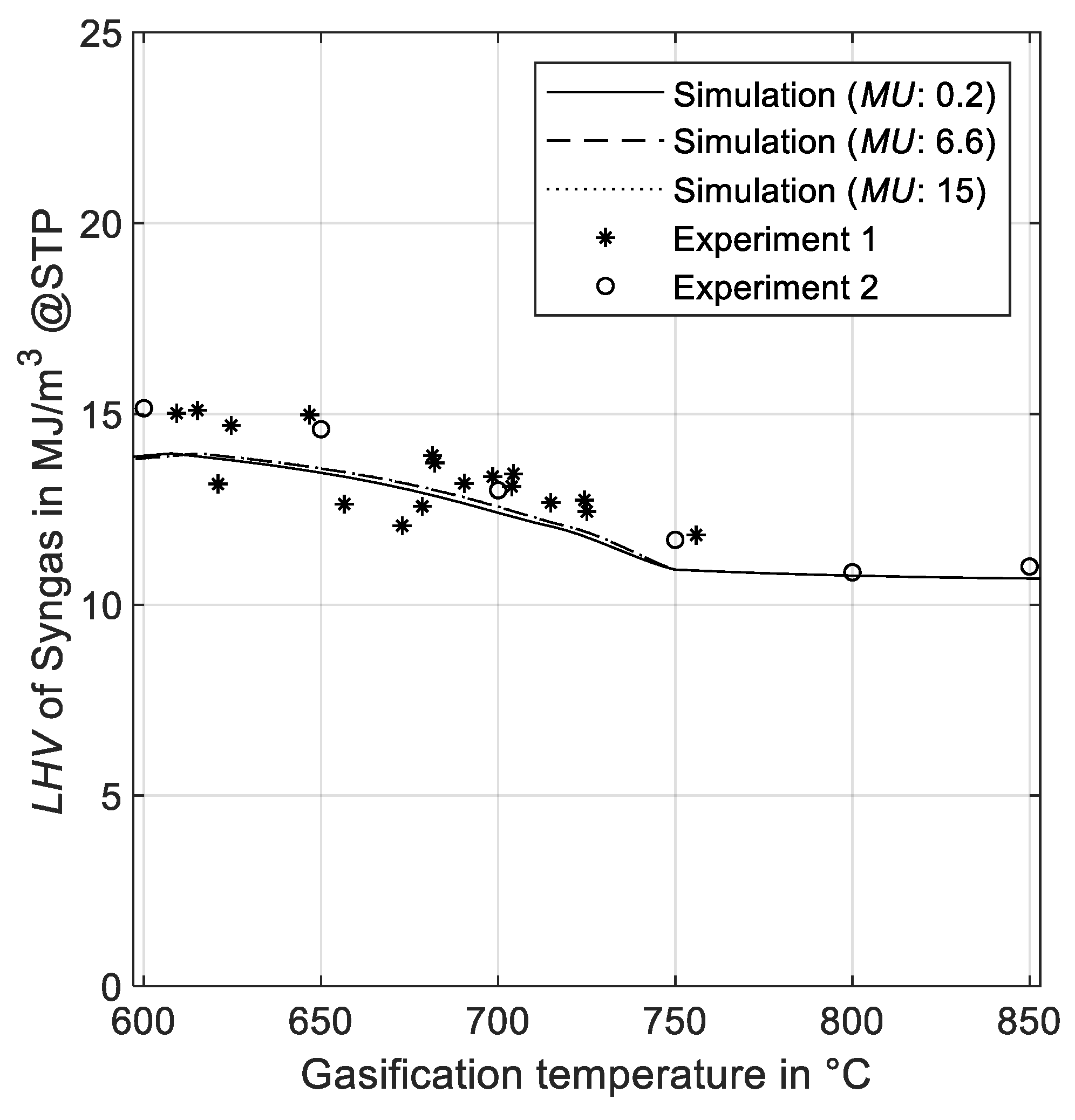
3.2.2. Effect of Gasification Temperature on LHV

As seen in Section 3.2.1, the gas composition is strongly affected by gasification temperature, due to the temperature dependence of (i) products released from pyrolysis, (ii) Arrhenius approaches to describe the gasification reactions, and (iii) carbonation/calcination equilibrium. Based on the lower heating values (LHV) of pure syngas components, the LHV of the gas mixture was calculated and compared with experimental data. In Figure 8, simulation results are shown over a temperature range of 600–850 °C and for different make-up flow rates.
The results show a good correlation with the experimental data and only a slight variation for different make-up flow rates is noticed. Furthermore, the effect of CO2 capture and its limitation at around 750 °C, recognizable as an inflection, can be described with this model. For higher temperatures, the LHV remains the same at a value of 10.9 MJ/m3 @STP. The highest values of LHV—around 14.5 MJ/m3 @ STP—can be reached at temperatures lower than 650 °C.

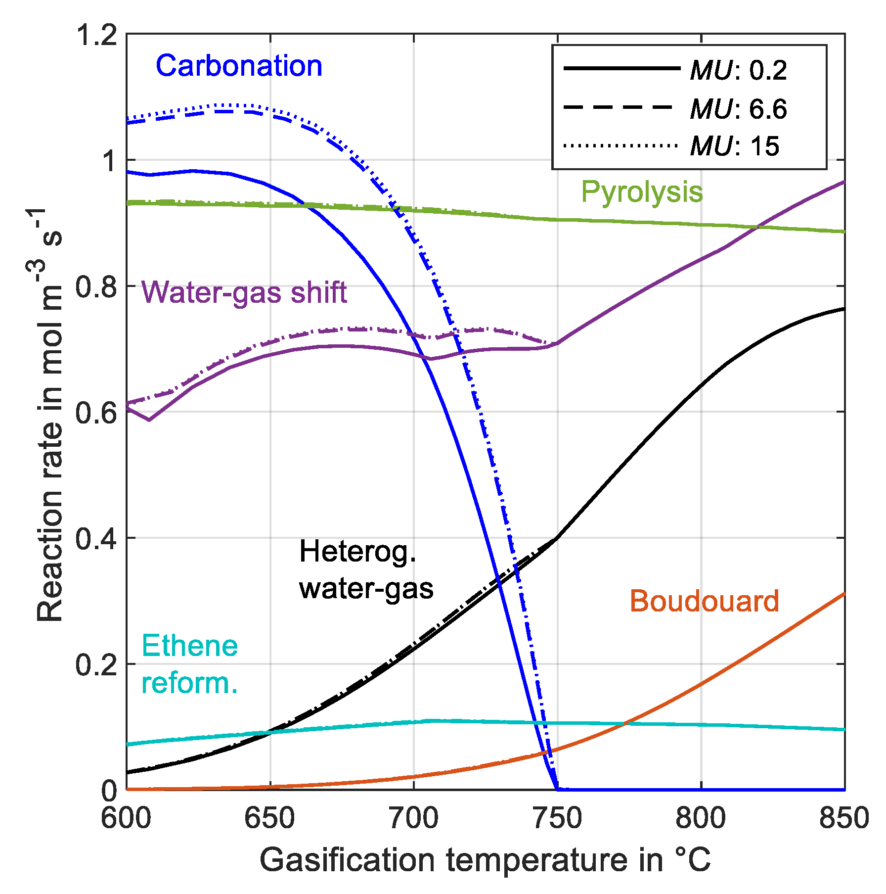
3.2.3. Effect of Make-Up Flow on Reaction Rate

In Figure 9, reaction rates (in mol m−3 s−1) are shown over a temperature range from 600 °C to 850 °C. Additionally, a variation of the make-up flows (0.2 kg/h, 6.6 kg/h, and 15 kg/h) was included to investigate the influence of sorbent deactivation on all considered reaction rates for the gasification process.
As the gasification temperature varies with changes of the circulation mass flow, the sorbent residence time differs and, according to Equation (35), the sorbent activity is also affected. It can be seen that deactivation mostly influenced the carbonation (reaction 4) and water–gas shift (reaction 5) reactions. For instance, for a constant temperature and a constant circulation mass flow, the carbonation reaction rate is higher with larger amounts of fresh limestone.
Considering the influence of the gasification temperature on the reaction rates, it can be seen that the reaction rates of the water–gas shift (reaction 5), the heterogeneous water–gas (reaction 2), and the Boudouard (reaction 3) reactions increased with higher temperatures. In contrast, for the pyrolysis (reaction 1) reaction, a minor decrease can be observed, even though an increase should be expected with higher temperatures. The reason for this behavior can be explained as follows: The amount of biomass in the fluidized bed system is limited by a constant fuel input flow. When the gasification temperature is increased, the reaction rate increases but, at the same time, a higher solid circulation is required for the higher temperature. Hence, more unreacted biomass is extracted from the gasifier through the loop seal, thus reducing the gas yield. Kinetic parameters of the Arrhenius approach influence the gradient of reactions for increasing temperatures. Comparing the Arrhenius parameters listed in Table 1, it can be seen that the influence of temperature on the heterogeneous water–gas shift reaction (reaction 2) was higher than that of the pyrolysis reaction (reaction 1).

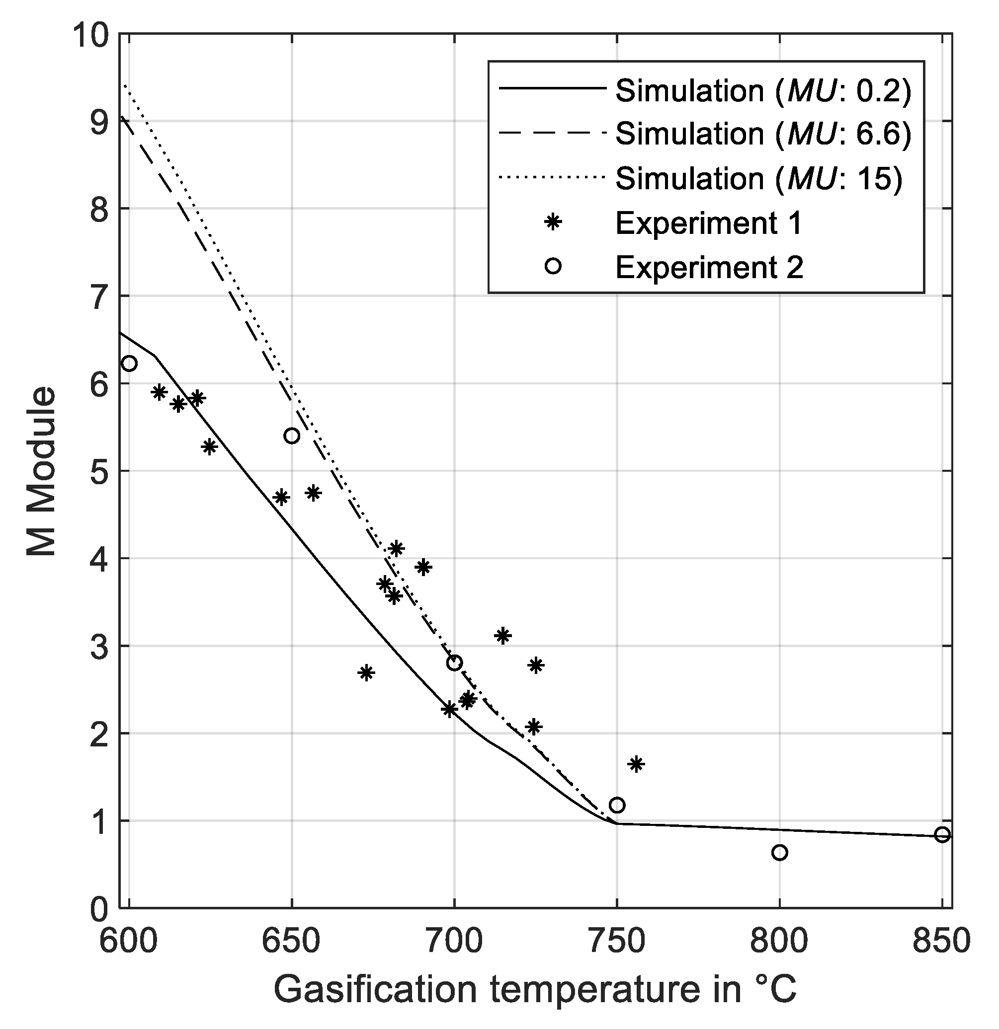
3.2.4. Effect of Gasification Temperature and Make-Up of Fresh Limestone on M Module

The M module from Equation (37) relates the gas concentrations of hydrogen, carbon dioxide, and carbon monoxide and has been considered as an important parameter which dictates the application of syngas [50]. For validity of an ideal gas, it can be written with volume fractions.
M = y H 2 y C O 2 y C O 2 + y C O
For instance, a M module of two is required for full stoichiometric conversion into dimethyl ether [50] and, for methane synthesis, a value of three can be derived from methanation reactions. Higher values are mostly interesting for hydrogen production. Figure 10 shows the influence of the gasification temperature on the M module. Additionally, three different simulation results, with a limestone make-up of 0.2 kg/h, 6.6 kg/h, and 15 kg/h, are compared with experimental data. It can be seen that a higher make-up flow enables higher M modules under the same gasification temperature.
For a low gasification temperature, the experimental data can be reached with a make-up flow of 0.2 kg/h. At a gasification temperature above 650 °C, the simulation model with a make-up flow of 6.6 kg/h precisely describes the experimental data. This parametric study reveals that the make-up flow is an important factor when optimizing the gasification process for a certain application. When considered from an economic point of view, operation strategies with low make-up rates are preferable.

4. Sensitivity Analysis of Fuel Feeding Rate

For a realistic and flexible operation of the biomass gasification process, it is important that the process allows for safe operations under a wide load range. In this section, the effects of different fuel feeding rates on the bed height, the fluidization level (gas velocity ratio: superficial gas velocity u based on minimum fluidization velocity umf), and the power of the syngas, depending on the gasification temperature, are investigated.

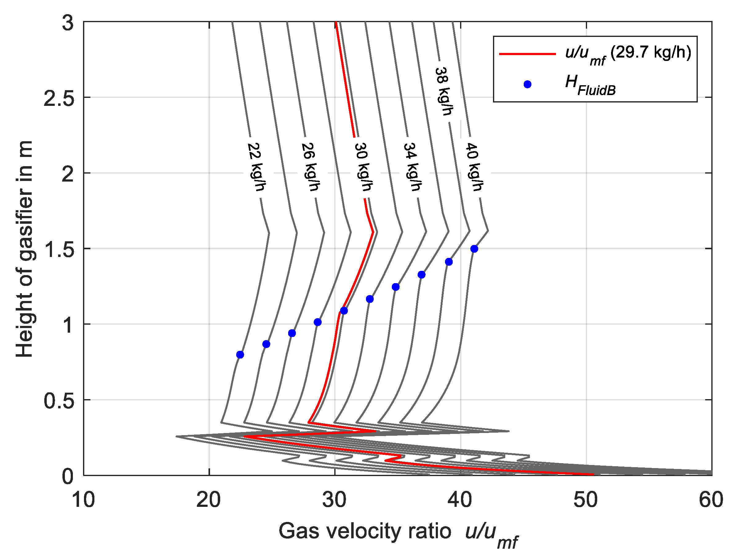
4.1. Effect of Biomass Feeding Rate on Bed Height and Gas Velocity Ratio

The model was also used to study the influence of different biomass feeding rates on the hydrodynamics in the fluidized bed. In Figure 11, the gas velocity ratio (superficial gas velocity/minimum fluidization gas velocity) is shown over a height of 3 m of the gasifier focusing on the fluidized bed and lower part of the freeboard. In this figure, the biomass feeding rate is considered as curve parameter in the range of 22–40 kg/h, whereby the operating point considered in Section 3.1 (feeding rate: 29.7 kg/h) was additionally drawn as a red line. Since the fluidized bed expands with larger fluidization volume flows, the diagram also shows the height of the fluidized bed for the different biomass feeding rates as blue dots. This allows the gas velocity at the surface of the fluidized bed to be read directly from the diagram.
It can be seen that with a higher biomass feeding rate, the gas velocity ratio increased at any position in the reactor. The reason is that when biomass particles pyrolyze in a fluidized bed, the released gas contributes to the reactor fluidization. In addition, a constant S/C ratio of 2.2 was selected for the simulations, in order to maintain a stable syngas quality [51] and to ensure comparability with the experimental data [11]. This changes the amount of steam supplied and, hence, the gas velocity ratio. In Figure 11, the red line corresponds to the same case which was considered for model verification in Section 3.1, with the reactor temperature in the axial direction. At the zero position in y-axis, the primary steam inlet is located. Due to the smallest cross-section in this area (compare Figure 4a), the highest gas velocity ratios were found here. On higher levels of the gasifier, the diameter of the reactor increases, which leads to a decrease of the gas velocity ratio due to the continuity equation. However, increasing velocities can be observed resulting from the gas release due to biomass pyrolysis (h = 0.2 m) and the secondary steam inlet (h = 0.285 m). At h ≥ 0.35 m, the reactor has a cylindrical shape and from the constant cross section in combination with further biomass pyrolysis, the gas velocity ratio slightly increases. In the freeboard above the inlet of solids, the temperatures decrease due to heat losses, and hence, the gas velocity ratio decreases. This is indicated by an inflection in the gas velocity ratio curves at a height of 1.7 m. Looking at the fluidized bed height for operation with 22 kg/h and 40 kg/h biomass feeding rate, one can see that the height doubles. For the case with 40 kg/h, the bed height (blue dots) almost reaches the area of the inlet for the solid circulation at 1.7 m. In order to ensure stable operation with this reactor geometry, operating modes that lead to a further increase in bed height should be avoided.

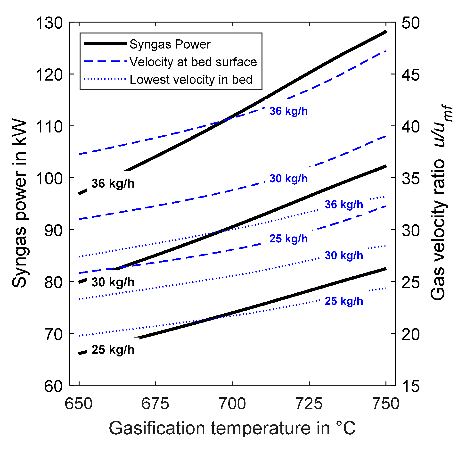
4.2. Performance Diagram for Gasifier Operation

Based on the results derived from this work, a performance diagram of the bubbling fluidized bed gasifier was created in Figure 12. This relates the selected gasification temperature (based on downstream requirements of the syngas composition) and fuel feeding rate to the power of the syngas. Additionally, the gas velocity ratio from the superficial gas velocity at the fluidized bed surface and the gas velocity ratio for the lowest velocity in the fluidized bed are depicted.
By combining the gasification chemistry (which lead to the syngas power) and the hydrodynamic information (represented as the gas velocity ratio), it is possible to identify a realistic operational range of the gasifier.
With a gasification temperature of 650 °C and 25 kg/h fuel input, the lowest gas velocity ratio of 20 could be identified. This means that, in any position of the fluidized bed, the superficial gas velocity was 20 times higher than the minimum fluidization velocity. Hence, good mixing of the bed inventory can be assured. At the bed surface, the superficial gas velocity was 26 times higher than the minimum gas velocity and only a little particle extraction can be expected. Increasing the fuel feeding rate to 36 kg/h at 650 °C, the syngas power increased and reached almost 100 kW. At this point, the velocity at the surface of the fluidized bed increased by a factor of 37 (related to umf) and by a factor of 27 (related to umf) for the lowest velocity in the bed. By increasing the gasification temperature and the gasifier feeding rate up to 750 °C and 36 kg/h, respectively, good mixing in the fluidized bed is guaranteed. However, due to the high velocity at the bed surface (a factor of 47 related to umf), a high particle extraction has to be accounted for. To avoid this negative effect, the fuel input or the gasification temperature can be modified. In that case, the syngas composition is not very important for downstream applications, an identical syngas power (around 100 kW) can be reached for a gasification temperature of 750 °C and 30 kg/h fuel input or for an operation with 650 °C and with a fuel input of 36 kg/h. However, the operational point at 650 °C reduced particle extraction from the gasifier due to the non-linear behavior of the gas velocity ratio curves.

5. Conclusions

The one-dimensional sorption enhanced gasification model developed in this study was verified with experimental data obtained from a 200 kW facility at IFK, University of Stuttgart. The results showed that the model is able to successfully predict the performance of the pilot plant at different operation conditions. With this model, the influence of important process parameters, such as gasification temperature, steam-to-carbon ratio, solid inventory, and fuel mass flow, can be simulated. On the basis of gas composition (H2, CO, CO2, CH4, and C2H4), LHV, and the M module, the model was validated over the whole SEG temperature range. As the activity of the limestone sorbent decreases after several carbonation/calcination cycles, an additional model was integrated, which adapts the carbonation reaction kinetics depending on the circulation rate and molar flow of fresh limestone. With this possibility, three different fresh limestone make-up flow rates (0.2 kg/h, 6.6 kg/h, and 15 kg/h) were simulated. A parametric study revealed a larger dependence on the limestone make-up, especially for gasification temperatures below 650 °C. This effect probably has to do with the lower circulation rate between gasifier and regenerator and the reduced transfer of fresh CaO into the gasifier with different CO2 capture activities. Increasing the make-up flow rate also increases the bed activity for the same quantity of mass transferred into the gasifier. At higher temperatures, it can be assumed that this effect is reduced by limitations of the carbonation reaction equilibrium. Considering the reaction rates in the temperature range between 600 and 750 °C, a strong dependency of the limestone make-up on the carbonation reaction can be identified. Furthermore, the water–gas shift reaction is influenced due to the CO2 capture. For the other reactions considered, only a minor influence from the limestone make-up was observed.
Variation of the fuel feeding rate (22 kg/h to 40 kg/h) with a constant S/C ratio (2.2 mol/mol) revealed an increase of the bed height by a factor of 2. From the gas velocity ratio (u/umf) along the reactor height, different fluidization states can be recognized. While a low fuel input led to low mixing in certain areas of the fluidized bed (u was only higher than umf by a factor of 20), high fuel input increased mixing in the whole fluidized bed. However, the entrainment of particles was also higher. Based on these evaluations, the syngas power and the gas velocities of the bubbling fluidized gasifier were described in a performance diagram which is dependent on the gasification temperature and the fuel input. Therefore, the developed model can be used as a fast and reliable engineering tool for reactor design or scale-up purposes.

Author Contributions

M.B. is responsible for conceptualization, simulation studies, validation, and original draft preparation. M.B. and M.S. designed the methodology of the software. Writing—review and editing, A.M.P.; supervision, G.S. All authors have read and agreed to the published version of the manuscript.

Funding

This research was funded by Ministry of the Environment Baden-Württemberg, Germany, grant number BWE13008.

Acknowledgments

The authors gratefully acknowledge financial supports from the project BioenergieFlex (BWE13008) funded by the Ministry of the Environment Baden-Württemberg, Germany.

Conflicts of Interest

The authors declare no conflict of interest.

Nomenclature

Aarea (m2)
ArArchimedes number (-)
CD,bdrag coefficient of a bubble (-)
c j m a s s concentration of component j (kg/m3)
c j concentration of component j (mol/m3)
c p specific heat capacity (J kg−1K−1)
d s v Sauter diameter (m)
d diameter (m)
E ¯ mean Error (-)
F 0 flow of fresh CaCO3 (mol/s)
F R flow of circulating CaO (mol/s)
F C flow of elemental carbon in fuel flow (mol/s)
gacceleration of gravity (m/s2)
Hheight (m)
H ˙ enthalpy flow (J/s)
henthalpy (J/kg)
hreactor co-ordinate (m)
Imaximum number of chemical reactions (-)
Jmaximum number of components (-)
K d b mass transfer coefficient (m/s)
kheat transfer coefficient (W m−2K−1)
kempirical constant for sorbent deactivation (-)
kelutelutriation rate constant (here in g/s)
LHVlower heating value (MJ/m3)
Mmass (kg)
Msyngas module (mol/mol)
Mmaximum number of cells in freeboard (-)
M ˙ mass flow (kg/h, g/s)
MUmake-up flow of fresh limestone (kg/h)
MWmolar weight (kg/kmol)
mdiscretization cell in freeboard (-)
Nnumber of calcination-carbonation cycles (-)
Nmaximum number of cells in fluidized bed (-)
ndiscretization cell in fluidized bed (-)
n R Z parameter for descent rate of single particle in suspension phase
p j partial pressure of component j (-)
Q ˙ heat flux (J/s)
ReReynolds number (-)
Rreaction rate (mol/s, kg/s)
rreaction rate (mol s−1m−3, kg s−1m−3)
S/Csteam-to-carbon ratio (mol H2O/mol carbon)
TTemperature (K)
ttime (s)
usuperficial gas velocity (m/s)
u m f minimum fluidization gas velocity (m/s)
u b * ascent velocity of bubble (m/s)
V ˙ volume flow (m3/h)
v p particle falling velocity (m/s)
WHSVweight hourly space velocity (1/h)
X a v e average CO2 carrying capacity (mol CaCO3/mol Ca)
X N CO2 carrying capacity after N cycles (mol CaCO3/mol Ca)
Xrempirical constant for sorbent deactivation (-)
xmass fraction (-)
yvolume fraction (-)
αfraction of mass exchange in calculation cell (-)
δprecision of numerical calculation
εporosity (-)
νkinematic viscosity (m2/s)
νstoichiometric coefficient (-)
ρdensity (kg/m3)
ψsphericity of particles (-)
ωjmass fraction of pyrolysis product j (-)
BMbiomass
bbubble phase
ccross section in reactor
demulsion phase
drdrift
eqequilibrium
elutelutriation
emptycondition in empty reactor tube
ffreeboard
ggas
iindex of chemical reaction
ininlet flow via boundary condition
jindex of gas component
kindex of solid component
mfcondition at minimum fluidization
pparticle
rreactor
wwake
wfwater-free

Appendix A

Table A1. Mass fractions (ωj) of products from biomass pyrolysis in the temperature range of 600–800 °C; values from Fagbemi et al. [34] adapted for pyrolysis of wood pellets.
Component600 °C650 °C700 °C750 °C800 °C850 °C
Ash0.00320.00320.00320.00320.00320.0032
Char0.24730.24830.24510.24350.24120.2324
H2O0.16540.15080.13300.13120.12910.1243
CO20.24750.24330.28070.25140.22930.1890
CO0.17060.20170.18510.22460.25560.3145
CH40.05230.05810.06320.06310.06290.0619
H20.02510.02690.02840.02960.03080.0326
C2H40.03990.04570.05090.04820.04530.0407
C10H80.04880.02210.01040.00520.00270.0014
Table A2. Comparison of experimental and simulated data with method of mean error.
Simulated ValuesMean Error in %,
MU: 0.2 kg/h
Mean Error in %,
MU: 6.6 kg/h
Mean Error in %,
MU: 15 kg/h
H2—Composition vs. Temperature (°C)5.54.95.0
CO—Composition vs. Temperature (°C)15.715.315.3
CO2—Composition vs. Temperature (°C)33.922.825.1
CH4—Composition vs. Temperature (°C)7.26.66.5
C2H4—Composition vs. Temperature (°C)14.114.314.2
LHV vs. Temperature (°C)6.75.95.9
M module vs. Temperature (°C)23.429.932.2
Partially higher mean errors can also be caused by large fluctuations in the measured values, as no filtering was performed.

References

  1. Statistics, I.E.A. CO2 Emissions from Fuel Combustion: Highlights; International Energy Agency: Paris, France, 2017. [Google Scholar]
  2. Olivier, J.G.J.; Schure, K.M.; Peters, J.A.H.W. Trends in Global CO2 and Total Greenhouse Gas Emissions; PBL Netherlands Environmental Assessment Agency: The Hague, The Netherlands, 2017. [Google Scholar]
  3. Göransson, K.; Söderlind, U.; He, J.; Zhang, W. Review of syngas production via biomass DFBGs. Renew. Sustain. Energy Rev. 2011, 15, 482–492. [Google Scholar] [CrossRef]
  4. Rauch, R.; Hofbauer, H. Wirbelschicht-Wasserdampf-Vergasung in der Anlage Güssing (A); Betriebserfahrungen aus zwei Jahren Demonstrationsbetrieb. In Proceedings of the 9th International Symposium “Energetische Nutzung nachwachsender Rohstoffe”, Freiberg, Germany, 4–5 September 2003; FAU: Nuremberg, Germany, 2003. [Google Scholar]
  5. Thunman, H.; Larsson, A.; Hedenskog, M. Commissioning of the GoBiGas 20 MW Biomethane Plant. Proceedings of Tcbiomass 2015, Chicago, IL, USA, 2–5 November 2015; GTI: Des Plaines, IL, USA, 2015. [Google Scholar]
  6. Fiaschi, D.; Michelini, M. A two-phase one-dimensional biomass gasification kinetics model. Biomass Bioenergy 2001, 21, 121–132. [Google Scholar] [CrossRef]
  7. Lü, P.; Kong, X.; Wu, C.; Yuan, Z.; Ma, L.; Chang, J. Modeling and simulation of biomass air-steam gasification in a fluidized bed. Front. Chem. Eng. China 2008, 2, 209–213. [Google Scholar] [CrossRef]
  8. Puig-Arnavat, M.; Bruno, J.C.; Coronas, A. Review and analysis of biomass gasification models. Renew. Sustain. Energy Rev. 2010, 14, 2841–2851. [Google Scholar] [CrossRef]
  9. Gordillo, E.D.; Belghit, A. A two phase model of high temperature steam-only gasification of biomass char in bubbling fluidized bed reactors using nuclear heat. Int. J. Hydrog. Energy 2011, 36, 374–381. [Google Scholar] [CrossRef]
  10. Agu, C.E.; Pfeifer, C.; Eikeland, M.; Tokheim, L.-A.; Moldestad, B.M.E. Detailed one-dimensional model for steam-biomass gasification in a bubbling fluidized bed. Energy Fuels 2019, 33, 7385–7397. [Google Scholar] [CrossRef]
  11. Hawthorne, C.; Poboss, N.; Dieter, H.; Gredinger, A.; Zieba, M.; Scheffknecht, G. Operation and results of a 200-kWth dual fluidized bed pilot plant gasifier with adsorption-enhanced reforming. Biomass Convers. Biorefinery 2012, 2, 217–227. [Google Scholar] [CrossRef]
  12. Schweitzer, D.; Albrecht, F.G.; Schmid, M.; Beirow, M.; Spörl, R.; Dietrich, R.-U.; Seitz, A. Process simulation and techno-economic assessment of SER steam gasification for hydrogen production. Int. J. Hydrog. Energy 2018, 43, 569–579. [Google Scholar] [CrossRef]
  13. Rauch, R.; Hrbek, J.; Hofbauer, H. Biomass gasification for synthesis gas production and applications of the syngas. WIREs Energy Environ. 2014, 3, 343–362. [Google Scholar] [CrossRef]
  14. Inayat, A.; Ahmad, M.M.; Yusup, S.; Mutalib, M.I.A. Biomass Steam Gasification with In-Situ CO2 Capture for Enriched Hydrogen Gas. Production: A Reaction Kinetics Modelling Approach. Energies 2010, 3, 1472–1484. [Google Scholar] [CrossRef] [Green Version]
  15. Sreejith, C.C.; Muraleedharan, C.; Arun, P. Air–steam gasification of biomass in fluidized bed with CO2 absorption: A kinetic model for performance prediction. Fuel Process. Technol. 2015, 130, 197–207. [Google Scholar] [CrossRef]
  16. Hejazi, B.; Grace, J.R.; Bi, X.; Mahecha-Botero, A. Kinetic model of steam gasification of biomass in a bubbling fluidized bed reactor. Energy Fuels 2017, 31, 1702–1711. [Google Scholar] [CrossRef]
  17. Hejazi, B.; Grace, J.R.; Mahecha-Botero, A. Kinetic modeling of lime-enhanced biomass steam gasification in a dual fluidized bed reactor. Ind. Eng. Chem. Res. 2019, 58, 12953–12963. [Google Scholar] [CrossRef]
  18. Pitkäoja, A.; Ritvanen, J.; Hafner, S.; Hyppänen, T.; Scheffknecht, G. Simulation of a sorbent enhanced gasification pilot reactor and validation of reactor model. Energy Convers. Manag. 2020, 204, 112318. [Google Scholar] [CrossRef]
  19. Poboß, N. Experimentelle Untersuchung der Sorptionsunterstützten Reformierung. Ph.D. Thesis, Universität Stuttgart, Stuttgart, Germany, 18 May 2016. [Google Scholar]
  20. Wang, C.; Zhou, X.; Jia, L.; Tan, Y. Sintering of limestone in calcination/carbonation cycles. Ind. Eng. Chem. Res. 2014, 53, 16235–16244. [Google Scholar] [CrossRef]
  21. Pfeifer, C.; Puchner, B.; Hofbauer, H. Comparison of dual fluidized bed steam gasification of biomass with and without selective transport of CO2. Chem. Eng. Sci. 2009, 64, 5073–5083. [Google Scholar] [CrossRef]
  22. Koppatz, S.; Pfeifer, C.; Rauch, R.; Hofbauer, H.; Marquard-Moellenstedt, T.; Specht, M. H2 rich product gas by steam gasification of biomass with in situ CO2 absorption in a dual fluidized bed system of 8 MW fuel input. Fuel Process. Technol. 2009, 90, 914–921. [Google Scholar] [CrossRef]
  23. Schmid, M.; Beirow, M.; Schweitzer, D.; Waizmann, G.; Spörl, R.; Scheffknecht, G. Product gas composition for steam-oxygen fluidized bed gasification of dried sewage sludge, straw pellets and wood pellets and the influence of limestone as bed material. Biomass Bioenergy 2018, 117, 71–77. [Google Scholar] [CrossRef]
  24. Soukup, G.; Pfeifer, C.; Kreuzeder, A.; Hofbauer, H. In situ CO2 capture in a dual fluidized bed biomass steam gasifier—Bed material and fuel variation. Chem. Eng. Technol. 2009, 32, 348–354. [Google Scholar] [CrossRef]
  25. Schweitzer, D.; Beirow, M.; Gredinger, A.; Armbrust, N.; Waizmann, G.; Dieter, H.; Scheffknecht, G. Pilot-scale demonstration of Oxy-SER steam gasification: Production of syngas with pre-combustion CO2 capture. Energy Procedia 2016, 86, 56–68. [Google Scholar] [CrossRef] [Green Version]
  26. Hilligardt, K. Zur Strömungsmechanik von Grobkornwirbelschichten. Ph.D. Thesis, Technische Universität Hamburg, Hamburg, Germany, 1986. [Google Scholar]
  27. Tepper, H. Zur Vergasung von Rest-und Abfallholz in Wirbelschichtreaktoren für Dezentrale Energieversorgungsanlagen. Ph.D. Thesis, Universität Magdeburg, Magdeburg, Germany, 2005. [Google Scholar]
  28. Richardson, J.F.; Zaki, W.N. Sedimentation and fluidisation: Part I. Chem. Eng. Res. Des. 1997, 75, S82–S100. [Google Scholar] [CrossRef]
  29. Werther, J. Experimentelle Untersuchungen zur Hydrodynamik von Gas./Festoff-Wirbelschichten. Ph.D. Thesis, Technische Fakultät der Universität Erlangen-Nürnberg, Erlangen, Germany, 1972. [Google Scholar]
  30. Davidson, J.F. Bubble formation at an orifice in an inviscid liquid. Trans. Inst. Chem. Eng. 1960, 38, 335–342. [Google Scholar]
  31. Wen, C.Y.; Chen, L.H. Fluidized bed freeboard phenomena: Entrainment and elutriation. AIChE J. 1982, 28, 117–128. [Google Scholar] [CrossRef]
  32. Dietz, S. Wärmeübergang in Blasenbildenden Wirbelschichten. Ph.D. Thesis, Technische Fakultät der Universität Erlangen-Nürnberg, Erlangen, Germany, 1994. [Google Scholar]
  33. Zhang, D.; Koksal, M. Heat transfer in a pulsed bubbling fluidized bed. Powder Technol. 2006, 168, 21–31. [Google Scholar] [CrossRef]
  34. Fagbemi, L.; Khezami, L.; Capart, R. Pyrolysis products from different biomasses: Application to the thermal cracking of tar. Appl. Energy 2001, 69, 293–306. [Google Scholar] [CrossRef]
  35. Roberts, A.F.; Clough, G. Thermal decomposition of wood in an inert atmosphere. In Proceedings of the Ninth Symposium (International) on Combustion, New York, NY, USA, 27 August–1 September 1963. [Google Scholar]
  36. Hemati, M.; Laguerie, C. Determination of the kinetics of the wood sawdust steam gasification of charcoal in a thermobalance. Entropie 1988, 142, 29–40. [Google Scholar]
  37. Kramb, J.; Konttinen, J.; Gómez-Barea, A.; Moilanen, A.; Umeki, K. Modeling biomass char gasification kinetics for improving prediction of carbon conversion in a fluidized bed gasifier. Fuel 2014, 132, 107–115. [Google Scholar] [CrossRef] [Green Version]
  38. Charitos, A.; Rodríguez, N.; Hawthorne, C.; Alonso, M.; Zieba, M.; Arias, B.; Kopanakis, G.; Scheffknecht, G.; Abanades, J.C. Experimental Validation of the calcium looping CO2 capture process with two circulating fluidized bed carbonator reactors. Ind. Eng. Chem. Res. 2011, 50, 9685–9695. [Google Scholar] [CrossRef] [Green Version]
  39. Stanmore, B.R.; Gilot, P. Review—calcination and carbonation of limestone during thermal cycling for CO2 sequestration. Fuel Process. Technol. 2005, 86, 1707–1743. [Google Scholar] [CrossRef]
  40. Di Blasi, C. Modeling wood gasification in a countercurrent fixed-bed reactor. AIChE J. 2004, 50, 2306–2319. [Google Scholar] [CrossRef] [Green Version]
  41. Mostafavi, E.; Pauls, J.H.; Lim, C.J.; Mahinpey, N. Simulation of high-temperature steam-only gasification of woody biomass with dry-sorption CO2 capture. Can. J. Chem. Eng. 2016, 94, 1648–1656. [Google Scholar] [CrossRef]
  42. Dong, J.; Nzihou, A.; Chi, Y.; Weiss-Hortala, E.; Ni, M.; Lyczko, N.; Tang, Y.; Ducousso, M. Hydrogen-rich gas production from steam gasification of bio-char in the presence of CaO. Waste Biomass Valorization 2017, 8, 2735–2746. [Google Scholar] [CrossRef] [Green Version]
  43. Alvarez, D.; Abanades, J.C. Pore-size and shape effects on the recarbonation performance of calcium oxide submitted to repeated calcination/recarbonation cycles. Energy Fuels 2005, 19, 270–278. [Google Scholar] [CrossRef]
  44. Grasa, G.S.; Abanades, J.C. CO2 capture capacity of CaO in long series of carbonation/calcination cycles. Ind. Eng. Chem. Res. 2006, 45, 8846–8851. [Google Scholar] [CrossRef]
  45. Hawthorne, C.; Charitos, A.; Perez-Pulido, C.A.; Bing, Z.; Scheffknecht, G. Design of a dual fluidised bed system for the post-combustion removal of CO2 using CaO. Part. I: CFB carbonator reactor model. In Proceedings of the 9th International Conference on Circulating Fluidized Beds, Hamburg, Germany, 13–16 May 2008; pp. 759–764. [Google Scholar]
  46. Zhen-shan, L.; Ning-sheng, C.; Croiset, E. Process analysis of CO2 capture from flue gas using carbonation/calcination cycles. AIChE J. 2008, 54, 1912–1925. [Google Scholar] [CrossRef]
  47. Abanades, J.C. The maximum capture efficiency of CO2 using a carbonation/calcination cycle of CaO/CaCO3. Chem. Eng. J. 2002, 90, 303–306. [Google Scholar] [CrossRef]
  48. Pauls, J.H.; Mahinpey, N.; Mostafavi, E. Simulation of air-steam gasification of woody biomass in a bubbling fluidized bed using Aspen Plus: A comprehensive model including pyrolysis, hydrodynamics and tar production. Biomass Bioenergy 2016, 95, 157–166. [Google Scholar] [CrossRef]
  49. Nikoo, M.B.; Mahinpey, N. Simulation of biomass gasification in fluidized bed reactor using ASPEN PLUS. Biomass Bioenergy 2008, 32, 1245–1254. [Google Scholar] [CrossRef]
  50. Dybkjær, I.; Aasberg-Petersen, K. Synthesis gas technology large-scale applications. Can. J. Chem. Eng. 2016, 94, 607–612. [Google Scholar] [CrossRef]
  51. Poboss, N.; Zieba, M.; Scheffknecht, G. Experimental investigation of affecting parameters on the gasification of biomass fuels in a 20 kWth dual fluidized bed. In Proceedings of the International Conference on Polygeneration Strategies (ICPS10), Leipzig, Germany, 7–9 September 2010. [Google Scholar]
Figure 1. Schematic diagram of sorption enhanced gasification (SEG) process (up to 750 °C) and extended steam gasification mode (up to 850 °C); option of oxy-fuel operation.
Applsci 10 06136 g001
Figure 2. Modeling concept of SEG in a dual fluidized bed system.
Applsci 10 06136 g002
Figure 3. Simplified reactor scheme of the modeled process.
Applsci 10 06136 g003
Figure 4. (a) Scheme of bubbling fluidized bed gasifier with levels (in mm) of inlet/outlet flows; Cell model of the fluidized bed, (b) Gaseous flows, and (c) Solid flows.
Applsci 10 06136 g004
Figure 5. Simulation flow chart for SEG fluidized bed gasifier model.
Applsci 10 06136 g005
Figure 6. Simulated temperature profiles of the gasifier for various α (ranging from 0.8 to 0.98); M ˙ B M , w f = 29.7 kg/h, S/C = 2.2 mol/mol, WHSV (weight hourly space velocity) = 0.68 1/h, limestone make-up 6.6 kg/h, and comparison with experimental data from 200 kW dual fluidized bed (DFB) pilot plant [11].
Applsci 10 06136 g006
Figure 7. (ae) Simulated syngas components: (a) H2, (b) CO, (c) CO2, (d) CH4, and (e) C2H4 for gasification temperatures in the range of 600–850 °C (lines for limestone make-up of 0.2, 6.6, and 15 kg/h); comparison with experimental results from 200 kW (Experiment 1) and 20 kW (Experiment 2) DFB systems (data points).
Applsci 10 06136 g007
Figure 8. Simulated lower heating value (LHV) of syngas for gasification temperatures between 600 °C and 850 °C (lines for limestone make-up of 0.2, 6.6, and 15 kg/h); comparison with experimental results from a 200 kW (Experiment 1) and 20 kW (Experiment 2) DFB system.
Applsci 10 06136 g008
Figure 9. Reaction rates over temperature; influence of effective make-up of fresh limestone (lines for 0.2, 6.6, and 15 kg/h) to bed activity.
Applsci 10 06136 g009
Figure 10. Influence of gasification temperature and make-up mass flow (lines for 0.2, 6.6, and 15 kg/h) on M module.
Applsci 10 06136 g010
Figure 11. Simulated effect of biomass feeding rate (22–40 kg/h) on gas velocity ratio (superficial gas velocity/minimum fluidization gas velocity) over reactor height and position of bed height (HFluidB).
Applsci 10 06136 g011
Figure 12. Power of syngas for gasification temperatures between 650 and 750 °C for water-free fuel input of 25 kg/h, 30 kg/h, and 36 kg/h (left side); Corresponding gas velocity ratio (related to umf) at the top of the fluidized bed and for the position where the lowest velocity in the fluidized bed occurs (right side).
Applsci 10 06136 g012
Table 1. List of chemical reactions and reaction rates.
Reaction Chemical Reaction and Kinetics Reference
1. PyrolysisBMwfωAsh Ash + ωChar Char + ωH2O H2O + ωCO2 CO2 + ωCO CO + ωCH4 CH4 + ωH2 H2 + ωC2H4 C2H4 + ωC10H8 C10H8
r = 1.516 · 10 3 s 1 · exp ( 6043   K / T ) · c B M w f m a s s in kgs−1m−3
[35]
2. Heterogeneous water–gasC + H2O → CO + H2
r = 1.23 · 10 7 bar 0.75 s 1 · exp ( 23815   K / T ) · c H 2 O 0.75 · c C h a r in mol s−1 m−3
[36]
3. BoudouardC + CO2 → 2CO
r = k 1 p C O 2 1 + k 1 k 3 p C O 2 + k 2 k 3 p C O c C h a r in mol s−1m−3
k 1 = 1.2 · 10 11 bar 1 s 1 · exp ( 19245   K / T )
k 2 = 5.9 · 10 08 bar 1 s 1 · exp ( 20447   K / T )
k 3 = 2.2 · 10 10 bar 1 s 1 · exp ( 33678   K / T )
[37]
4. CarbonationCO2 + CaO → CaCO3
r = 0.26 s 1 · X a v e c C a O p C O 2 p C O 2 , e q p
p C O 2 , e q = 4.192 · 10 7 bar · exp ( 20474   K / T ) in mol s−1m−3
[38]
[39]
5. Water–gas shiftCO + H2O ⟷ CO2 + H2
r = 2.78 · exp ( 1513   K / T ) · ( c C O c H 2 O c C O 2 c H 2 0.0265 · exp ( 3966   K / T ) ) in mol s−1m−3
[40]
6. Ethene reformationC2H4 + 2H2O → 2CO + 4H2
r = 230 · exp ( 3789   K / T ) · c C 2 H 4 in mol s−1m−3
[41] 1
1 Kinetics adapted according to experimental data.

