Abstract
In recent years, the Taiwan government has been calling for the use of public transportation and has been popularizing pollution-reducing green vehicles. Passenger transport operators are being encouraged to replace traditional buses with electric buses, to increase their use in urban transportation. Reduced energy consumption and operating costs are important operational benefits for passenger transport operators, and driving behavior has a significant impact on fuel consumption. Although many literatures or real-world systems have addressed the issues related to reducing energy consumption with electric buses, these works do not involve the records collected from an on-vehicle battery management system (BMS). Accordingly, the results of analyses of existing works lack in-depth discussions, and therefore the applicability of existing works is insignificant. Therefore, in this study, driving data were collected using a battery management system (BMS), and vehicular power consumption was classified according to energy efficiency. Then, decision trees and random forest were applied to construct energy consumption analytical models. Finally, the driving behaviors that influence energy consumption were investigated. A case study was conducted in which a Taichung passenger transport operator’s electric bus driving data on urban routes were collected to construct energy consumption analytical models. The data consisted of two parts, i.e., vehicle records and route records. On the basis of these records, we considered the practicability and applicability of the analytical models by transforming the unstructured records into raw data. Passenger transport operators and drivers can leverage the obtained eco-driving indicators for different bus routes for energy savings and carbon reduction.
1. Introduction
Global warming is a climate issue of concern for much of the world. At present, excessive use of fossil fuels results in the emission of large quantities of greenhouse gases such as carbon dioxide. The emission of greenhouse gases into the atmosphere leads to higher global temperatures. To solve environmental problems, governments and global organizations have formulated energy saving and carbon reduction policies. The transport sector is one of the main sources of carbon emissions in most countries, among which the carbon emissions of passenger cars for road transport account for the highest proportion [1]. To reduce the energy consumed and carbon emitted by the transportation sector, the Taiwan government has formulated green transportation policies and advocated traveling on public transport instead of using passenger cars. The government has also promoted the use of low-pollution, energy-efficient, and intelligent transportation tools, such as the use of electric buses instead of diesel buses, to achieve energy savings and carbon reduction.
The global vehicle industry uses advanced technology to develop alternative fuel vehicles that can alleviate air pollution and reduce energy consumption. Electric vehicles have the lowest energy consumption among all alternative fuel vehicles and are the focus of future global development. The power sources of vehicles have been analyzed to evaluate the energy consumption efficiencies of electric vehicles and gasoline vehicles. According to the 2019 Energy Statistical Annual Reports in Taiwan [1], the average power generation efficiency of the Taiwan Power Company is estimated to be approximately 34.25%, if crude oil is sent to power plants to generate power. Then, this is conducted to the battery packs of electric vehicles, and the resulting energy efficiency of electric vehicles is 20.1%. If crude oil is refined into gasoline, which is, then, used for internal combustion engines, the energy efficiency is 14.6% [2,3,4,5,6]. The comparison demonstrates that the energy conversion of electric vehicles is more efficient, which is beneficial for saving energy and reducing carbon dioxide emissions.
The biggest difference between electric buses and traditional diesel buses is the vehicle’s power system. An electric bus, driven by electrical energy, replaces the traditional diesel engine with a driving motor that is powered by a battery pack. The speed and torque of the driving motor are controlled by the motor controller. In the past, diesel buses used on-board diagnostics (OBD) to collect vehicle driving data via transmission cables or Bluetooth. Nowadays, electric buses perform management functions such as sensor data collection, charge/discharge control, and state of charge (SOC) estimation using a battery management system (BMS), and collect vehicle driving data through mobile networks [7]. To ensure good battery performance and extended battery life, electric buses must have their batteries properly managed and controlled [8]. Therefore, BMS has become a core technology for electric buses and, in recent years, has witnessed great improvements in the reliability of data collection, accuracy of SOC estimation, and monitoring and management of the electric current to prevent battery damages caused by voltage overload [9]. The function of BMS is to monitor the operating conditions of vehicle batteries to ensure driving safety. With this system, the batteries are not damaged, do have their service life reduced, or, under extreme conditions do not cause accidental explosions or fires that endanger safety. The battery represents the largest cost of an electric vehicles [10]. Management via the effective use of the data collected by BMS enables the vehicle operation to optimize benefits.
Eco-driving can slow the discharge rate, which helps to reduce energy consumption while driving. It also protects battery safety and extends battery life to ensure the operational advantages of reduced battery and driving costs. Due to their different power sources, electric buses and diesel buses have their own driving styles and precautions. The energy consumption varies with drivers’ approaches to driving practices. In this study, a BMS was used to obtain vehicle driving data. Although existing works have addressed the problem of analysis of the relationship between energy consumption and driving behaviors, they have not involved records collected from a battery via a BMS. As mentioned earlier, a BMS is an electronic system that manages a rechargeable battery and monitors the state of the battery. Thus, we can directly observe the actual cumulative driving power consumption within a certain time period. However, existing works have either estimated mechanical energy consumption using the driving distance [6] or utilized a simulation model to approximately evaluate energy consumption [11]. As a result, they could not completely verify their proposal. Therefore, it is desirable to utilize the records collected from a battery via a BMS to build an interpretable model which precisely classifies driving behavior and also provides an in-depth analysis of the relationship between driving behavior and energy consumption. Therefore, random forest is a type of interpretable machine learning model that was applied to construct analytical models of driving energy consumption and summarize the factors influencing energy consumption.
According to our proposed method, eco-driving indicators can be analyzed to provide driving references for drivers. The data analysis method used in this study could provide decision rules for saving energy, and therefore maintenance cost of the electronic buses could be reduced, and the results would reflect the actual driving conditions of the vehicle, particularly in the case of vehicle operations of longer duration (the longer the operation of a vehicle, the more the driving data). The eco-driving behaviors would promote the efficient use of electric buses and optimize the benefits of saving energy and carbon reduction, as well as could be used as reference information for the education and training of drivers and for passenger transport operators to manage their energy expenditure. To the best of our knowledge, this is the first work that involves records collected from a battery via a BMS to explore machine learning for building an interpretable model.
This paper is arranged as follows: First, we introduce some related work in Section 2; in Section 3, we explain the machine learning-based approaches for constructing analytical models for driving energy consumption of electric buses; in Section 4 and Section 5, we present the experiment and discussion, respectively; and finally, in Section 6, we present the conclusions of this work.
2. Related Works
For electric buses, in [12], deriving estimations of energy consumption of bus lines was developed using deep learning network. The authors of [13] proposed a microservice-oriented big data architecture incorporating data processing techniques, to achieve smart transportation and analytic microservices. The authors of [14] proposed combining an energy consumption prediction model and the characteristics of the time of use (ToU) price in the city, to optimize the daily charging of electric buses. In [3], the authors presented a physics-based energy consumption prediction model, in which road slope effects had a significant influence on the energy prediction. The authors of [4] proposed a vehicle energy consumption model taking into consideration the influence of weather conditions and road surface-dependent rolling resistance. In [5], the energy requirements of large bus networks were studied to model. However, there are many other factors that affect energy consumption of electric bus. The authors of [6] proposed quantifying correlations between the kinematic vehicle parameters, based on real-time data of EV energy consumption. The authors of [15] proposed a fuel consumption model of a vehicle, based on driving behavior, and optimization of the vehicle fuel consumption cost. The author of [11] proposed that in addition to driving behavior, environmental factors affected driving energy consumption.
3. Methods
Our proposed method, as shown in Figure 1, consists of two major modules including (1) the data preprocessing module and (2) the machine learning module. The idea of the data preprocessing module was to generate granular vehicle driving records that represent the driving behavior in a low-level data format. Then, after performing the data preprocessing module, we performed the machine learning module that followed the k-fold cross-validation mechanism which ensured that the produced random forest classifier had high reliability.
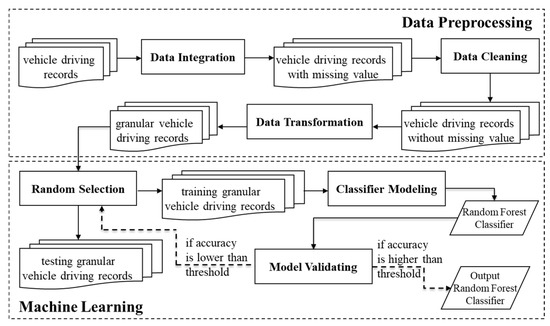
Figure 1.
Work flow of our proposed method.
3.1. Data Preprocessing
In most of the published literature, OBD have been used to collect vehicle driving data for analysis of driving behaviors. For example, Nirmali et al. [10] and Hwang et al. [12] employed OBD to collect vehicle driving data and applied the decision tree classification method and K-means clustering algorithm to analyze the driving behaviors that influenced energy consumption. Their results showed that speed change was a significant influence on energy consumption. In this study, an electric bus, model BYD K9 [16], was chosen as the vehicle type for analysis. The BMS was used to collect vehicle driving data and battery information, as shown in Figure 2. The collected vehicle driving data were integrated, cleaned, transformed for better quality, and prepared for analysis of the eco-driving behaviors.
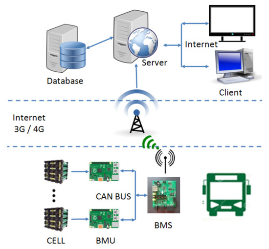
Figure 2.
Data transmission flow of the battery management system (BMS).
3.1.1. Data Integration
We collected the operating data for the EAA-305 electric bus on route 355 in Taichung City. Route 355 is approximately 11.2 km long and starts from the Youyuan-Zhongzhe Intersection to Xiyuan High School, bypassing the Tzu Chiang market. The route mainly consists of flat sections in the downtown area and slow sections adjacent to markets and schools. The passengers are mainly students and housewives and the daily numbers are constant, and therefore the driving behaviors are suitable for energy consumption analysis. The BMS in the electric bus collects the vehicle driving data and returns real-time vehicle information about every 10 s. The data packets are transmitted to the cloud platform via the mobile network and are written into the database. In this study, a backend database was used to collect vehicle driving data. The data were collected between August 2018 and the end of March 2019, with a total of 1,145,053 records. Each data record had a total of 18 fields, as shown in Table 1.

Table 1.
Format of the data collected by the BMS.
3.1.2. Data Cleaning
The original data were reviewed in different dimensions for cleaning in preparation for target analysis. The different dimensions applied to the data cleaning steps are explained as follows:
- Charging information The electric bus has a two-stage starter. In the first state, the power is on, but the motor is idle, and the motor temperature is preset to zero. In this case, the vehicle cannot be driven but only allows the signal handshake between the vehicle controller and the charger during charging. In the second stage, the motor is started, and the bus can be driven. This study focused on analyzing the driving behaviors that influence energy consumption as the vehicle is driven. This required that the charging state data be cleared.
- Time interval The BMS returns vehicle driving data every 10 s. However, the transmission of data is delayed due to the mobile network, creating a greater than 10 s interval in data transmissions. To maintain the consistency of the data trends, the data were cleared when received after a delay of more than 10 s.
A total of 1,145,053 original records were collected during vehicle starts, among which there were 308,826 charging data records that accounted for about 27% of the total original data. After the charging data were cleared, the total number of driving data records was 836,227, among which 75,249 records had a time interval of more than 10 s (accounting for approximately 9% of the driving data). After data cleaning, a total of 760,978 data records remained for analysis. Accordingly, in total, we removed 33.5% meaningless records from the original records ().
3.1.3. Data Transformation
Nirmali [17] and Hwang [18] argued that driving behaviors such as sudden acceleration and slamming on the emergency brakes affected energy consumption. The evaluation indicators related to such behaviors included but were not limited to vehicle speed, motor speed, acceleration, and deceleration. In this study, the acceleration and deceleration calculated using the time interval and vehicle speeds were added as new features to be analyzed. As energy consumption factors for analysis, the driving energy consumption was categorized into three levels, namely low, medium, and high. Before introducing the levels of energy consumption, first, we describe the formal definitions for illustrating the terminologies we used as follows:
Definition 1.
Power Consumption The power consumption refers to the electrical energy per second, supplied to the bus driving. In this study, power consumption is measured in units of kilowatts per second (kWh/s) that can be easily calculated from the data (cumulative driving power consumption and time interval) collected by the BMS.
Definition 2.
Energy Consumption The energy consumption refers to the electrical energy per kilometer supplied to the bus driving. In this study, energy consumption is measured in units of kilowatts per kilometer (kWh/km). The formulation of energy consumption is given by Equation (1) as follows:
where .
According to Lai’s definition [19], the three driving speed levels were low (less than 30 km/h), medium (30 to 50 km/h), and high (greater than 50 km/h), and the average power consumption efficiency of the buses ranged from 0.6411 km/kWh to 1.0172 km/kWh. Here, the term “power consumption efficiency” is the reciprocal of energy consumption, i.e., In Lai’s study [19], the “power consumption efficiency” was also divided into the following three levels: low (less than 0.6 km/kWh), medium (0.7 to 0.9 km/kWh), and high (more than 1 km/kWh). Therefore, in this study, we adopted the same idea to determine the the levels of energy consumption. As a result, we classified the obtained energy consumption into low, medium, and high levels, as shown in Table 2. Energy consumption below 0.1 power consumption (kWh/10 s) was defined as the low level of energy consumption, with a vehicle speed of less than 30 km/h and a power consumption efficiency of more than 1 km/kWh. The medium level of energy consumption was 0.1 power consumption (kWh/10 s), with a vehicle speed of 30 km/h to 50 km/h and a power consumption efficiency of 0.7 km/kWh to 0.9 km/kWh. The high level of energy consumption was above 0.1 power consumption (kWh/10 s), with a vehicle speed of more than 50 km/h and a power consumption efficiency of less than 0.6 km/kWh.
Table 2.
Power consumption analysis.
We analyzed the vehicle operating and driving data collected in this study to calculate the daily mileage and power consumption. We divided the daily mileage by daily power consumption to obtain the daily power consumption efficiency (km/kWh). Figure 3 and Figure 4 show the statistical data of the vehicle speed (km/h) and power consumption efficiency. We can observe that both the distributions of vehicle speed and power consumption efficiency are negatively skewed, which means the average vehicle speed is less than the most frequent vehicle speed, and the average power consumption efficiency is less than the most frequent power consumption efficiency. Therefore, we could realize that the average values of the two variables do not have sufficient representativeness. As a result, using the distribution modes in Figure 3 and Figure 4, we summarized the research vehicle‘s eco-driving indicators; the vehicle speed was 31 km/h, and the power consumption efficiency was 0.73 km/kWh. From the aforementioned data, we verified that the research vehicle’s eco-driving regime fell within the medium energy consumption band and the vehicle speed (km/h) and power consumption efficiency at this level of energy consumption accorded with the optimal driving status.
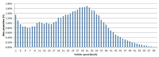
Figure 3.
Distribution of the vehicle speed (km/h) in analytical data.
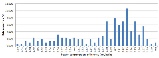
Figure 4.
Distribution of the power consumption efficiency in analytical data.
3.2. Machine Learning
After data preparation, the original data were converted into analytical data, as shown in Table 3. Decision tree and random forest algorithms were employed to construct the analytical models. The analytical data were divided into a training set (80%) and a test set (20%) for model training and prediction. Then, the models were evaluated using indicators such as accuracy, precision, recall, and the F1 score. The optimal models were obtained by adjusting the algorithmic parameters. We constructed models for analyzing driving energy consumption and summarized the factors that influence driving energy consumption to deduce the eco-driving indicators.
Table 3.
Dataset for machine learning.
3.2.1. Modeling
Python is currently the most popular open-source programming language in the field of machine learning [19]. Scikit-learn is an open-source toolkit used with Python that provides many algorithmic functions and focuses on data modeling. With simple and efficient data analysis tools, it is widely used in the field of data analysis [20,21]. In this study, we used Python’s scikit-learn as the data analysis tool for machine learning.
Machine learning’s classification algorithm is categorized as supervised learning, which is suitable for classifying data with clear analytical targets. The decision tree provides graphical analysis to explain and understand the classification rules easily; it is the most widely used classification model in machine learning [22]. Actually, there are various types of decision tree algorithms. Meanwhile, ID3 [23] and C4.5 [24] are the most popular decision tree algorithms for solving classification problems, and CART is the most popular decision tree algorithm for solving regression problems. The main difference between ID3 and C4.5 is the mechanism for dealing with the numerical feature. ID3 directly treats a numerical feature as discrete feature, i.e., every number is treated as a label. On the contrary, C4.5 involves discretization subroutine in the learning algorithm to deal with the discretization of the numerical feature. CART, which is widely applied, uses the Gini coefficient as the feature selection criterion and can be used with classification trees and regression trees. Additionally, CART is characterized by higher operational efficiency and accuracy than ID3 and C4.5. The random forest model formed by integrated learning based on decision trees [25] can effectively reduce the error rate of the decision tree model and solve the overfitting problem [26]. Therefore, we adopted CART, decision tree, and random forest as the classification algorithms for machine learning.
3.2.2. Parameter Adjustment and Model Training
To reduce the impact of randomly divided training and test sets on model evaluation and to improve the model’s accuracy, we combined cross-validation and grid search to find the models’ optimal parameters. The training parameters were set to improve accuracy and reduce overfitting. The model parameters used in this study were as follows:
- Decision tree model parameter The maximum depth of the tree ranged from 1 to 20;
- Random forest model parameters The maximum depth of the tree ranged from 1 to 20 and the trees produced numbered 10 and 100.
The model training is explained in Algorithm 1. We can see that our training strategy follows the manner of cross-validation that is a statistical analysis method used to check the performance of the classifier. This method evenly splits the training set into K folds, among which the Kth fold is used as the validation set and the remaining K-1 folds are used as the training set. After K training iterations, the average score of K iterations is used as the validation score. The scoring method combines grid search and cross-validation and executes different parameter combinations in sequence, thus, obtaining all the scores. The parameter combination that scores the highest was regarded to be the optimal model. The purpose of this scoring method is to reduce overfitting a single training set, and thereby obtain a reliable and stable model.
| Algorithm 1: Model Training Algorithm Based on K-Fold Cross-Validation. |
| Input: Granular Vehicle Driving Records Output: Validated Random Forest Classifier 1: Divide Granular Vehicle Driving Records into K folds (for any ) 2: 3: 4: For each in : 5: Set as the test dataset 6: Train a random forest classifier from the remaining dataset 7: Evaluate the random forest classifier on test dataset to produce the accuracy 8: If 9: 10: 11: end if 12: end for 13: return |
3.2.3. Model Prediction and Evaluation
The optimal models obtained after parameter adjustment and training were predicted using the test set. The prediction results, mainly their accuracy, were evaluated. When the predicted accuracy was closer to one or the precision and recall were both high, the analytical model yielded a better result. If between prediction and recall one was low and the other high, the F1 score was used for comprehensive evaluation. The classification indicators for evaluation are described as follows:
- Accuracy The proportion of correctly classified samples in total samples;
- Precision The proportion of samples with the real value being positive among the total samples when the predicted value was positive and corresponded to the precision of retrieval;
- Recall The proportion of samples with the predicted value being positive among the total samples when the real value was positive and corresponded to the recall ratio of retrieval;
- F1 score The harmonic mean of precision and recall, which was a comprehensive evaluation criterion used to evaluate the robustness of the model.
3.2.4. Model Analysis
The decision tree analytical model can produce a tree structure through visualization in which the paths from the root node to each child node represent classification rules. The paths in the structure diagram are organized into a collection of classification rules. The classification rules can be summarized to obtain the correlation between classification targets and data features. In this study, the random forest model was used to analyze the features influencing energy consumption, and then the classification rules of the decision tree model were evaluated to deduce the eco-driving indicators.
4. Results
4.1. Model Evaluation
In this study, the grid search was combined with five-fold cross-validation to adjust the model parameters for training. The classification indicators for each parameter combination were evaluated within the specified parameter range to construct optimal models for subsequent model analysis.
4.1.1. Decision Tree
The maximum depth of the decision tree was chosen as the parameter to be adjusted. The scoring results of the classification indicators for each parameter value were converted into bar charts to interpret their trends, as shown in Figure 5. The accuracy score started to exceed 0.8 at a depth of 5 and then slowly increased until it reached the maximum value of 0.821 at a depth of 11. Thereafter, the accuracy decreased slowly to a score of less than 0.8 at maximum depth. The indicator trends evidenced that all classification indicators scored the best at a maximum depth of 11. The comprehensive evaluation results showed that this parameter, namely the maximum depth of the tree, was optimal when it was 11. The optimal parameter was brought into the model test for target prediction, and the prediction results were presented using a confusion matrix and receiver operating characteristic (ROC) curves (Figure 6) to verify that the model was optimal. The model validation process was as follows:
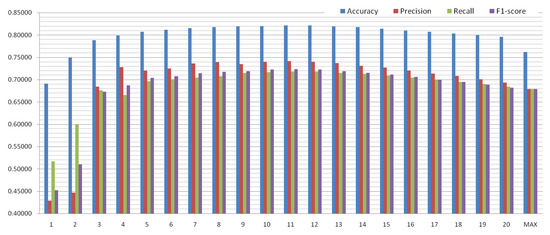
Figure 5.
Evaluation indicators of the decision tree.
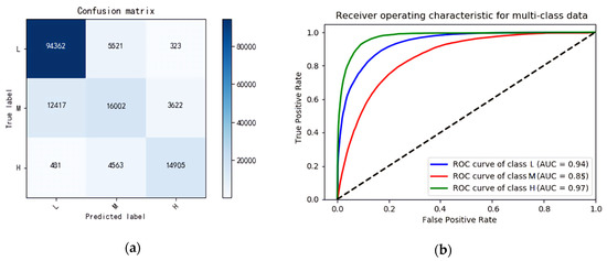
Figure 6.
(a) Confusion matrix of the decision tree; (b) Receiver operating characteristic (ROC) curves of the decision tree.
- Grid search The parameter, namely the maximum depth of the tree, was optimal when it was 11. In this case, the model accuracy was 0.821.
- Confusion matrix The validation results of the indicators for each power consumption level are presented in Table 4. The indicators of low and high energy consumption scored higher, showing that the analytical model had better classification effects in terms of low and high energy consumption.
Table 4. Validation results of the indicators in the optimal decision tree model.
- ROC curve For medium energy consumption, the area under the curve (AUC) was 0.85, showing that the model had good discrimination. For both low and high energy consumption, the AUC was greater than 0.9, confirming that the model had excellent discrimination. Overall, the model had clear discrimination for all power consumption levels.
4.1.2. Random Forest
The number of trees generated by the random forest and the maximum depth of the trees were chosen as parameters to be adjusted. The scoring results of the classification indicators for each parameter value were converted into bar charts to interpret their trends, as shown in Figure 7. The accuracy score started to exceed 0.8 at a depth of 3, and then slowly increased. If the number of trees generated was 10, a maximum accuracy of 0.828 was achieved at a depth of 14. If the number of trees generated was 100, a maximum accuracy of 0.832 was achieved at a depth of 18. Thereafter, the accuracy slowly decreased until it remained higher than 0.8 at a depth of 20. The indicator trends confirmed that the accuracy and F1 scores were best when the number of trees generated was 100 and the depth was 18. The comprehensive evaluation results showed that the parameters were optimal in this case. The optimal parameters were brought into the model test for target prediction, and the prediction results were presented using a confusion matrix and ROC curves (Figure 8) to verify that the model was optimal. The model validation process was as follows:
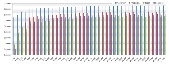
Figure 7.
Evaluation indicators of the random forest.
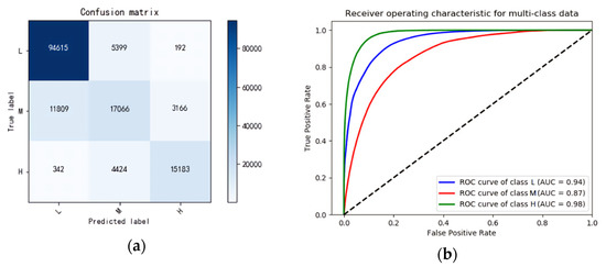
Figure 8.
(a) Confusion matrix of the random forest; (b) ROC curves of the random forest.
- Grid search The parameters were optimal when the number of generated trees was 100 and the depth was 18. In this case, the model accuracy was 0.832.
- Confusion matrix The validation results of the indicators for each power consumption level are presented in Table 5. The indicators of low and high energy consumption scored higher, showing that the analytical model had better classification effects in terms of low and high energy consumption.
Table 5. Validation results of the indicators in the optimal random forest model.
- ROC curve For medium energy consumption, the AUC was 0.87, showing that the model had good discrimination. For both low and high energy consumption, AUC was greater than 0.9, confirming that the model had excellent discrimination. Overall, the model had clear discrimination for all power consumption levels.
4.1.3. Summary
Table 6 shows the effectiveness of decision tree and random forest. Although the concept of decision tree is similar to that of random forest, random forest involves the idea of ensemble learning, and therefore random forest usually outperforms decision tree. Thus, we reveal the effectiveness of decision tree and random forest and also show how much improvement random forest can achieve as compared with decision tree, as shown in Table 6. We can observe that random forest can achieve about 4–5% improvement rate in terms of precision. However, the decision rules of random forest are much more complicated than those of decision tree. Since the interpretability is important for applying the learned model in a real-world approach, it is reasonable to trade such slight improvement for the significant interpretability. Furthermore, the comprehensive evaluation yields the following two conclusions:
Table 6.
Comparison between the optimal decision tree and random forest models.
- Overall score The random forest model was superior to the decision tree model across all four indicators, leading us to conclude that the random forest model was the optimal analytical model for eco-driving.
- Scores for each energy consumption level The scores of the indicators of low and high energy consumption were better leading to the conclusion that the model clearly discriminated the classification effects of low and high energy consumption.
4.2. Model Analysis
The optimal decision tree and random forest models were analyzed to summarize the features influencing driving energy consumption. According to the decision tree classification rules and the random forest feature weights, the eco-driving indicators were comprehensively evaluated.
4.2.1. Feature Weights
The feature weights of the optimal random forest model are shown in Figure 9. The features with weights that were higher than 0.1 were regarded to be the factors that influence driving energy consumption. The energy consumption factors included features such as vehicle speed, motor speed, and total voltage. The feature trends of power consumption being reduced were evaluated as follows:
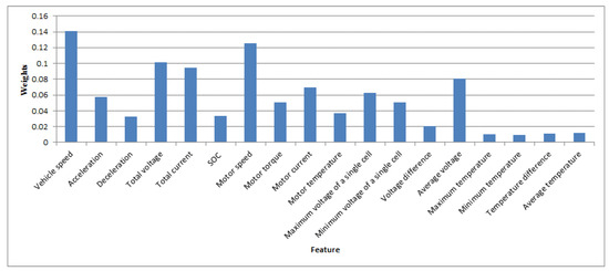
Figure 9.
Feature weights of the optimal random forest model.
- Vehicle speed The lower the vehicle speed, the lower the motor output power. In this case, the current consumption would be lower if the voltage was constant;
- Motor speed The lower the motor speed, the lower the motor output power. In this case, the current consumption would be lower if the voltage was constant;
- Total voltage The higher the total voltage, the lower the current consumption if the power was constant.
4.2.2. Classification Rules
On the basis of the data, eight classification rules were obtained according to the energy consumption levels, as shown in Table 7. In the above analysis, the classification rules were summarized according to the feature weights. In this study, the energy-saving feature trends were evaluated. The lowest vehicle speed, motor speed, and the highest total voltage were used as the deduction criteria.
Table 7.
Classification rules of the optimal decision tree model.
According to the energy-saving feature trends, we deduced the driving indicators for different power consumption levels as follows:
- Low energy consumption (deduction from Rules 1, 2, and 3) The motor speed was below 425.5 rpm, or the total voltage exceeded 560.15 V;
- Medium energy consumption (deduction from Rules 4, 5, and 6) The motor speed ranged from 425.5 rpm to 779.5 rpm, or the total voltage ranged from 560.15 V to 549.25 V;
- High energy consumption (deduction from Rules 7 and 8) The motor speed exceeded 779.5 rpm, or the total voltage fell below 549.25 V.
The purpose of this study was to deduce applicable eco-driving indicators. From using the driving indicators for different energy consumption levels, we inferred the following:
- Driving indicators for both low and medium power consumption The motor speed was below 779.5 rpm, or the total voltage exceeded 549.25 V;
- Driving indicators for nonhigh power consumption The motor speed was below 779.5 rpm, or the total voltage exceeded 549.25 V.
According to the above inferences, we verified the optimal eco-driving indicators, that is, the motor speed was below 779.5 rpm, or the total voltage exceeded 549.25 V.
4.2.3. Summary
This section describes the evaluation of the decision tree and random forest analytical models. The eco-driving indicators were summarized using feature weights and classification rules as follows:
- Feature trend From the random forest analytical model, we inferred that the vehicle speed, motor speed, and total voltage had a significant impact on driving energy consumption. The energy-saving feature trend derived from the electric power equation was that the lower the vehicle speed, the lower the motor speed, and the higher the total voltage.
- Driving indicators We summarized the energy consumption indicators based on the decision tree classification rules. Through cross-validation between indicators of medium and low energy consumption and indicators of nonhigh energy consumption, we deduced the optimal eco-driving indicators to be motor speeds below 779.5 rpm or the total voltage exceeding 549.25 V.
5. Case Study
5.1. Operational Benefits
We collected the driving data from real-time vehicle operations. On the basis of the statistics, the average daily power consumption efficiency of the vehicle was 0.67 km/kWh. The average daily energy efficiency of this vehicle at medium power consumption was 0.73 km/kWh. It can be seen that the power consumption efficiency of this vehicle falls in the high energy consumption band. Eco-driving, as defined in this study, falls in the medium energy consumption band, thereby effectively improving the power consumption efficiency and operational benefits. This section provides operating data statistics such as the monthly mileage, driving energy consumption, and power consumption efficiency, as shown in Table 8. We can see from the indicators for evaluating the operational benefits that longer mileages or higher power consumption efficiencies help to save energy and reduce carbon emissions as well as driving costs. The three evaluation indicators were power consumption, carbon emission, and driving cost. The formal definitions of carbon emissions and driving cost are given as follows:
Table 8.
Statistics on the monthly mileage and power consumption in operating data.
Definition 3.
Carbon Emission The carbon emission refers to total carbon-containing gases emissions caused by the electronic buses. In this study, carbon emission is measured in units of kilogram (kg). The formulation of carbon emission is given by Equation (2) as follows:
Definition 4.
Driving Cost The driving cost refers to the financial cost per kilometer caused by the electronic buses. In this study driving cost is measured in units of new Taiwan dollars per kilometer (NTD/km). The formulation of driving cost is given by Equation (3) as follows:
From the operating statistics in Table 8, we note that the monthly mileage was approximately 3955 km, and the average monthly power consumption efficiency was 0.67 km/kWh. The eco-driving standards obtained in this study are expected to improve the power consumption efficiency to 0.73 km/kWh. The correlation coefficients of Taiwan Power Company are as follows: the carbon emission was 0.554 kg/kWh [1] and the average electricity price was 2.6253 NTD/kWh [27]. The indicators for evaluating operating data and eco-driving were calculated as follows:
- Operating data (power consumption efficiency = 0.67):
- Monthly power consumption, 3955/0.67 = 5903 (kWh);
- Carbon emissions, 5903 × 0.554 = 3270 (kg);
- Driving cost, 2.6253/0.67 = 3.9 (NTD/km).
- Eco-driving (power consumption efficiency = 0.73):
- Monthly power consumption, 3955/0.73 = 5418 (kWh);
- Carbon emissions, 5418/0.554 = 3002 (kg);
- Driving cost, 2.6253/0.73 = 3.6 (NTD/km).
According to the above evaluation indicators, eco-driving can improve the monthly operational improvements of each vehicle as follows:
- Energy saving Energy consumption was reduced from 5903 kWh to 5418 kWh (by 485 kWh), increasing the benefit by about 8.2%;
- Carbon reduction Carbon emissions were reduced from 3270 kg to 3002 kg (by 268 kg), increasing the benefit by about 8.2%;
- Operation The driving cost was reduced from 3.9 NTD/km to 3.6 NTD/km, saving 0.3 NTD/km.
Before we demonstrate the statistics on monthly mileage and power consumption in operating data, we formally define the terms “energy consumption” and “power consumption”.
In this study, energy savings, carbon reduction, and driving energy consumption were the indicators used to evaluate the operational benefits. When the power consumption efficiency increased, the benefits of energy saving and carbon reduction would be improved. The greater the mileage, the less the driving cost. This section concludes that the eco-driving of the research vehicles could improve energy savings and carbon reduction by 8.2% and reduce the monthly driving cost by NTD 1187.
5.2. Discussion
In this study, analytical models were constructed based on the driving data of an EAA-305 electric bus on route 355. As described in this section, the data from different vehicles and different routes were collected for model validation to evaluate the general applicability of the analytical models proposed in this study. The driving conditions of two routes, namely route 352 and route 355, were analyzed. Route 355, 11.2 km long, passes by schools and markets in the downtown area and has more flat stretches and traffic lights, resulting in a lower and more variable driving speed on this route. Route 352, 21.1 km long, stretches along the Dadu Plateau to the downtown area of Taichung City and has a gentle upward slope and fewer traffic lights, so the driving speed on this route is higher and more consistent. Driving data from buses, EAA-301 on route 355 and EAA-592 on route 352, were collected, both of which were electric vehicles of the same model as bus EAA-305 in this study. The data from the two vehicles were collected from August 2018 to the end of March 2019, which corresponded with that of EAA-305 and this study’s analytical models were compared in two schemes, namely Scheme A and Scheme B as follows:
- This study EAA-305 electric bus on route 355;
- Scheme A A different vehicle on the same route, that is, electric bus EAA-301 on route 355;
- Scheme B A different vehicle on a different route, that is, electric bus EAA-592 on route 352.
We input the data of the two schemes into the analytical models. The evaluation results of the classification indicators are presented in Table 9. We found that the scores for Scheme A were closer to those of the analytical models used in this study, whereas the F1 score for Scheme B differed significantly from that of the other analytical models applied. Therefore, we concluded that the energy consumption classification for Scheme B was not suitable. Figure 10 shows the comparative distribution of speed and energy consumption in Schemes A and B in this study. From Figure 10a, we observed that the vehicle speeds in this study and Scheme A ranged from 21 to 30 km/h, whereas the vehicle speeds in Scheme B ranged between 31 km/h and 40 km/h. According to the analysis of the vehicle speed and power consumption efficiency in Table 2, medium energy consumption in this study and Scheme A ranged between 0.06 kWh and 0.12 kWh, whereas in Scheme B, it was 0.10–0.16 kWh. We analyzed the analytical models’ power consumption classification methods by considering the power consumption ranges mentioned above and the proportion of driving energy consumption data in Figure 10b. The analysis results showed that this study had the same energy consumption classification as Scheme A, and their data proportions were both approximately 20%; the medium energy consumption of Scheme B was changed to 0.1–0.2 kWh, and its data proportion was increased from 12.5% to 18.5%. Figure 11 shows the evaluation results of the factors which had feature weights higher than 0.1 that influenced energy consumption. The vehicle speed, motor speed, and total voltage were the factors influencing energy consumption in this study and Scheme A, whereas the motor speed and total current were the influencing factors in Scheme B. The comprehensive evaluation results showed that the influencing factors in this study and Scheme A were the same, and consequently, identical analytical models could be constructed for them; the influencing factors in Scheme B differed from this study, and therefore required the construction of different analytical models.
Table 9.
Statistics of classification indicators of various schemes in the case study.
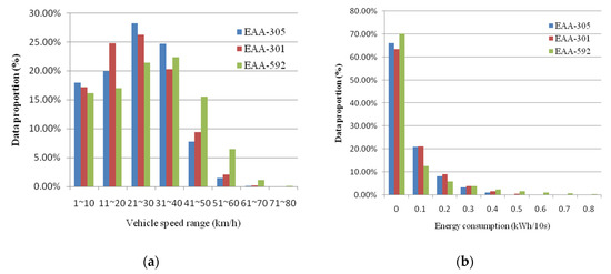
Figure 10.
(a) Vehicle speed distribution of each scheme in the case study; (b) Power consumption distribution of each scheme in the case study.
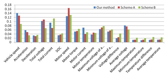
Figure 11.
Feature weights of different schemes in the case study.
According to the above evaluation, we combined the data of this study and Scheme A to construct analytical models for route 355 and constructed additional analytical models for route 352. The analytical models were verified as follows:
- Classification indicators The indicator scores in each analytical model are presented in Table 10. The scores of the analytical models for route 355 lay between those for this study and Scheme A, demonstrating that their classifications did not differ greatly. Both the accuracy and F1 score of the analytical models for route 352 were improved, indicating that the models with adjusted energy consumption classifications performed better.
Table 10. Classification indicators of each model in the case study.
- Feature weights The factors influencing energy consumption in each analytical model are given in Table 11. In the analytical models for route 355, the vehicle speed, motor speed, and total voltage were the factors influencing energy consumption. The influencing factors were the motor speed and motor temperature in the analytical models for route 352.
Table 11. Feature weights of each model in the case study.
- Driving indicators The classification rules of each analytical model are listed in Table 12 and Table 13. We summarized the indicators for each analytical model based on the above features. For the analytical models for route 355, eco-driving required a motor speed below 773.5 or a total voltage higher than 549.75. For the analytical models, for route 352, eco-driving required a motor speed below 1140.5, a total voltage higher than 545.45, or a motor temperature below 52.5.
Table 12. Classification rules of route 355 in the case study.
Table 13. Classification rules of route 352 in the case study.
We can see from the above evaluation and verification that the classification indicators and driving indicators of the same route differed slightly; the energy consumption classification and feature weights should be evaluated for different routes. Route 352 is longer and the driving speed on this route is higher and more constant, resulting in higher motor speeds. Therefore, it is recommended to construct different analytical models for Scheme B to summarize the driving indicators. We can draw the following conclusions from the above summaries:
- For vehicles on the same route, the same analytical models apply;
- For vehicles on different routes, different analytical models should be constructed.
6. Conclusions
In this study, first, we used a BMS to collect vehicle driving data, then, applied machine learning methods to construct analytical models of energy consumption while driving, and finally deduced eco-driving indicators. The purpose of this study was to provide these deduced eco-driving indicators for performance management by passenger transport operators and for the education and training of drivers, to improve the benefits of energy-saving and carbon reduction, and to save on operating costs. To do so, we adopt the notion of the interpretable modeling which precisely classifies driving behavior and also provides in-depth analysis about the relation between driving behavior and energy consumption. To realize the interpretable modeling, decision tree and random forest models are learned from the collected vehicle driving data. Through the learned interpretable models, we found two eco-driving behaviors. One behaviour is that the driver should maintain the vehicle speed and pedal pressure during driving to keep the speed below 779.5. The other behaviour is that the driver should monitor the battery status while driving, when the total voltage is lower than 549.25, the driver should return to the charging station to charge the vehicle. Accordingly, two benefits of eco-driving in this study were analyzed. One benefit is that improved power consumption efficiency increases the energy-conserving and carbon-reduction benefits, which can reduce the carbon footprint of operations consistently with environmental protection objectives. The second benefit is the saving from reduced costs per kilometer, which can control the operating costs and render the electric bus more economical. For future works, we plan to modify our proposed machine learning method such that the learning process could be performed on an on-vehicle computer, and therefore the model could be trained on an on-vehicle computer such that the all data in the on-vehicle computer could be utilized for training the classifier. In addition, another future research direction should be to involve other traffic-related data for precise analysis. Accordingly, we would try to collect the geographic data for analyzing interaction between eco-driving parameters and the geo-conditions of the route. We would also collect E-ticket data for analyzing interactions between eco-driving parameters and the number of passengers.
Author Contributions
K.-C.L. initialed the idea, addressed whole issues in the manuscript and wrote the manuscript. C.-N.L. implemented algorithms. Finally, J.J.-C.Y. revised and polished the final edition manuscript. All authors have read and agreed to the published version of the manuscript.
Funding
This research was funded by the Ministry of Science and Technology of Taiwan, R.O.C., grant number MOST 109-2221-E-005-057-MY2.
Conflicts of Interest
The authors declare no conflict of interest.
References
- Bureau of Energy, Ministry of Economic Affairs 2020. 2019 Energy Statistical Annual Reports in Taiwan. Available online: https://www.moeaboe.gov.tw/ECW/english/content/ContentLink.aspx?menu_id=1540 (accessed on 31 August 2020).
- Li, M.-Y. Electric Vehicles Are a Better Choice in Taiwan. Sci. Am. 2011, 107. Available online: http://sa.ylib.com/MagArticle.aspx?Unit=featurearticles&id=1712 (accessed on 31 August 2020).
- Beckers, C.J.J.; Besselink, I.J.M.; Frints, J.J.M.; Nijmeijer, H. Energy consumption prediction for electric city buses. In Proceedings of the 13th ITS European Congress, Brainport, The Netherlands, 3–6 June 2019; pp. 3–6. [Google Scholar]
- Wang, J.; Besselink, I.; Nijmeijer, H. Battery electric vehicle energy consumption modelling for range estimation. Int. J. Electr. Hybrid Veh. 2017, 9, 79–102. [Google Scholar] [CrossRef]
- Gallet, M.; Massier, T.; Hamacher, T. Estimation of the energy demand of electric buses based on real-world data for large-scale public transport networks. Appl. Energy 2018, 230, 344–356. [Google Scholar] [CrossRef]
- De Cauwer, C.; Van Mierlo, J.; Coosemans, T. Energy Consumption Prediction for Electric Vehicles Based on Real-World Data. Energies 2015, 8, 8573–8593. [Google Scholar] [CrossRef]
- Haq, I.N.; Leksono, E.; Iqbal, M.; Sodami, F.N.; Kurniadi, D.; Yuliarto, B. Development of battery management system for cell monitoring and protection. In Proceedings of the 2014 International Conference on Electrical Engineering and Computer Science (ICEECS), Sanur-Bali, Indonesia, 24–25 November 2014; pp. 203–208. [Google Scholar]
- Buccolini, L.; Ricci, A.; Scavongelli, C.; DeMaso-Gentile, G.; Orcioni, S.; Conti, M. Battery Management System (BMS) simulation environment for electric vehicles. In Proceedings of the IEEE 16th International Conference on Environment and Electrical Engineering (EEEIC), Florence, Italy, 7–10 June 2016; pp. 1–6. [Google Scholar]
- Lu, L.; Han, X.; Li, J.; Hua, J.; Ouyang, M. A review on the key issues for lithium-ion battery management in electric vehicles. J. Power Sources 2013, 226, 272–288. [Google Scholar] [CrossRef]
- Berckmans, G.; Messagie, M.; Smekens, J.; Omar, N.; Vanhaverbeke, L.; Van Mierlo, J. Cost projection of state of the art lithium-ion batteries for electric vehicles up to 2030. Energies 2017, 10, 1314. [Google Scholar] [CrossRef]
- Vepsäläinen, J.; Kivekäs, K.; Otto, K.; Lajunen, A.; Tammi, K. Development and validation of energy demand uncertainty model for electric city buses. Transp. Res. Part D Transp. Environ. 2018, 63, 347–361. [Google Scholar] [CrossRef]
- Pamuła, T.; Pamuła, W. Estimation of the Energy Consumption of Battery Electric Buses for Public Transport Networks Using Real-World Data and Deep Learning. Energies 2020, 13, 2340. [Google Scholar] [CrossRef]
- Asaithambi, S.P.R.; Venkatraman, R.; Venkatraman, S. MOBDA: Microservice-Oriented Big Data Architecture for Smart City Transport Systems. Big Data Cogn. Comput. 2020, 4, 17. [Google Scholar] [CrossRef]
- Gao, Y.; Guo, S.; Ren, J.; Zhao, Z.; Ehsan, A.; Zheng, Y. An Electric Bus Power Consumption Model and Optimization of Charging Scheduling Concerning Multi-External Factors. Energies 2018, 11, 2060. [Google Scholar] [CrossRef]
- Ping, P.; Qin, W.; Xu, Y.; Miyajima, C.; Takeda, K. Impact of Driver Behavior on Fuel Consumption: Classification, Evaluation and Prediction Using Machine Learning. IEEE Access 2019, 7, 78515–78532. [Google Scholar] [CrossRef]
- BYD K9 Electric Bus. 2020. Available online: https://en.wikipedia.org/wiki/BYD_K9 (accessed on 31 August 2020).
- Nirmali, B.; Wickramasinghe, S.; Munasinghe, T.; Amalraj, C.R.J.; Bandara, H.D. Vehicular data acquisition and analytics system for real-time driver behavior monitoring and anomaly detection. In Proceedings of the 2017 IEEE International Conference on Industrial and Information Systems (ICIIS), Peradeniya, Sri Lanka, 15–16 December 2017; pp. 1–6. [Google Scholar]
- Hwang, C.P.; Chen, M.S.; Shih, C.M.; Chen, H.Y.; Liu, W.K. Apply Scikit-Learn in Python to Analyze Driver Behavior Based on OBD Data. In Proceedings of the 32nd International Conference on Advanced Information Networking and Applications Workshops (WAINA), Krakow, Poland, 16–18 May 2018; pp. 636–639. [Google Scholar]
- Lai, W.-T. An Analysis of Operational Benchmarks, Financial Benefits and Development Strategies for Electric Urban Buses. Transp. Plan. J. 2017, 46, 377–397. [Google Scholar]
- Chen, T.; Guestrin, C. XGBoost: A Scalable Tree Boosting System. In Proceedings of the 22nd ACM SIGKDD International Conference on Knowledge Discovery and Data Mining (KDD ’16); Association for Computing Machinery: New York, NY, USA, 2016; pp. 785–794. [Google Scholar]
- Diaz-Uriarte, R.; Alvarez, S. Gene selection and classification of microarray data using random forest. BMC Bioinform. 2006, 7, 3. [Google Scholar] [CrossRef] [PubMed]
- Pedregosa, F.; Varoquaux, G.; Gramfort, A.; Michel, V.; Thirion, B.; Grisel, O.; Vanderplas, J. Scikit-learn: Machine learning in Python. J. Mach. Learn. Res. 2011, 12, 2825–2830. [Google Scholar]
- Quinlan, J.R. Induction of Decision Trees. Mach. Learn. 1986, 1, 81–106. [Google Scholar] [CrossRef]
- Quinlan, J.R. C4.5: Programs for Machine Learning; Morgan Kaufmann Publishers: Burlington, MA, USA, 1993. [Google Scholar]
- Han, J.; Pei, J.; Kamber, M. Data Mining: Concepts and Techniques; Elsevier: Amsterdam, The Netherlands, 2011. [Google Scholar]
- Breiman, L. Random forests. Mach. Learn. 2001, 45, 5–32. [Google Scholar] [CrossRef]
- Taiwan Power Company. Calculation Table of Average Electricity Price per kWh Submitted to the Electricity Price Commission in the Second Half of 2018. Available online: https://www.taipower.com.tw/tc/page.aspx?mid=1438 (accessed on 31 August 2020).
© 2020 by the authors. Licensee MDPI, Basel, Switzerland. This article is an open access article distributed under the terms and conditions of the Creative Commons Attribution (CC BY) license (http://creativecommons.org/licenses/by/4.0/).