Interval-Based LDA Algorithm for Electrocardiograms for Individual Verification

Abstract

This paper presents an interval-based LDA (Linear Discriminant Analysis) algorithm for individual verification using ECG (Electrocardiogram). In this algorithm, at first, unwanted noise and power-line interference are removed from the ECG signal. Then, the autocorrelation profile (ACP) of the ECG signal, which is a mathematical representation of the degree of similarity between a given time series and a lagged version of itself over successive time intervals, is calculated. Finally, the interval-based LDA algorithm is applied to extract unique individual feature vectors that represent distance and angle characteristics on short ACP segments. These feature vectors are used during the processes of enrollment and verification of individual identification. To validate our algorithm, we conducted experiments using the MIT-BIH ECG and achieved EERs (Equal Error Rate) of 0.143%, showing that the proposed algorithm is practically effective and robust in verifying the individual’s identity.

1. Introduction

Since the invention of electrocardiogram (ECG) recording in 1903 [1], a considerable number of studies using the electrocardiogram have been performed in the fields of diagnosing cardiac-related diseases [2,3,4,5], detecting sleep apnea [6], monitoring driver drowsiness [7], and measuring blood pressure [8], because of its advantage of noninvasive convenience. Recently, researchers started to use the ECG biometrics to verify individual identity [9]. The ECG is a suitable tool because the signal itself constantly changes depending on the sympathetic/parasympathetic activities and it is resistant to attacks and duplication [10,11,12].

According to the latest US Federal Trade Commission report published in March 2019 [13], identity theft and cybercrime ranked third among the issues most complained about. Such kinds of identity fraud and hacking are becoming seriously dangerous. Unfortunately, they are unavoidable as long as we use password-based identity authentication systems. Therefore, new types of biometrics such as facial characteristics [14], gait [15], fingerprints and iris scans [16], vein pattern [17], etc., have been developed. Nevertheless, References [18,19] show that they are still vulnerable to a replay/falsification attack even though they perform better with very low identification errors. To avoid problems related to such attacks, the biometrics should be a variable, so that they cannot be stolen, duplicated, or shared. Thus, many studies are showing a great interest in the ECG signal as a promising alternative biometric [20,21,22,23].

The ECG signal is non-stationary and thus continuously changes over time. The two limbs of the autonomic nervous system (i.e., sympathetic and parasympathetic nerves) are the most important factors determining the changes in the heart rate. This type of variability is called intra-subject variability [24,25,26], that is, the changes occur for the same individual over time. There is also inter-subject variability found in the ECG’s waveform that depends on the position, size, and anatomy of the heart, age, gender, relative body weight, chest configuration, and various other factors [27,28]. Therefore, the ECG signal varies from person to person, implying that we can use it as a biometric for the verification of an individual’s identity.

There have been numerous attempts at applying ECG inter-subject variation for individual verification/identification [20,21,22,23,29,30,31,32], which can be classified into two categories: the fiducial dependent approach [20,21,22,23] and the fiducial independent approach [29,30,31,32]. The fiducial dependent approach relies on local features, such as time duration and amplitude differences between specific points of interest in an ECG, so it is less affected by heart rate variations. However, it has the possibility of missing the overall morphological information that might be useful in identifying individuals. Many studies have focused on fiducial dependent features such as time intervals, angles, and amplitudes between specific fiducial points on the QRS complex [20,33,34,35].

On the contrary, the fiducial independent approach is to find the feature of the ECG signal in the frequency domain rather than the time domain, or to extract the whole morphological features that appear to offer excellent discrimination information among individuals. Many algorithms based on frequency transformation have been proposed for extracting fiducial independent features from ECG signals, in which they use wavelet transform or DCT (Discrete Cosine Transform) to convert ECG signals in the time domain to the frequency domain [36,37,38,39,40]. The autocorrelation method also has been gaining considerable attention because of its excellent performances reported in many studies. It eliminates the need for fiducial point localization in the ECG signal by using an autocorrelation (AC) of the segmented ECG signal followed by DCT or LDA [41,42,43]. More recently, Safie [44] introduced a new feature extraction method, known as Pulse Active Ratio (PAR), that is implemented on electrocardiogram signals for biometric authentication. The Pulse Active Ratio uses pulse width modulation (PWM) to generate new ECG feature vectors and thereby can adapt to changes in heart rate. However, such fiducial independent approaches require tremendous computational effort because the parameters should be generated and compared for every person listed in the database during the verification stage. Furthermore, the database is often updated with intra-subject variability, in which the computational cost increases exponentially as the size of the database increases. This computational cost problem can be mitigated significantly by combining the above-mentioned two approaches.

In this paper, we propose an interval-based Linear Discriminant Analysis (LDA) algorithm, a type of hybrid algorithm that combines the complementary strengths of both fiducial dependent and fiducial independent features, and thereby is able to achieve higher accuracy of identification. The main characteristics of the proposed algorithm are as follows: (i) the use of an autocorrelation profile (ACP) of ECG signal; (ii) the use of short segments of the ACP to extract the interval-based feature vectors, which can be updated every 5 s, showing higher adaptability to intra-subject variation; (iii) the enrollment and verification of the individual’s interval-based feature vectors; and (iv) the update of interval-based feature vectors when the user’s identity claim is accepted.

The remainder of the paper is organized as follows. The proposed LDA algorithm based on the short ACP segments to determine the feature vectors on an interval basis as enrollment process, the verification process, and the algorithm to update the feature vectors are described in Section 2. In Section 3, the experimental results are compared with the existing ECG identification algorithms based on the same public database. Finally, the conclusion is drawn in Section 4.

2. Materials and Methods

The ECG signal reflects the electrical activity of the heart. A basic ECG signal cycle is shown in Figure 1 with a single lead ECG sensor. The signal cycle consists of the P wave, followed by the QRS complex, and the T wave [1,33].

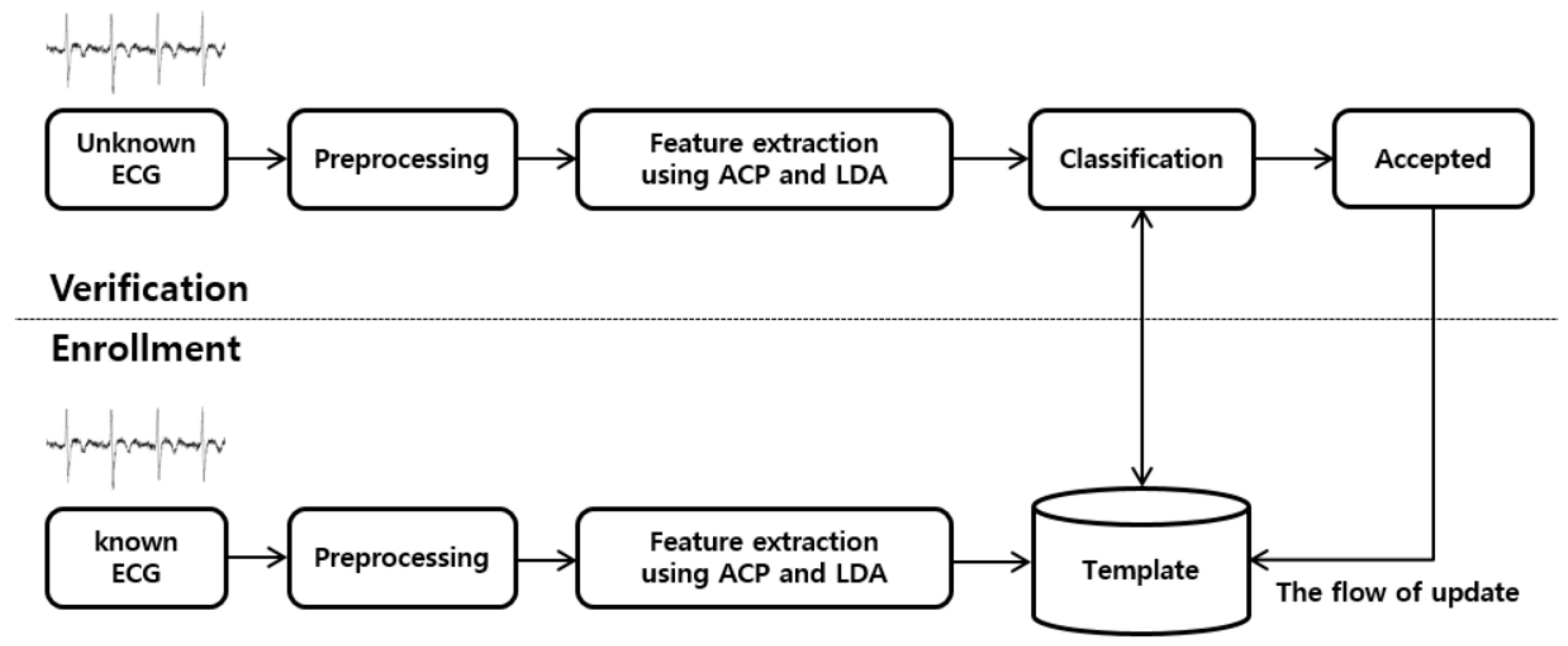
Figure 2 shows a simplified block diagram of the proposed interval-based LDA algorithm. This algorithm mainly consists of signal preprocessing, enrollment, and verification.

In the preprocessing stage, the raw ECG signal’s noise is removed or suppressed. For biometric authentication, every user can use his/her ECG sensor in one of the two operation modes, that is, enrollment or verification mode.

In the enrollment mode/stage, a distinctive feature set is extracted from the ACP (autocorrelation profile) of the ECG on an interval basis to create an association between the user and his/her biometric characteristics. Subsequently, the extracted feature set is stored in a template. This process is called training in the enrollment mode. The template is updated over time, mainly to handle the intra-subject variation of cardiac signals. Longer training of the ECG signal leads to lower chances of false rejection (FR). In this study, the enrollment is performed for 2 min to provide a stable signature.

Similarly, during the verification mode/stage, the newly acquired unknown input is compared with the template stored in the database to verify a claimed identity. The verification decision is made through a matching process based on a feature vector threshold. The obtained matching score is finally compared with the threshold to either accept or reject the target user’s identity claim.

2.1. Preprocessing

We used the ECG data from the MIT-BIH public database to test the proposed algorithm. The MIT-BIH database (MITDB) [34] is the standard ECG database universally used for ECG analyses that contains 48 records of heartbeats collected from 47 subjects; each record was sampled at 360 Hz and is approximately 30 min long. The subjects were 25 men with ages ranging from 32 to 89 years and 22 women with ages ranging from 23 to 89 years. The data were obtained with a two-channel ambulatory Holter monitor at the Bath Israel Deaconess Medical Center from 1975 to 1979. In most database records, the upper signal is a modified limb lead II(MLII) obtained by placing the electrode on the chest, and the lower signal is usually a V1(occasionally V2 or V5 or V4). Normal QRS complexes are usually prominent in the upper signal, thus, we only used the single lead data (the upper signal, MLII) in the experiment.

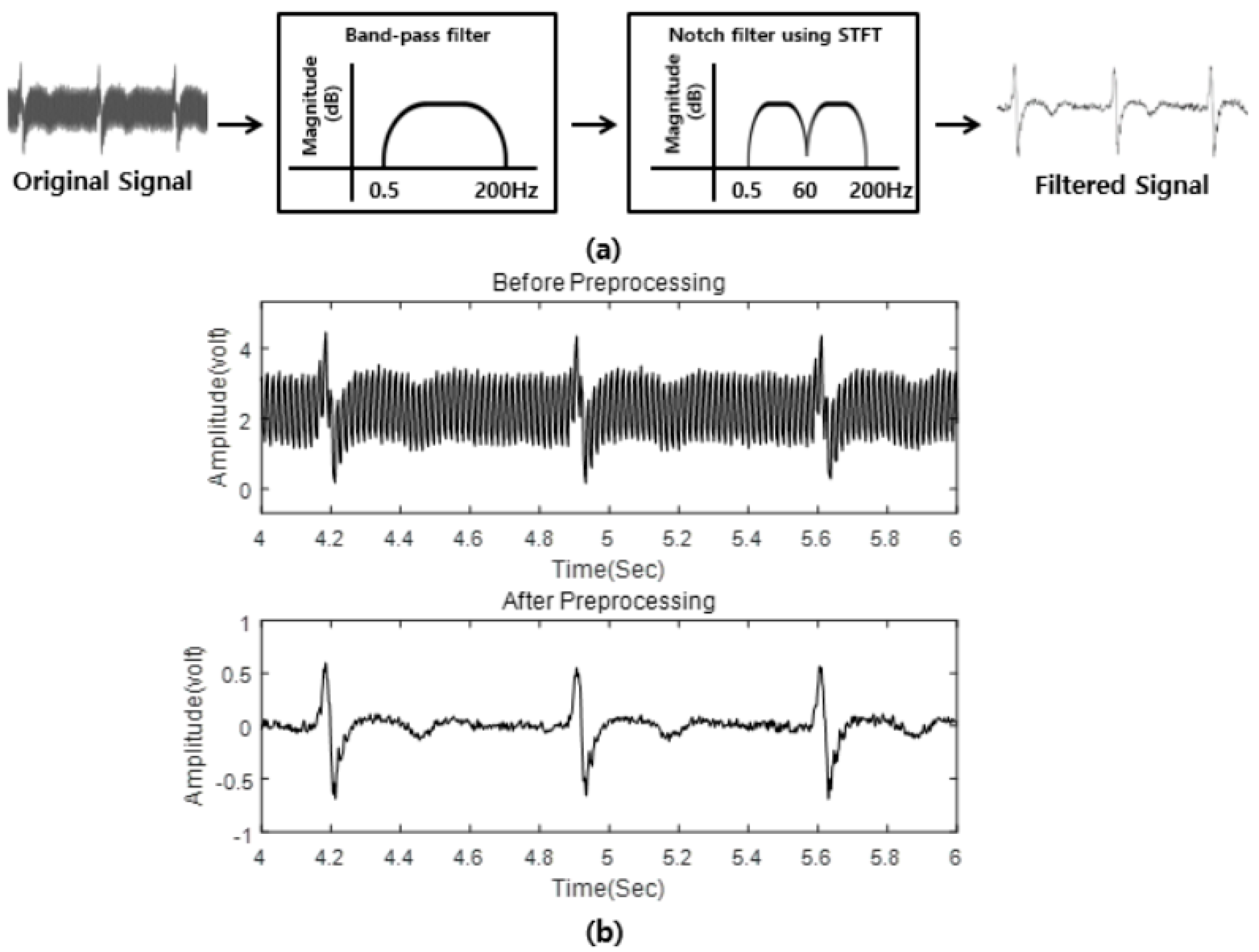
To minimize the negative effect of random noises, we applied the scheme proposed by Sornmo [35] in our study, in which noisy ECG signals are passed through the bandpass filters (BPF) spanning from 0.5 to 200 Hz to reject the DC components and high-frequency noise. Subsequently, we implemented a notch filter and a short-time Fourier transform (STFT) to eliminate the power line interference and its harmonics. Figure 3 shows the preprocessing procedures.

2.2. Feature Extraction

Let the noise-filtered ECG signals be x(n), with the time index n. The proposed method strongly relies on the small pieces of x(n), called classes, and calculates the ACP (autocorrelation profile) of each class. Then, each calculated ACP is sliced into short-time ACP segments; each segment is called ACPlet. By dividing each ACP into multiple ACPlets, we may easily capture the temporal pattern of the ACP in detail. The features we used are mainly based on the amplitude and angle patterns of the ACPlets to identify the similarities between an unknown ACP input and the reference profile.

2.2.1. Calculating the Reference Profile, $\overline{\mathsf{\Phi }}\left(m\right)$

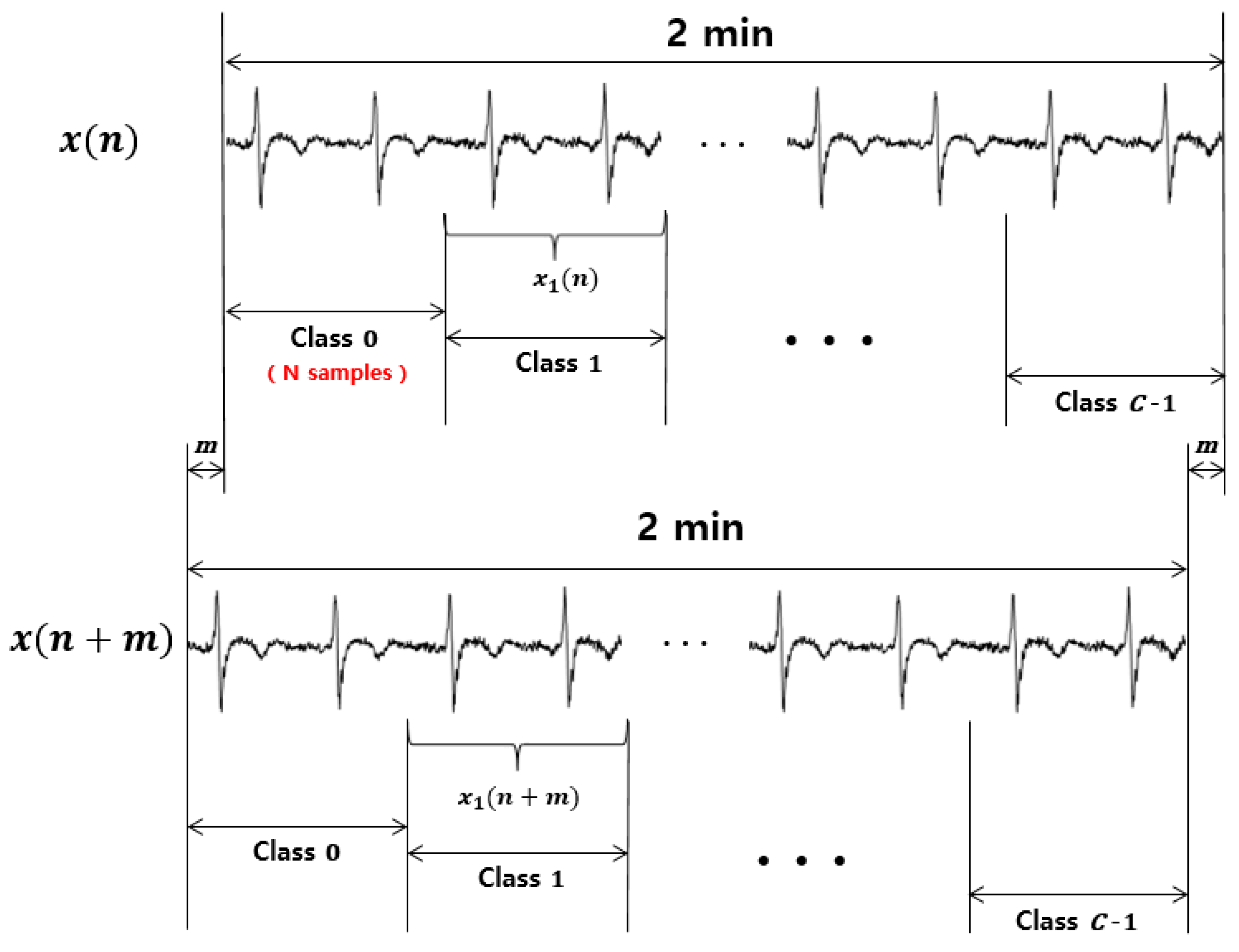
As mentioned in the previous section, during the enrollment mode, 2 min long ECG signals received from the ECG sensor are considered to be the training set x(n). The training set x(n) is then divided into several classes with a length of N. Each class of x(n) is labeled $x_c\left(n\right)$ with the class “c”, as follows

$$x_c\left(n\right)= x\left(n\right)·R_N\left(n-N·c\right) \mathrm{for} \mathrm{a} \mathrm{given} \mathrm{class} c=0,1,\cdots ,C-1$$

(1a)

where

$$R_N\left(n\right)=\{ \begin{array}{c} 1 , 0\le n\le N-1 \\ 0 , \mathrm{otherwise} \end{array}$$

(1b)

Subsequently, the ACP ${\mathsf{\Phi }}_c\left(m\right)$of $x_c\left(n\right)$ can be computed by the following Equation (2a).

$${\mathsf{\Phi }}_c\left(m\right)={\displaystyle {\displaystyle \sum }_{n=0}^{N-1}}{x}_c\left(n\right)·x_c\left(n+m\right) \mathrm{for} 0\le m\le Q-1 \mathrm{and} \mathrm{a} \mathrm{given} \mathrm{class} \mathrm{c}$$

(2a)

where $x\left(n+m\right)$is the time-shifted version of ECG with a time lag m and Q is the length of the QRS complex. Figure 4 shows how the signals $x_c\left(n\right)$ and $x_c\left(n+m\right)$ are defined to obtain the ACP, that is, ${\mathsf{\Phi }}_c\left(m\right)$.

Based on the previous research, the QRS complex is considered to be the most prominent waveform of ECG for individual verification [41,45,46]. Hence, the time shift parameter m of ${\mathsf{\Phi }}_c\left(m\right)$ was chosen between 0 to Q − 1. In this paper, the length Q, which depends on the individual, was calculated using the QRS detection method based on the Pan-Tompkins algorithm [47]. Depending on the individual, the different length of Q helps in achieving a high identification accuracy and robustness of the proposed algorithm.

Based on the assumption that the training set x(n) includes C classes, we define a set of ACPs for C classes as follows:

$${\mathsf{\Phi }}_0\left(m\right),{\mathsf{\Phi }}_1\left(m\right),\cdots ,{\mathsf{\Phi }}_c\left(m\right),\cdots ,{\mathsf{\Phi }}_{C-1}\left(m\right)$$

(2b)

Subsequently, the reference profile $\overline{\mathsf{\Phi }}\left(m\right)$ is defined as the average of all ACPs contained in the training set x(n), given by:

$$\overline{\mathsf{\Phi }}\left(m\right)=\frac{1}{C}{\displaystyle {\displaystyle \sum }_{c=0}^{C-1}}{\mathsf{\Phi }}_c\left(m\right)$$

(3)

where C is the total number of classes in the training set x(n) for 2 min.

2.2.2. Interval-Based Feature Extraction

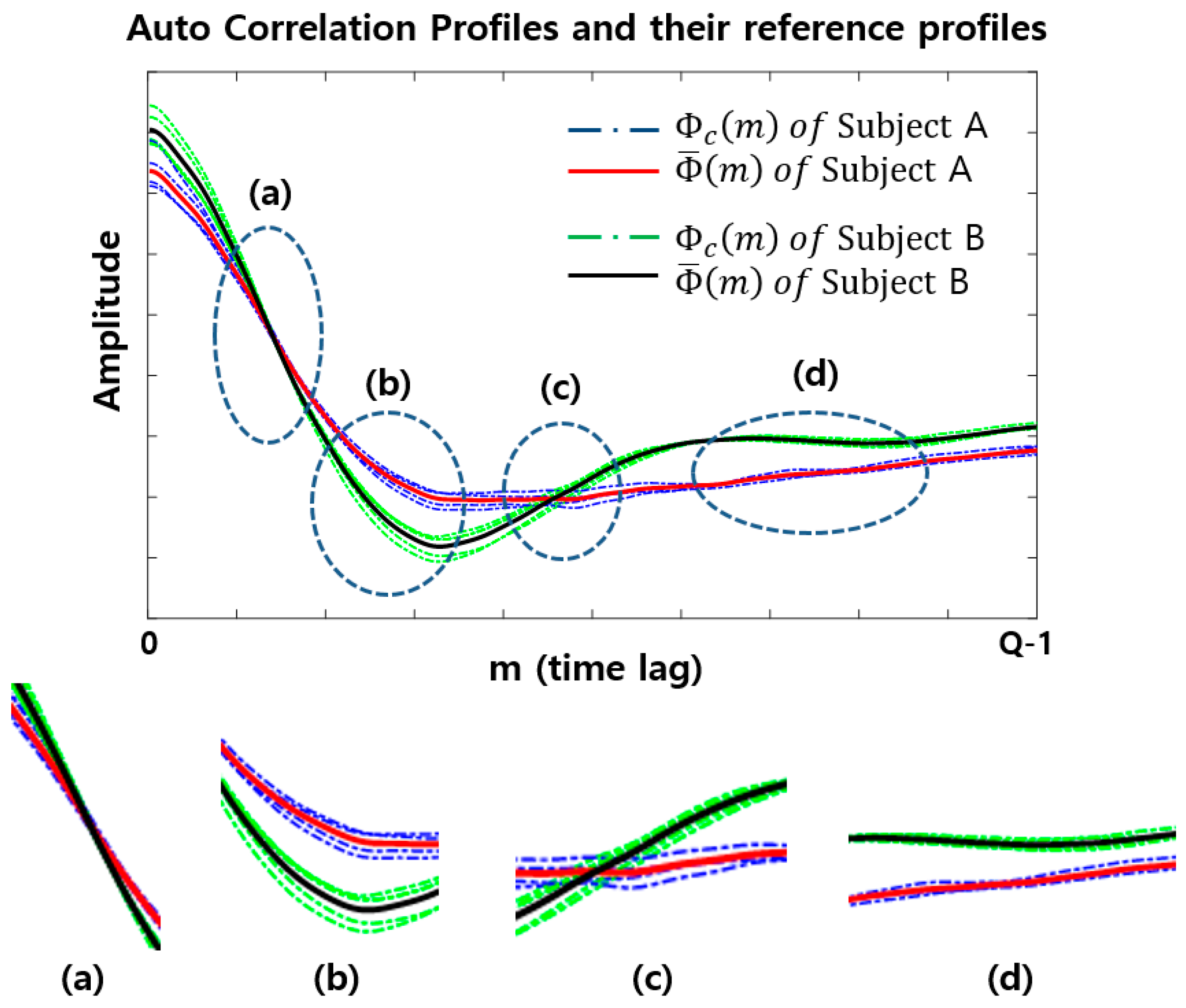
Figure 5 shows an example of ACPs for two different subjects (subject A and subject B). We assumed that each subject has C classes and those C classes are displayed together within the same time period Q.

From Figure 5, the intervals (a) and (c) are when the two subjects are difficult to distinguish by using only the amplitude patterns of ${\mathsf{\Phi }}_c\left(m\right)$, but these two subjects are more easily distinguished using the angle patterns of ${\mathsf{\Phi }}_c\left(m\right)$. It is obvious from the two profiles of (a) and (c) that their angle patterns are significantly different, in which the angle pattern is defined as the angles between the horizontal x-axis and the ACPlet. On the other hand, (b) and (d) are the intervals when the two subjects can be easily distinguished using the amplitude patterns of ${\mathsf{\Phi }}_c\left(m\right)$.

These results lead to the idea of an interval-based feature vector. Accordingly, to facilitate the identification between different subjects, each class needs to be sliced into short-time ACP segments, i.e., the ACPlets. Therefore, in this work, the two features of amplitude and angle patterns of ACP produced for every ACPlet are used to distinguish the ECG signals.

2.2.3. Deciding the Optimal Interval Size for Interval-Based Feature Vector

In Section 2.2.2, we realized that dividing ACPs with a short interval and applying different feature vectors to each ACPlet yields a better identification; however, the interval size should be decided appropriately. The optimal interval size is determined based on the maximum interval that satisfies a mean square error (MSE) criterion between the ACPlets and their linearly fitted lines, such that each ACPlet provides clear angle information.

Based on the assumption of the optimal interval size L, the reference profile $\overline{\mathsf{\Phi }}\left(m\right)$ can be equally divided into Q/L profiles $f_i\left(v\right)$, defined as follows:

$$\overline{\mathsf{\Phi }}\left(m\right)= \left\{ f_1\left(v\right),f_2\left(v\right),\cdots ,f_i\left(v\right),\cdots ,f_{NI}\left(v\right) \right\} \mathrm{for} \mathrm{a} \mathrm{given} L$$

(4)

where i $\left(=\frac{Q}{L}\right)$ is the number of intervals and 0 ≤ ν ≤ L − 1.

Here, let define $\hat{\mathsf{\Phi }}\left(m\right)$ as the set of $g_i\left(v\right)$ that is the $f_i\left(v\right)$ linearly fitted, as follows:

$$\hat{\mathsf{\Phi }}\left(m\right)= \left\{ g_1\left(v\right),g_2\left(v\right),\cdots ,g_i\left(v\right),\cdots ,g_{NI}\left(v\right) \right\}$$

(5)

where 0 ≤ ν ≤ L − 1.

Thus, the optimal interval L is the maximum length that satisfies the following MSE (ζ) criterion between the two profiles $\overline{\mathsf{\Phi }}\left(m\right)$ and $\hat{\mathsf{\Phi }}\left(m\right)$.

$$L=\underset{l}{\max }\left[ {\displaystyle {\displaystyle \sum }_{i=1}^{NI}}{\displaystyle {\displaystyle \sum }_{v=0}^{l-1}}{\left( f_i\left(v\right)-g_i\left(v\right) \right)}^2\le \epsilon \right] \mathrm{for} 2\le l\le \frac{Q}{2}$$

(6)

where ε is the minimum tolerance of the MSE and NI (=Q/L) is the number of intervals. The symbol represented in the above process is illustrated in Figure 6.

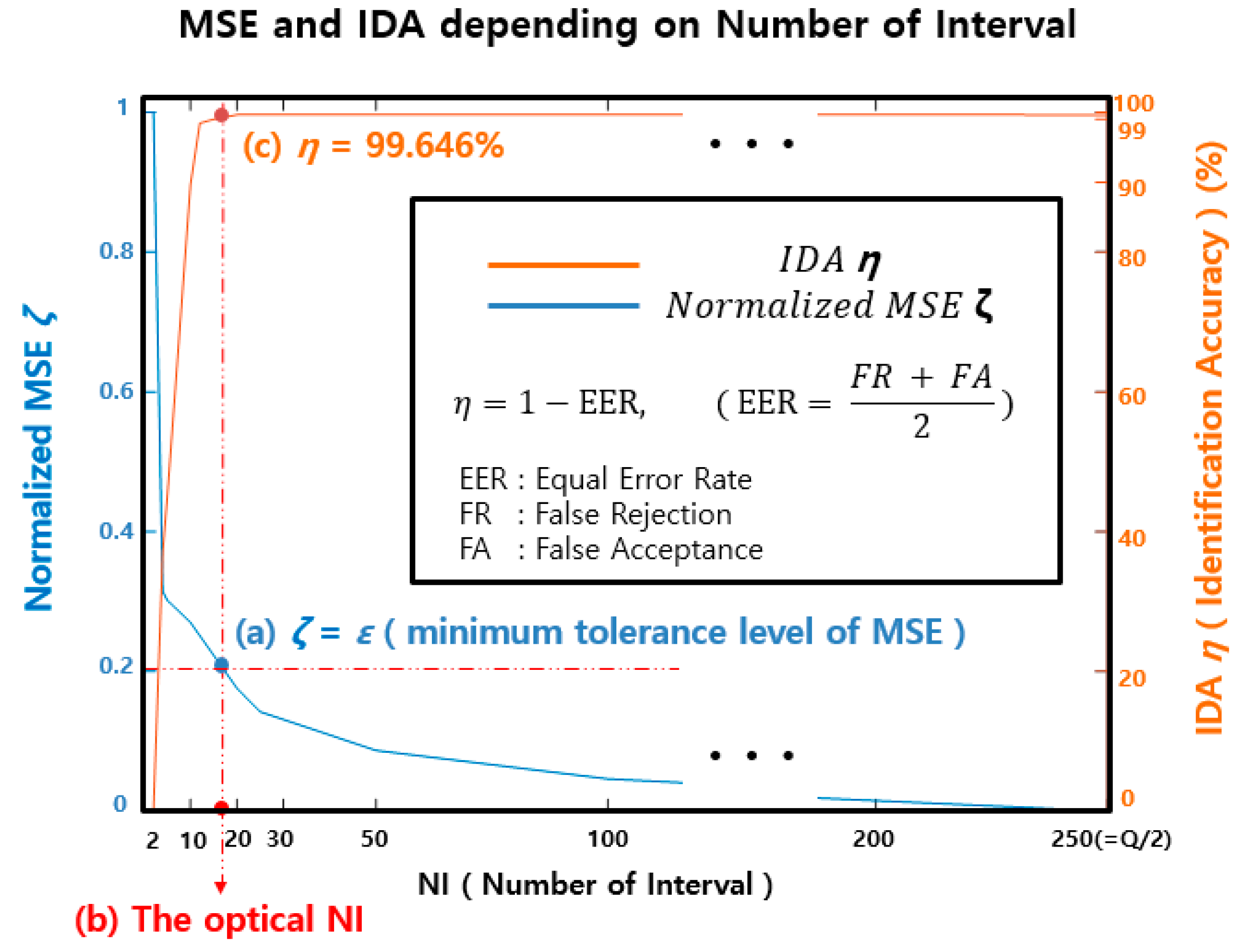
Figure 7 shows typical examples of the MSE ζ and identification accuracy $\eta$ as a function of NI (Number of Interval). In Figure 7, MSE ζ represents the ratio based on the assumption that MSE ζ is 100% when NI is set to 2, where (a) represents the minimum tolerance ε, which is experimentally set to 20%; (b) is the NI value satisfying (a), which corresponds to Q/L; and (c) is the identification accuracy when the NI value corresponds to (b).

The Figure 7 shows that the MSE ζ decreases as NI increases, where a higher NI is proportional to identification accuracy η but requires more computations for the verification process. Accordingly, there is a trade-off between the NI and computational cost. We also observed that the IDA improves with increasing NI; however, the improvement is not significant. For instance, as the NI increases from Q/L to 50, only an improvement of less than 0.2% is obtained. In conclusion, the performance of the proposed algorithm is not highly sensitive to the NI as long as it is greater than Q/L. Finally, the NI is set to Q/L when MSE ζ corresponds to ε, since there is no big difference in the final performance as long as the NI is greater than Q/L.

2.3. Threshold Values for Classification

Our algorithm requires two types of interval-based thresholds for the robust verification of intra-subject variation. One threshold is for the amplitude feature vector and another is for the angle feature vector, denoted $T{H}_{\varphi }\left(i,v\right)$ and $T{H}_{\theta }\left(i\right)$, respectively, where the variable i indicates the interval index. These thresholds are used to check the similarity between the amplitude and angle feature vectors of the newly incoming ACPlets to those stored in the template.

2.3.1. Threshold of Amplitude Similarity: $T{H}_{\varphi }\left(i,v\right)$

Step 1: Consider a subject A for the training set and let define the ACP as ${\varphi }_c^A\left(m\right)$ that consists of the ACPlets ${\varphi }_{\mathrm{c}}^{\mathrm{A}}\left(i,v\right) \mathrm{for} c\in \left\{0,\dots ,C-1\right\}$:

$${\varphi }_c^A\left(m\right)=\left\{{\varphi }_c^A\left(1,v\right),{\varphi }_c^A\left(2,v\right),\cdots ,{\varphi }_c^A\left(i,v\right),\cdots ,{\varphi }_c^A\left(NI,v\right)\right\}$$

(7)

In matrix form,

$$\left[\begin{array}{c}{\varphi }_0^A\left(m\right)\\ {\varphi }_1^A\left(m\right)\\ ⋮\\ {\varphi }_c^A\left(m\right)\\ ⋮\\ {\varphi }_{C-1}^A\left(m\right)\end{array}\right]=\left[\begin{array}{cccccc}{\varphi }_0^A(1,v)& {\varphi }_0^A(2,v)& \cdots & {\varphi }_0^A(i,v)& \cdots & {\varphi }_0^A(NI,v)\\ {\varphi }_1^A(1,v)& {\varphi }_1^A(2,v)& \cdots & {\varphi }_1^A(i,v)& \cdots & {\varphi }_1^A(NI,v)\\ ⋮& ⋮& & ⋮& & ⋮\\ {\varphi }_c^A(1,v)& {\varphi }_c^A(2,v)& ⋮& {\varphi }_c^A(i,v)& ⋮& {\varphi }_c^A(NI,v)\\ ⋮& ⋮& \cdots & ⋮& \cdots & ⋮\\ {\varphi }_{C-1}^A(1,v)& {\varphi }_{C-1}^A(2,v)& \cdots & {\varphi }_{C-1}^A(i,v)& \cdots & {\varphi }_{C-1}^A(NI,v)\end{array}\right]$$

(8)

Step 2: Calculate the average in a vertical way to obtain the reference profile, ${\overline{\varphi }}^A\left(m\right)$:

$${\overline{\varphi }}^A\left(m\right)=\left[{\overline{\varphi }}^A\left(1,v\right) {\overline{\varphi }}^A\left(2,v\right) \cdots {\overline{\varphi }}^A\left(i,v\right) \cdots {\overline{\varphi }}^A\left(NI,v\right)\right]$$

(9)

where

$${\overline{\varphi }}^A\left(i,v\right)=\frac{1}{C}{\displaystyle {\displaystyle \sum }_{c=0}^{C-1}}{\varphi }_c^A\left(i,v\right) \mathrm{for} \mathrm{a} \mathrm{given} i \mathrm{and} v$$

(10)

Step 3: Define $\Delta {\varphi }_c^A\left(i,v\right)$ as the amplitude distance between ${\overline{\varphi }}^A\left(i,v\right)$ and ${\varphi }_c^A\left(i,v\right)$:

$$\Delta {\varphi }_c^A\left(i,v\right)=\left|{\overline{\varphi }}^A\left(i,v\right)-{\varphi }_c^A\left(i,v\right)\right|$$

(11)

where the distance $\Delta {\varphi }_c^A\left(i,v\right)$ is large if the descriptors are further apart in the descriptor space and small if they are closer together.

We obtain:

$$\begin{gathered} T{H}_{{\varphi }_{max}}\left(i,v\right)=max\{\Delta {\varnothing }_c^A\left(i,v\right)| \forall c\in \left\{0,1,\cdots C-1 \right\}\}, \mathrm{and} \\ T{H}_{\varphi }\left(i,v\right)={\mu }_{\varphi }^A\left(i,v\right)+{\sigma }_{\varphi }^A\left(i,v\right) \mathrm{for} \mathrm{a} \mathrm{given} i \mathrm{and} v \end{gathered}$$

(12)

where

$$\begin{gathered} {\mu }_{\varphi }^A\left(i,v\right)=mean\{\Delta {\varphi }_c^A\left(i,v\right)| \forall c\in \left\{0,1,\cdots C-1 \right\}\} \\ {\sigma }_{\varphi }^A\left(i,v\right)=std\{\Delta {\varphi }_c^A\left(i,v\right)| \forall c\in \left\{0,1,\cdots C-1 \right\}\} \end{gathered}$$

(13)

Note that the amplitude distance $\Delta {\varphi }_c^A\left(i,v\right)$ is small and thus $T{H}_{\varphi }\left(i,v\right)$ is most likely smaller than $T{H}_{{\varphi }_{max}}\left(i,v\right)$, since this parameter reflects the distance between intra-subjects.

2.3.2. Threshold of Angle Similarity: $T{H}_{\theta }\left(i\right)$

We calculated the scatter within class representing the degree of dispersion in a class which is called intra-subject variability, and the scatter between classes representing the degree of dispersion between different classes, which is called inter-subject variability, to obtain $T{H}_{\theta }\left(i\right)$[43].

Step 1: Consider a data set of $\left(x,y\right) \mathrm{and} \left(x,r\right)$ for a given $i_o\in i$, where

$$\begin{gathered} x= \left\{\forall v\right\}, \\ y= \left\{{\varphi }_c^A\left(i_o,v\right) | i_o\in i, \forall v\right\} \mathrm{for} \mathrm{a} \mathrm{given} \mathrm{class} c \\ r= \left\{{\overline{\varphi }}^A\left(i_o,v\right) | i_o\in i,\forall v\right\} \end{gathered}$$

(14)

Step 2: Calculate the scatter within class and scatter between classes of the dataset $\left(x,y\right) \mathrm{and} \left(x,r\right)$.

$$\begin{gathered} S_W= S_{\left(x,y\right)}+ S_{\left(x,r\right)} \\ {S}_{\left(x,y\right)}={\displaystyle \sum } \left(y-u_y\right){\left(y-u_y\right)}^T \\ S_{\left(x,r\right)}={\displaystyle \sum } \left(r-u_r\right){\left(r-u_r\right)}^T \\ {S}_B=\left(u_y-u_r\right){\left(u_y-u_r\right)}^T \end{gathered}$$

(15)

where $u_y \mathrm{and} u_r$ indicates the mean of $y \mathrm{and} r$, respectively.

Step 3: Calculate the weight vector matrix in terms of $S_W$and $S_B$. Subsequently, use the eigenvector with the highest eigenvalue as the most discriminant projection vector.

$$\begin{gathered} W=\frac{S_B}{S_W} \\ WV=\lambda V \end{gathered}$$

(16)

where $V$ is the eigenvector when $\lambda$ corresponds to the highest eigenvalue.

Let’s define ${\theta }_c^A\left(i_o\right)$ as the angle θ of the x-axis to the most discriminant projection vector V of the dataset, (x, y) and (x, r).

$${\theta }_c^A\left(i_o\right)= ta{n}^{-1}\left(V\right)$$

(17)

Step 4: Define ${\theta }_c^A\left(i_o\right)$ as the angle distance per interval between dataset (x, y) and (x, r) for a given c and $i_o$.

We obtain:

$$\begin{gathered} T{H}_{{\theta }_{max}}\left(i_o\right)=max\{ {\theta }_c^A\left(i_o\right)| \forall c\in \left\{0,1,\cdots C-1 \right\}\} \\ T{H}_{{\theta }_{min}}\left(i_o\right)=min\{ {\theta }_c^A\left(i_o\right)| \forall c\in \left\{0,1,\cdots C-1 \right\}\} \end{gathered}$$

(18)

and

$$T{H}_{{\theta }_1}\left(i_o\right)={\mu }_{\theta }^A\left(i_o\right)+{\sigma }_{\theta }^A\left(i_o\right), T{H}_{{\theta }_2}\left(i_o\right)={\mu }_{\theta }^A\left(i_o\right)-{\sigma }_{\theta }^A\left(i_o\right)$$

(19)

where

$$\begin{gathered} {\mu }_{\theta }^A\left(i_o\right)=mean\{ {\theta }_c^A\left(i_o\right)| \forall c\in \left\{0,1,\cdots C-1 \right\}\} \\ {\sigma }_{\theta }^A\left(i_o\right)=std\{ {\theta }_c^A\left(i_o\right)| \forall c\in \left\{0,1,\cdots C-1 \right\}\} \end{gathered}$$

(20)

Similar to the amplitude distance $\Delta {\varphi }_c^A\left(i,v\right)$, the angle distance ${\theta }_c^A\left(i_o\right)$ is mostly between $T{H}_{{\theta }_1}\left(i_o\right) \mathrm{and} T{H}_{{\theta }_2}\left(i_o\right)$ and almost always between $T{H}_{{\theta }_{min}}\left(i\right) \mathrm{and} T{H}_{{\theta }_{max}}\left(i\right)$. Based on this process and the subsequent updating process, the range of the intra-subject variation can be determined and the advantage of the constantly changing ECG signal can be reaped, which is beneficial for the verification using ECG.

2.4. Verification

In addition to the biometric data for subject A, the template database includes information about the identifier related to the subject A. The term “biometric data” is referred to as the $\left\{ {\overline{\varphi }}^A\left(i,v\right) |\forall i\in \mathrm{training} \mathrm{set} \right\}$ stored along with the $T{H}_{\varphi }\left(i,v\right)$ and $T{H}_{\theta }\left(i\right)$ in the template database. During the verification stage, the system validates the identity claimed by an unknown person by checking the similarity of the person’s biometric data to the enrolled data retrieved by the identifier input by subject A.

Consider an unknown subject B to be verified. If an unknown person B is detected by the biometric system during the verification, first, a biometric input is extracted from the person by calculating the feature vector, $\left\{ {\varphi }_c^B\left(i,v\right) |\forall i,c\in \mathrm{verification} \mathrm{mode} \right\}$. Subsequently, the system calculates the difference between the unknown input and templates, resulting in the amplitude and angle distances in the same manner as during enrollment.

Next, the system calculates the similarity to determine how close the subjects A and B are. The computation is carried out by applying a similarity threshold to the distances and normalizing the resulting value to the range [0,1], where 0 means “no match at all” and 1 means “perfect match”. In this paper, two similarity measures are considered, and those are the similarities of the amplitude and angle distances, denoted as $S_{\varphi } \mathrm{and} S_{\theta }$, respectively.

Subsequently, we define a matching score S to quantify the match between the unknown and template subject by concatenating the two similarities into $S=0.5S_{\varphi }+0.5S_{\theta }$, where both similarities are equally weighted. Given a matching score S, the system checks whether the score S is above a certain threshold ${\mathrm{S}}_{\mathrm{TH}}$ for the signature classification. A detailed explanation of the verification is given below.

Step 1: First, consider an unknown subject B to be verified and let its ACP be ${\mathsf{\Phi }}_c^B\left(m\right)$, which belongs to class c. It can be represented by the set of the ACPlets of

$${\mathsf{\Phi }}_c^B\left(m\right) : {\mathsf{\Phi }}_c^B\left(m\right)=\left\{{\varphi }_c^B\left(1,v\right),{\varphi }_c^B\left(2,v\right),\cdots ,{\varphi }_c^B\left(i,v\right),\cdots , {\varphi }_c^B\left(NI,v\right)\right\}$$

(21)

Step 2: Compute the amplitude distance $\Delta {\varnothing }_c^B\left(i,v\right)$ between

$${\overline{\varphi }}^A\left(i,v\right) \mathrm{and} {\varphi }_c^B\left(i,v\right), \mathrm{given} \mathrm{by}: \Delta {\varphi }_c^B\left(i,v\right)= \left|{\overline{\varphi }}^A\left(i,v\right)-{\varphi }_c^B\left(i,v\right)\right|$$

(22)

where this distance shows how close the amplitudes of ${\overline{\varphi }}^A\left(i,v\right) \mathrm{and} {\varphi }_c^B\left(i,v\right)$ are. Smaller $\Delta {\varnothing }_c^B\left(i,v\right)$ leads to a higher possibility that the unknown subject B is to be subject A.

Step 3: Calculate the similarity of the amplitude distance: $S_{\varphi }$

The similarity of the amplitude distance ($S_{\varphi })$ can be obtained by applying the threshold of the amplitude similarity to $\Delta {\varnothing }_c^B\left(i,v\right)$ as follows:

$$\begin{array}{c}for i=1 :NI\hfill \\ for v=0 :L-1\hfill \\ \mathsf{\Omega }\left(\mathrm{i},\mathrm{v}\right)=\frac{T{H}_{\varphi }\left(i,v\right)}{\Delta {\varnothing }_c^B\left(i,v\right)} \mathrm{for} \mathrm{a} \mathrm{given} \mathrm{class}\hfill \\ \mathsf{\Omega }\left(\mathrm{i},\mathrm{v}\right)=0 \mathrm{if} \Delta {\varnothing }_c^B\left(i,v\right)>T{H}_{{\varphi }_{max}}\left(i,v\right)\hfill \\ \mathsf{\Omega }\left(\mathrm{i},\mathrm{v}\right)=1 \mathrm{if} \Delta {\varnothing }_c^B\left(i,v\right)\le T{H}_{\varphi }\left(i,v\right)\hfill \\ \mathrm{end}\hfill \\ \mathrm{end}\hfill \\ {\mathrm{S}}_{\varnothing }=\frac{1}{\left( NI · L \right)} {\displaystyle {\displaystyle \sum }_{i=1}^{NI}}{\displaystyle {\displaystyle \sum }_{v=0}^{L-1}} \mathsf{\Omega }\left(i,v\right) \mathrm{for} \mathrm{a} \mathrm{given} \mathrm{class}\hfill \end{array}$$

(23)

Given $\Delta {\varnothing }_c^B\left(i,v\right)$, if $\Delta {\varnothing }_c^B\left(i,v\right)\le T{H}_{\varphi }\left(i,v\right)$, the corresponding ACP pixel is counted as “accepted”, i.e., the similarity $\mathsf{\Omega }\left(i,v\right)=1$. Else if $\Delta {\varnothing }_c^B\left(i,v\right)>T{H}_{{\varphi }_{max}}\left(i,v\right)$, the corresponding ACP pixel is counted as “declined”, that is, the similarity score $\mathsf{\Omega }\left(i,v\right)=0$. If $T{H}_{\varphi }\left(i,v\right)<\Delta {\varnothing }_c^B\left(i,v\right)\le T{H}_{{\varphi }_{max}}\left(i,v\right)$, the corresponding ACP pixel is counted as “partially accepted” and the similarity score is given by $\mathsf{\Omega }\left(\mathrm{i},\mathrm{v}\right)=\frac{{\mathrm{TH}}_{\mathsf{\varphi }}\left(\mathrm{i},\mathrm{v}\right)}{\Delta {\varnothing }_{\mathrm{c}}^{\mathrm{B}}\left(\mathrm{i},\mathrm{v}\right)}$, which ranges from 0 to 1. Finally, the similarity of the amplitude distance ($S_{\varphi })$ is determined as the average of the similarity score calculated on a pixel-by-pixel basis.

Step 4: Compute the angle distance ${\theta }_c^B\left(i\right)$

Define ${\theta }_c^B\left(i_o\right)$ as the angle θ of the x-axis to the most discriminant projection vector of the datasets, (x, z) and (x, r) where

$$\begin{gathered} x=\left\{\forall v\right\}, \\ z=\left\{{\varnothing }_c^B\left(i_o,v\right)|i_o\in i,\forall v\right\} \mathrm{for} \mathrm{a} \mathrm{given} \mathrm{class} c \\ r=\left\{{\overline{\varnothing }}^A\left(i_o,v\right)|i_o\in i,\forall v\right\} \end{gathered}$$

(24)

The method of finding the most discriminant projection vector is the same as the method used to calculate the most discriminant vector in the enrollment mode. Subsequently, define ${\theta }_c^B\left(i_o\right)$ as the angle distance per interval between datasets (x, z) and (x, r) for a given c and $i_o$.

Step 5: Calculate the similarity of angle distance: $S_{\theta }$

The similarity of angle distance ($S_{\theta })$ can be obtained by applying the threshold of the angle similarity to ${\theta }_c^B\left(i\right)$ as follows:

$$\begin{gathered} \mathrm{for} i=1 :NI \\ if {\theta }_c^B\left(i\right)\le T{H}_{{\theta }_1}\left(i\right), \mathsf{\Lambda }\left(i\right)=\frac{T{H}_{{\theta }_1}\left(i\right)}{{\theta }_c^B\left(i\right)} \\ if {\theta }_c^B\left(i\right)\ge T{H}_{{\theta }_2}\left(i\right), \mathsf{\Lambda }\left(i\right)=\frac{T{H}_{{\theta }_2}\left(i\right)}{{\theta }_c^B\left(i\right)} \\ \begin{array}{c}\hspace{1em}\hspace{1em}\mathsf{\Lambda }\left(i\right)=0 \mathrm{if} \left({\theta }_c^B\left(i\right)<T{H}_{{\theta }_{min}}\left(i\right) \mathrm{or} {\theta }_c^B\left(i\right)>T{H}_{{\theta }_{max}}\left(i\right)\right)\hfill \\ \hspace{1em}\hspace{1em}\mathsf{\Lambda }\left(i\right)=1 \mathrm{if} T{H}_{{\theta }_1}\left(i\right)\le {\theta }_c^B\left(i\right)\le T{H}_{{\theta }_2}\left(i\right) \mathrm{for} \mathrm{a} \mathrm{given} \mathrm{class}\hfill \\ \mathrm{end}\hfill \\ S_{\theta }=\frac{1}{NI} {\displaystyle {\displaystyle \sum }_{i=1}^{NI}}\mathsf{\Lambda }\left(i\right) \mathrm{for} \mathrm{a} \mathrm{given} \mathrm{class}\hfill \end{array} \end{gathered}$$

(25)

Given ${\theta }_c^B\left(i\right)$, if $T{H}_{{\theta }_{min}}\left(i\right)\le {\theta }_c^B\left(i\right)<T{H}_{{\theta }_1}\left(i\right) \mathrm{or} T{H}_{{\theta }_2}\left(i\right)<{\theta }_c^B\left(i\right)\le T{H}_{{\theta }_{max}}\left(i\right)$, the corresponding ACP interval is counted as “partially accepted”, that is, the similarity score is $\mathsf{\Lambda }\left(i\right)=\frac{T{H}_{\theta }\left(i\right)}{{\theta }_c^B\left(i\right)}$, which has the range [0,1], or else if ${\theta }_c^B\left(i\right)<T{H}_{{\theta }_{min}}\left(i\right) \mathrm{or} {\theta }_c^B\left(i\right)>T{H}_{{\theta }_{max}}\left(i\right)$, the corresponding ACP interval is counted as “declined”, that is, the similarity score $\mathsf{\Lambda }\left(i\right)=0$, or else if $T{H}_{{\theta }_1}\left(i\right)\le {\theta }_c^B\left(i\right)\le T{H}_{{\theta }_2}\left(i\right)$, the corresponding ACP interval is counted as “accepted” and the similarity score is given by $\mathsf{\Lambda }\left(i\right)=1$. The similarity of the angle ($S_{\theta })$ is determined as the average of the similarity scores calculated on an interval-by-interval basis.

Step 6: Calculate the matching score

For every incoming class, we define a matching score $S=0.5S_{\varphi }+0.5S_{\theta }$ with a range from 0 to 1, where 1 means a perfect match. Given a matching score S, the system finally determines whether the score S is above a certain threshold $S_{TH}$, called as the matching threshold, for signature identification.

2.5. Updating Template

As mentioned in Section 1, an individual ECG signal changes over time due to intra-subject variability. Therefore, if a subject uses a fixed template for a long time, the subject may be falsely rejected during the verification. To solve this problem, we applied an updating process by continuously performing the training process for every class. For instance, for a new $C^{\mathrm{th}}$ class incoming shortly after the training process of class $c\in \left\{0,1,\dots C-1\right\}$, if the matching score S is larger than the threshold $S_{TH}$, the new $C^{\mathrm{th}}$ class is accepted as a new member for the template update. Subsequently, the newly accepted class is appended to the training set, and thus the latest accepted C classes $c\in \left\{1,2, \dots C-1\right\}$ are considered to be the new training set for the update. The template update for subject A is described below.

2.5.1. Calculating the Amplitude and Angle Distances

The latest accepted C classes are re-indexed using $c\in \left\{0,1, \dots C-1\right\}$.

(i) Use the C classes as the new training set for subject A and find the ACP as ${\mathsf{\Phi }}_c^A\left(m\right)$ which consists of the ACPlets ${\varnothing }_c^A\left(i,v\right)$:

$${\mathsf{\Phi }}_c^A\left(m\right)=\left\{{\varphi }_c^A\left(1,v\right),{\varphi }_c^A\left(2,v\right),\cdots ,{\varphi }_c^A\left(i,v\right),\cdots ,{\varphi }_c^A\left(NI,v\right)\right\}$$

(26)

(ii) Next, find the profile ${\overline{\mathsf{\Phi }}}^A\left(m\right)$:

$${\overline{\mathsf{\Phi }}}^A\left(m\right)=\left[{\overline{\varphi }}^A\left(1,v\right) {\overline{\varphi }}^A\left(2,v\right) \cdots {\overline{\varphi }}^A\left(i,v\right) \cdots {\overline{\varphi }}^A\left(NI,v\right)\right]$$

(27)

where

$${\overline{\varphi }}^A\left(i,v\right)=\frac{1}{C}{\displaystyle {\displaystyle \sum }_{c=0}^{C-1}}{\varphi }_c^A\left(i,v\right) \mathrm{for} \mathrm{a} \mathrm{given} i \mathrm{and} v$$

(28)

(iii) Finally, compute the amplitude distance $\Delta {\varnothing }_c^A\left(i,v\right)$ and angle distance ${\theta }_c^A\left(i\right)$:

$$\begin{gathered} \Delta {\varphi }_c^A\left(i,v\right)= \left|{\overline{\varphi }}^A\left(i,v\right)-{\varphi }_c^A\left(i,v\right)\right| \mathrm{and} \\ {\theta }_c^A\left(i\right)= ta{n}^{-1}\left(V\right) \end{gathered}$$

(29)

where V is the most discriminant projection vector between ${\overline{\varphi }}^A\left(i,v\right) and {\varphi }_c^A\left(i,v\right)$.

2.5.2. Updating the Threshold of Amplitude Similarity

$$\begin{gathered} {\mu }_{\varphi }\left(i,v\right)=mean\{ \Delta {\varnothing }_c^A\left(i,v\right)| \forall c\in \left\{0,1,\cdots C-1 \right\}\} \\ {\sigma }_{\varphi }\left(i,v\right)=std\{ \Delta {\varnothing }_c^A\left(i,v\right)| \forall c\in \left\{0,1,\cdots C-1 \right\}\} \\ T{H}_{{\varphi }_{max}}\left(i,v\right)=max\{ \Delta {\varnothing }_c^A\left(i,v\right)| \forall c\in \left\{0,1,\cdots C-1 \right\}\} \\ T{H}_{\varphi }\left(i,v\right)={\mu }_{\varphi }\left(i,v\right)+{\sigma }_{\varphi }\left(i,v\right) \end{gathered}$$

(30)

2.5.3. Updating the Threshold of Angle Similarity

$$\begin{gathered} {\mu }_{\theta }\left(i\right)=mean\{ {\theta }_c^A\left(i\right)| \forall c\in \left\{0,1,\cdots C-1 \right\}\} \\ {\sigma }_{\theta }\left(i\right)=std\{ {\theta }_c^A\left(i\right)| \forall c\in \left\{0,1,\cdots C-1 \right\}\} \\ T{H}_{{\theta }_{max}}\left(i\right)=max\{ {\theta }_c^A\left(i\right)| \forall c\in \left\{0,1,\cdots C-1 \right\}\} \\ T{H}_{{\theta }_{min}}\left(i\right)=min\{ {\theta }_c^A\left(i\right)| \forall c\in \left\{0,1,\cdots C-1 \right\}\} \\ T{H}_{{\theta }_1}\left(i\right)={\mu }_{\theta }\left(i\right)+{\sigma }_{\theta }\left(i\right) \\ T{H}_{{\theta }_2}\left(i\right)={\mu }_{\theta }\left(i\right)-{\sigma }_{\theta }\left(i\right) \end{gathered}$$

(31)

By updating the threshold of the amplitude/angle similarity using the above process, the ECG changes due to intra-subject variation can be continuously reflected in the template. In this study, the verification/updating template is repeatedly performed for every class and each class is specified to be 5 s long, which is fast enough for real-life applications.

3. Experiment and Results

An experiment was carried out using a public open database, available on the PhysioNet website [34], to evaluate the proposed algorithm.

The MIT-BIT arrhythmia database (MITDB) contains 48 records of heartbeats collected from 47 subjects (records 201 and 202 are from the same male subject). Each record is approximately 30 min long and was sampled at 360Hz. The subjects are 25 men with ages between 32 and 89 years old and 22 women with ages between 23 to 89 years old. The data were obtained using a two-channel ambulatory Holter monitor at the Beth Israel Deaconess Medical Center from 1975 until 1979. This database is the most referred database related to arrhythmic studies. In this study, this database was used to evaluate the efficiency of the proposed algorithm. Two 2-min intervals were randomly selected for each data. The first 2-min interval of each data was used for training and the second data was used for verification. Only single lead data was used in the experiment.

The error rate can be calculated for each subject, as shown in Figure 8. The FR (False Rejection) means that the subject was rejected despite being himself. The FA (False Acceptance) means that the subject was accepted despite being someone else. The distance threshold was chosen to be the intersection of FR (False Rejection) and FA (False Acceptance), depending on the subject. The threshold and EER for each subject are calculated based on the intersection of FR and FA. If there is only one intersection point, the threshold and EER are determined based on the intersection point, whereas if there are more than two points, the threshold is determined by the average value of the largest and smallest value, and certainly, EER is calculated as 0, as shown in Figure 8.

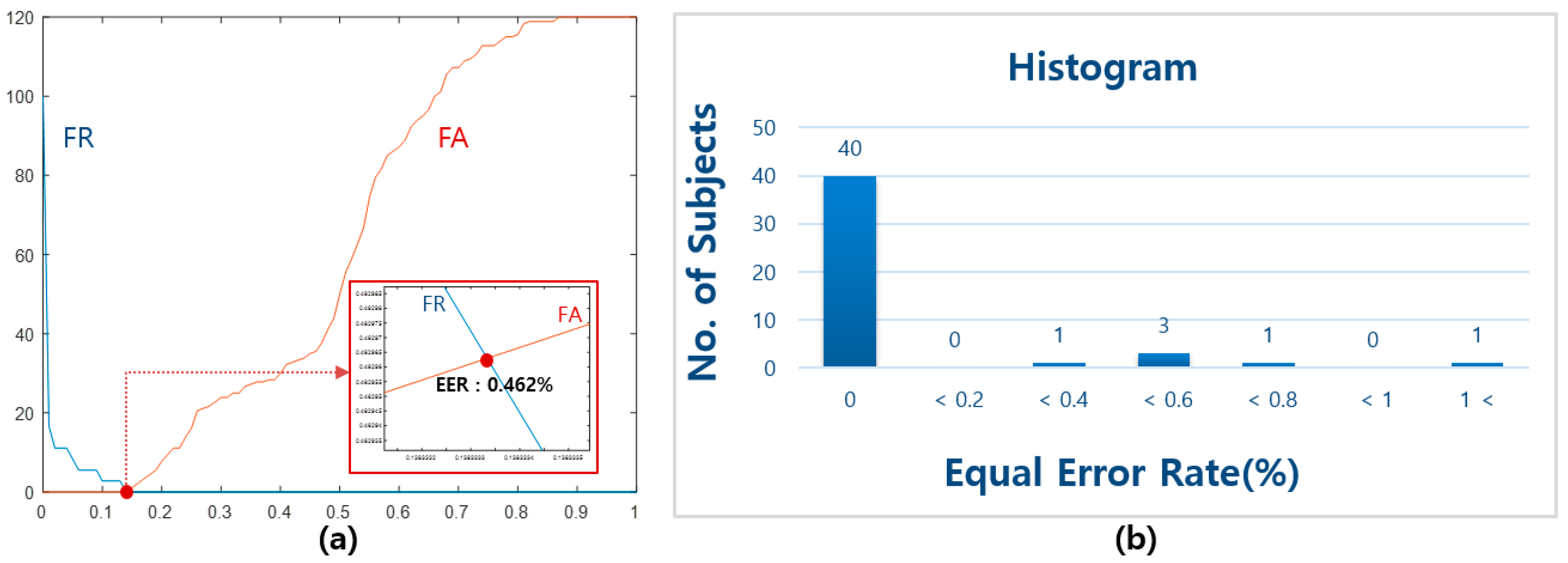
Figure 9a shows an example of obtaining the EER for each individual. A histogram of the EER (Equal Error Rates) is shown in Figure 9b. The average EER is 0.143%, which indicates the efficiency of the overall algorithm, as shown in Equation (32). Only a single user was enrolled at any point in time. In other words, at any point in time, we had one client and 46 imposters.

$$\mathrm{Total} \mathrm{efficiency} \mathrm{of} \mathrm{verification} = \frac{1}{\mathrm{No}. \mathrm{of} \mathrm{subject}}{\displaystyle {\displaystyle \sum }_{\mathrm{Sub}=1}^{\mathrm{No}. \mathrm{of} \mathrm{subject}}}{\mathrm{EER}}_{\mathrm{Sub}}$$

(32)

where Sub indicates the subject number.

To demonstrate the efficiency of our proposed algorithm, we compared it with related works that used the same database (MIT-BIH), as shown in

Table 1. Comparison of the proposed algorithm with related research using the same public database.

Ref.	NS	ST	DB	Method	EER	IDA
[48]	56	2-lead Direct Contact type	MITDB NSRDB PTB database	Normalized AC and LDA	3.8 %	96.2 %
[49]	145	2-lead Direct Contact type	(a) MITDB (b) NSRDB (c) LTSTDB	WT and ICA	(a) 0.43 % (b) 0.67 % (c) 1.89 %	(a) 99.57 % (b) 99.33 % (c) 98.11 %
[28]	50	2-lead Direct Contact type (Only single lead of data used)	MITDB NSRDB	Delineation of P and T wave, Correlation	1.01 %	98.99 %
[50]	73	2-lead Direct Contact type (Only single lead of data used)	(a) MITDB (b) IIT(BHU) database (laboratory experiment)	Delineation of P and T wave, Eigenbeat feature extraction	(a) 8.58 % (b) 4.45 %	(a) 91.42 % (b) 95.55 %
[51]	47	2-lead Direct Contact type (Only single lead of data used)	MITDB	Sum of Gaussian, QDA	3 %	97 %
[52]	83	2-lead Direct Contact type (Only single lead of data used), AliveCor single lead Contact type [54]	(a) MITDB NSRDB (b) Laboratory experiment database	FP (Time and amplitude), Proposed hierarchical algorithm	(a) 9.795 % (b) 8.18 %	(a) 90.205 % (b) 91.82 %
[53]	65	2-lead Direct Contact type (Only single lead of data used)	(a) MITDB (b) NSRDB	DWT	(a) 6.9 % (b) 0.6 %	(a) 93.1 % (b) 99.4 %
Proposed method	72	2-lead Direct Contact type (Only single lead of data used)	MITDB	Unnormalized AC and Interval based LDA algorithm	0.143 %	99.857 %

NS number of subject, ST sensor type, DB database, EER equal error rate, IDA identification accuracy, AC autocorrelation, LDA linear discriminant analysis, WT wavelet transform, ICA independent component analysis, QDA quadratic discriminant analysis, DWT discrete wavelet transform.

. Table 1 shows that the EER (Equal Error Rate) in Reference [48] is higher than the proposed algorithm despite using ECG data from two leads. Recently, most ECG wearable devices, such as smart watches, only use one lead; thus, the proposed algorithm is more suitable for real-life applications. In Reference [48], a fixed shifting size was used for the autocorrelation, while in the proposed algorithm, we used a flexible shifting size for the autocorrelation as the QRS width for the individual, which requires less computational effort. Although fused information from two ECG leads was used in Reference [49], their IDA (Identification Accuracy) is lower than the proposed algorithm; however, the enroll time is 5 min, which is longer than our algorithm. A fiducial point dependent method was used in References [28,50,51,52] which is vulnerable to noise. Only 10–20 s data were used for enrollment and verification in References [52,53]. However, we used two 2-min data for enrollment and verification to verify the stability of the proposed algorithm. Only a direct contact sensor was used in References [28,48,49,50,51,52,53] to verify the algorithms. In contrast, we used a non-contact single lead senor for real-life applications. In this paper, in the case of a fiducial dependent approach, although it has the advantage of being able to identify a subject in a relatively short time with less computational effort, it is easily affected by external noise. On the other hand, a fiducial independent approach has the advantage of being less affected by external noise, but it takes higher computational effort and longer authentication time. To compensate for the advantages and disadvantages of the above two methods, the amount of calculation was reduced through the amplitude feature using ACP and the identification accuracy was improved through the interval-based angle feature.

However, in this study, the matching score was calculated using the same weight for the two features, resulting in a disadvantage in terms of the weakness in various environmental variables. Therefore, we intend to explore the application of variable weights for future research to design a robust algorithm for environment variables.

4. Conclusions

In this paper, a novel interval-based LDA algorithm is proposed. The implementation experiments of the proposed algorithm show higher identification accuracy compared to the existing ECG-based identification algorithm using the fiducial point dependent method or fiducial independent method. Based on this algorithm, we can complement each method’s disadvantages by using both a fiducial point dependent method (amplitude distance by pixel) and fiducial point independent method (angle distance by feature vector). In addition, our proposed algorithm is able to maintain identification accuracy by tracking the ECG that changes in real-time using a template updating process.

This algorithm was tested with a public ECG database (MIT-BIH) and we compared its performance with related studies using the same database. The results show that the proposed algorithm is more reliable than other algorithms in terms of EER (Equal Error Rate). However, this algorithm has the disadvantage that it requires 5 s for each identification. Therefore, as future research, we intend to reduce the identification time and proceed to commercialize this as a product through multimodal identification combined with other biometrics.

References

1. Geddes, L.A.; Roeder, R.A. The first electronic electrocardiograph. Cardiovasc. Eng. Int. J. 2002, 2, 73–79. [Google Scholar] [CrossRef]
2. Myers, G.B.; Klein, H.A.; Stofer, B.E. The electrocardiographic diagnosis of right ventricular hypertrophy. Am. Heart J. 1948, 35, 1–40. [Google Scholar] [CrossRef]
3. Casale, P.N.; Devereux, R.B.; Alonso, D.R.; Campo, E.; Kligfield, P. Improved sex-specific criteria of left ventricular hypertrophy for clinical and computer interpretation of electrocardiograms: Validation with autopsy findings. Circulation 1987, 75, 565–572. [Google Scholar] [CrossRef] [PubMed] [Green Version]
4. Addison, P.S.; Watson, J.N.; Clegg, G.R.; Holzer, M.; Sterz, F.; Robertson, C.E. Evaluating arrhythmias in ECG signals using wavelet transforms. IEEE Eng. Med. Biol. Mag. 2000, 19, 104–109. [Google Scholar] [CrossRef] [PubMed]
5. Acharya, R.; Kannathal, N.; Krishnan, S.M. Comprehensive analysis of cardiac health using heart rate signals. Physiol. Meas. 2004, 25, 1139. [Google Scholar]
6. Bsoul, M.; Minn, H.; Tamil, L. Apnea MedAssist: Real-time Sleep Apnea Monitor Using Single-Lead ECG. IEEE Trans. Inf. Technol. Biomed. 2011, 15, 416–427. [Google Scholar] [CrossRef] [PubMed] [Green Version]
7. Karthikeyan, P.; Murugappan, M.; Yaacob, S. Detection of human stress using short-term ECG and HRV signals. J. Mech. Med. Biol. 2013, 13, 1350038. [Google Scholar] [CrossRef] [Green Version]
8. Kaniusas, E.; Pfutzner, H.; Mehnen, L.; Kosel, J.; Tellez-Blanco, C.; Varoneckas, G.; Alonderis, A.; Meydan, T.; Vazquez, M.; Rohn, M.; et al. Method for continuous nondisturbing monitoring of blood pressure by magnetoelastic skin curvature sensor and ECG. IEEE Sens. J. 2006, 6, 819–828. [Google Scholar] [CrossRef]
9. Saul, J.P.; Rea, R.F.; Eckberg, D.L.; Berger, R.D.; Cohen, R.J. Heart rate and muscle sympathetic nerve variability during reflex changes of autonomic activity. Am. J. Physiol. Circ. Physiol. 1990, 258, H713–H721. [Google Scholar] [CrossRef]
10. Pomeranz, B.; Macaulay, R.J.; Caudill, M.A.; Kutz, I.; Adam, D.; Gordon, D.; Kilborn, K.M.; Barger, A.C.; Shannon, D.C.; Cohen, R.J.; et al. Assessment of autonomic function in humans by heart rate spectral analysis. Am. J. Physiol. Circ. Physiol. 1985, 248, H151–H153. [Google Scholar] [CrossRef]
11. Agrafioti, F.; Gao, J.; Hatzinakos, D.; Yang, J. Heart biometrics: Theory, methods and applications. In Biometrics; InTech: Shanghai, China, 2011; pp. 199–216. [Google Scholar]
12. Biel, L.; Pettersson, O.; Philipson, L.; Wide, P. ECG analysis: A new approach in human identification. In Proceedings of the 16th IEEE Instrumentation and Measurement Technology Conference, Venice, Italy, 24–26 May 1999. [Google Scholar]
13. US Federal Trade Commission. Consumer Sentinel Network Data Book for January–December 2018. Available online: https://www.ftc.gov/system/files/documents/reports/consumer-sentinel-network-data-book-2018/consumer_sentinel_network_data_book_2018_0.pdf (accessed on 26 August 2020).
14. Burge, M.; Burger, W. Ear Biometrics. In Biometrics; Springer US: Boston, MA, USA, 1996; pp. 273–285. [Google Scholar]
15. Hossain, S.M.E.; Chetty, G. Next generation identity verification based on face-gait Biometrics. In Proceedings of the International Conference on Biomedical Engineering and Technology, Kuala Lumpur, Malaysia, 4–5 June 2011. [Google Scholar]
16. Prabhakar, S.; Pankanti, S.; Jain, A.K. Biometric recognition: Security and privacy concerns. IEEE Secur. Priv. 2003, 1, 33–42. [Google Scholar] [CrossRef]
17. Sanchit; Ramalho, M.; Correia, P.L.; Soares, L.D. Biometric identification through palm and dorsal hand vein patterns. In Proceedings of the 2011 IEEE EUROCON—International Conference on Computer as a Tool, Lisbon, Portugal, 27–29 April 2011; pp. 1–4. [Google Scholar]
18. Boulgouris, N.V.; Plataniotis, K.N.; Micheli-Tzanakou, E. (Eds.) Biometrics: Theory, Methods, and Applications; John Wiley & Sons, Inc.: Hoboken, NJ, USA, 2009; Volume 9, ISBN 9780470522356. [Google Scholar]
19. Jain, A.K.; Arun, R.; Salil, P. An introduction to biometric recognition. IEEE Trans. Circuits Syst. Video Technol. 2004, 14, 4–20. [Google Scholar] [CrossRef] [Green Version]
20. Israel, S.A.; Irvine, J.M.; Cheng, A.; Wiederhold, M.D.; Wiederhold, B.K. ECG to identify individuals. Pattern Recognit. 2005, 38, 133–142. [Google Scholar] [CrossRef]
21. Irvine, J.; Israel, S.; Wiederhold, M.; Wiederhold, B. A new biometric: Human identification from circulatory function. In Proceedings of the Joint Statistical Meetings of the American Statistical Association, San Francisco, CA, USA, 3–7 August 2003. [Google Scholar]
22. Zhang, Z.; Wei, D. A New ECG Identification Method Using Bayes’ Teorem. In Proceedings of the Tencon 2006 IEEE Region 10 Conference, Hong Kong, China, 14–17 November 2006. [Google Scholar]
23. Singh, Y.N.; Gupta, P. ECG to Individual Identification. In Proceedings of the 2008 IEEE Second International Conference on Biometrics: Theory, Applications and Systems, Arlington, VA, USA, 29 September–1 October 2008. [Google Scholar]
24. Simon, B.P.; Eswaran, C. An ECG Classifier Designed Using Modified Decision Based Neural Networks. Comput. Biomed. Res. 1997, 30, 257–272. [Google Scholar] [CrossRef] [PubMed]
25. Hoekema, R.; Uijen, G.J.H.; van Oosterom, A. Geometrical aspects of the interindividual variability of multilead ECG recordings. IEEE Trans. Biomed. Eng. 2001, 48, 551–559. [Google Scholar] [CrossRef] [PubMed]
26. Tan, R.; Perkowski, M. ECG Biometric Identification Using Wavelet Analysis Coupled with Probabilistic Random Forest. In Proceedings of the 2016 15th IEEE International Conference on Machine Learning and Applications (ICMLA), Anaheim, CA, USA, 18–20 December 2016. [Google Scholar]
27. Agrafioti, F.; Hatzinakos, D.; Bui, F.M. Cardiac biometric security in welfare monitoring. In Proceedings of the 2012 IEEE International Conference on Acoustics, Speech and Signal Processing (ICASSP), Kyoto, Japan, 25–30 March 2012. [Google Scholar]
28. Singh, Y.N.; Gupta, P. Correlation-based classification of heartbeats for individual identification. Soft Comput. 2011, 15, 449–460. [Google Scholar] [CrossRef]
29. Fratini, A.; Sansone, M.; Bifulco, P.; Cesarelli, M. Individual identification via electrocardiogram analysis. Biomed. Eng. Online 2015, 14, 78. [Google Scholar] [CrossRef] [Green Version]
30. Singh, Y.N.; Singh, S.K. Evaluation of Electrocardiogram for Biometric Authentication. J. Inf. Secur. 2011, 03, 39–48. [Google Scholar] [CrossRef] [Green Version]
31. Guennoun, M.; Abbad, N.; Talom, J.; Rahman, S.M.M.; El-Khatib, K. Continuous authentication by electrocardiogram data. In Proceedings of the 2009 IEEE Toronto International Conference Science and Technology for Humanity (TIC-STH), Toronto, ON, Canada, 26–27 September 2009. [Google Scholar]
32. Kyoso, M.; Uchiyama, A. Development of an ECG identification system. In Proceedings of the 2001 Conference Proceedings of the 23rd Annual International Conference of the IEEE Engineering in Medicine and Biology Society, Istanbul, Turkey, 25–28 October 2001. [Google Scholar]
33. Kass, R.E.; Colleen, E.C. (Eds.) Basis and Treatment of Cardiac Arrhythmias; Springer Science & Business Media: Berlin/Heidelberg, Germany, 2005; Volume 171. [Google Scholar]
34. Physionet, Physiobank Archives, Massachusetts Institute of Technology Cambridge, January 2011. Available online: https://www.physionet.org/physiobank/database/#ecg (accessed on 26 August 2020).
35. Sörnmo, L.; Laguna, P. Bioelectrical Signal Processing in Cardiac and Neurological Applications; Academic Press: New York, NY, USA, 2005; Volume 8. [Google Scholar]
36. Chan, A.D.C.; Hamdy, M.M.; Badre, A.; Badee, V. Wavelet Distance Measure for Person Identification Using Electrocardiograms. IEEE Trans. Instrum. Meas. 2008, 57, 248–253. [Google Scholar] [CrossRef]
37. Ye, C.; Coimbra, M.T.; Vijaya Kumar, B.V.K. Arrhythmia detection and classification using morphological and dynamic features of ECG signals. In Proceedings of the 2010 Annual International Conference of the IEEE Engineering in Medicine and Biology, Buenos Aires, Argentina, 31 August–4 September 2010. [Google Scholar]
38. Belgacem, N. ECG Based Human Authentication using Wavelets and Random Forests. Int. J. Cryptogr. Inf. Secur. 2012, 2, 1–11. [Google Scholar] [CrossRef]
39. Choudhary, T.; Manikandan, M.S. A novel unified framework for noise-robust ECG-based biometric authentication. In Proceedings of the 2015 2nd International Conference on Signal Processing and Integrated Networks (SPIN), Noida, India, 19–20 February 2015. [Google Scholar]
40. Gutta, S. Biomedical Signal Processing and Inference in Wearable Sensing Applications. Ph.D. Thesis, Oklahoma State University, Stillwater, OK, USA, 1 December 2016. [Google Scholar]
41. Plataniotis, K.N.; Hatzinakos, D.; Lee, J.K.M. ECG Biometric Recognition Without Fiducial Detection. In Proceedings of the 2006 Biometrics Symposium: Special Session on Research at the Biometric Consortium Conference, Baltimore, MD, USA, 19–21 September 2006. [Google Scholar]
42. Matta, R.; Lau, J.K.H.; Agrafioti, F.; Hatzinakos, D. Real-Time Continuous Identification System Using ECG Signals. In Proceedings of the 2011 Canadian Conference on Electrical and Computer Engineering, Niagara Falls, ON, Canada, 8–11 May 2011; pp. 1313–1316. [Google Scholar]
43. Wang, Y.; Agrafioti, F.; Hatzinakos, D.; Plataniotis, K.N. Analysis of Human Electrocardiogram for Biometric Recognition. EURASIP J. Adv. Signal Process. 2007, 2008, 148658. [Google Scholar] [CrossRef] [Green Version]
44. Safie, S.I.; Soraghan, J.J.; Petropoulakis, L. Pulse Active Ratio (PAR): A new feature extraction technique for ECG biometric authentication. In Proceedings of the 2011 IEEE International Conference on Signal and Image Processing Applications (ICSIPA), Kuala Lumpur, Malaysia, 16–18 November 2011. [Google Scholar]
45. Mücke, D. Elektrokardiographie Systematisch; UNI-MED-Verlag: Bremen, Germany, 1996. [Google Scholar]
46. Khalil, I.; Sufi, F. Legendre Polynomials based biometric authentication using QRS complex of ECG. In Proceedings of the 2008 International Conference on Intelligent Sensors, Sensor Networks and Information Processing, Sydney, Australia, 15–18 December 2008. [Google Scholar]
47. Pan, J.; Tompkins, W.J. A Real-Time QRS Detection Algorithm. IEEE Trans. Biomed. Eng. 1985, BME-32, 230–236. [Google Scholar] [CrossRef] [PubMed]
48. Agrafioti, F.; Hatzinakos, D. ECG biometric analysis in cardiac irregularity conditions. Signal, Image Video Process. 2009, 3, 329–343. [Google Scholar] [CrossRef]
49. Ye, C.; Coimbra, M.T.; Kumar, B.V.K.V. Investigation of human identification using two-lead Electrocardiogram (ECG) signals. In Proceedings of the 2010 Fourth IEEE International Conference on Biometrics: Theory, Applications and Systems (BTAS), Washington, DC, USA, 27–29 September 2010. [Google Scholar]
50. Singh, Y.N.; Singh, S.K. Identifying Individuals Using Eigenbeat Features of Electrocardiogram. J. Eng. 2013, 2013, 539284. [Google Scholar] [CrossRef] [Green Version]
51. Sarkar, A.; Abbott, A.L.; Doerzaph, Z. ECG biometric authentication using a dynamical model. In Proceedings of the 2015 IEEE 7th International Conference on Biometrics Theory, Applications and Systems (BTAS), Arlington, VA, USA, 8–11 September 2015. [Google Scholar]
52. Arteaga-Falconi, J.S.; Al Osman, H.; El Saddik, A. ECG Authentication for Mobile Devices. IEEE Trans. Instrum. Meas. 2016, 65, 591–600. [Google Scholar] [CrossRef]
53. Dar, M.N.; Akram, M.U.; Usman, A.; Khan, S.A. ECG biometric identification for general population using multiresolution analysis of DWT based features. In Proceedings of the 2015 Second International Conference on Information Security and Cyber Forensics (InfoSec), Cape Town, South Africa, 15–17 November 2015. [Google Scholar]
54. Heart Monitor AC-002 User Manual; AliveCor, Inc.: San Francisco, CA, USA, 2015.
Figure 1. Basic ECG signal cycle.
Applsci 10 06025 g001
Figure 2. Simplified block diagram of the proposed interval-based LDA algorithm.
Applsci 10 06025 g002
Figure 3. ECG signal preprocessing. (a): The simplified block diagram of signal preprocessing, where the BPF and notch filter are applied to remove the noise and power line interference related harmonics on ECG signals. (b): An example of an ECG signal before and after the preprocessing.
Applsci 10 06025 g003
Figure 4. The two-minute-long training set x ( n ) and its time-shifted version x ( n + m ) . The training set x ( n ) is divided into C classes, each of which is N samples long. For example, x 1 ( n ) and x 1 ( n + m ) are the 1st class of x ( n ) and x ( n + m ) , respectively.
Applsci 10 06025 g004
Figure 5. An example of a set of ACPs, displayed together within the same time period of Q, for two different subjects (subject A and subject B) when C = 5. (ad) illustrate the differences in amplitude and angle patterns of ACPlet generated when the ACPs are segmented into six ACPlets, even though the two subjects have a very similar ACP shape.
Applsci 10 06025 g005
Figure 6. Symbol descriptions: (a) N is the update cycle of the verification process; (b) Q is the time-shifting size of the ACP process; (c) L is the size of an interval and the maximum length that satisfies the MSE (ζ) criterion.
Applsci 10 06025 g006
Figure 7. The relationship between the MSE (Mean Squared Error) ζ and the IDA (Identification Accuracy) η according to NI (Number of Interval) values to show the decision of the optimal NI. In this experiment, the optimal NI is set as the value when η     = 99.646% and ζ = ε
Applsci 10 06025 g007
Figure 8. Examples of false rejection and acceptance rates for Subject no. 1, no. 2, and no. 3.
Applsci 10 06025 g008
Figure 9. (a) Example of the EER depending on individuals (subject no. 41); (b) a histogram of the EER (Equal Error Rates) (average EER is 0.143%).
Applsci 10 06025 g009