Article

A Comparison of Human against Machine-Classification of Spatial Audio Scenes in Binaural Recordings of Music

1
Faculty of Computer Science, Białystok University of Technology, 15-351 Białystok, Poland
2
Applied Psychoacoustics Laboratory (APL), University of Huddersfield, Huddersfield HD1 3DH, UK
*
Author to whom correspondence should be addressed.
Appl. Sci. 2020, 10(17), 5956; https://doi.org/10.3390/app10175956
Submission received: 30 July 2020 / Revised: 21 August 2020 / Accepted: 25 August 2020 / Published: 28 August 2020

Abstract

:
The purpose of this paper is to compare the performance of human listeners against the selected machine learning algorithms in the task of the classification of spatial audio scenes in binaural recordings of music under practical conditions. The three scenes were subject to classification: (1) music ensemble (a group of musical sources) located in the front, (2) music ensemble located at the back, and (3) music ensemble distributed around a listener. In the listening test, undertaken remotely over the Internet, human listeners reached the classification accuracy of 42.5%. For the listeners who passed the post-screening test, the accuracy was greater, approaching 60%. The above classification task was also undertaken automatically using four machine learning algorithms: convolutional neural network, support vector machines, extreme gradient boosting framework, and logistic regression. The machine learning algorithms substantially outperformed human listeners, with the classification accuracy reaching 84%, when tested under the binaural-room-impulse-response (BRIR) matched conditions. However, when the algorithms were tested under the BRIR mismatched scenario, the accuracy obtained by the algorithms was comparable to that exhibited by the listeners who passed the post-screening test, implying that the machine learning algorithms capability to perform in unknown electro-acoustic conditions needs to be further improved.

1. Introduction

Following its success in virtual-reality applications [1,2,3], binaural technology is now being gradually adopted by professional and amateur broadcasters [4,5], with a prospect of becoming a prominent “tool” for delivering 3D audio content over the Internet. Binaural technology was recently introduced to one of the most popular video sharing services [6]. Consequently, one may expect that large repositories of spatial audio recordings, stored in a binaural format, will be created soon. This will inevitably give rise to new challenges related to the search and retrieval of “spatial audio information” from such recordings.
There are several reasons for which the research into the automatic spatial audio scene classification in binaural recordings is important. The outcomes of such research could help to design systems for the semantic search and retrieval of audio content in binaural recordings based on spatial information, allowing listeners to explore Internet resources looking for recordings (or their selected excerpts) with a music ensemble located at particular directions, e.g., behind the head of a listener. Moreover, the algorithm for the automatic spatial audio scene classification can be used as a building block of spatial audio quality prediction systems (the performance of spatial quality prediction systems can be improved by providing them with information on spatial audio scene characteristics [7]). Additionally, in the authors’ opinion, the automatic spatial scene classifiers could facilitate the operation of the audio format conversion algorithms used for the up-mixing of binaural signals to multichannel loudspeaker signals. Furthermore, they might be exploited as an automatic preselection tool for gathering audio material for subjective audio quality assessment tests. While the application context in this paper is limited to the domain of reproduced audio, the algorithms for the automatic spatial scene recognition could also be embedded in environment-aware binaural hearing aids, adapting their parameters depending on the surrounding audio scenes.
Most of the research within the area of machine listening of binaural audio recordings has been focused on the localization of individual audio sources [8,9], ignoring higher-level descriptors of complex spatial audio scenes. This study belongs to an emerging field of research aiming to develop the machine learning methods for the holistic characterization of spatial audio scenes for reproduced sound [10,11]. It builds on our previous work on the automatic spatial audio scene classification of the binaural recordings using traditional machine learning methods [12,13] and on our recent pilot study employing a deep learning approach [14].
The aim of this work is to compare the performance of human listeners against the performance of the modern machine learning algorithms in the task of the classification of the basic spatial audio scenes in synthetically generated but practical binaural recordings of music. The rationale for undertaking this topic comes from the observation that with the advent of modern machine learning algorithms, most notably deep learning techniques, for some classifications tasks, such as image recognition, the performance level of the computational algorithms matched or even exceeded that exhibited by humans [15]. Therefore, it was interesting to find out how this human–machine comparison would turn out in the case of this new field of research.
The following three scenes were considered in the study: (1) music ensemble (a group of musical sound sources) located in the front of a listener, (2) music ensemble located at the back of a listener, and (3) music ensemble distributed around a listener in the horizontal plane (scenes encompassing a height dimension were left for future work).
In this study, 212 listeners were recruited to classify the binaural audio excerpts according to the aforementioned three spatial scenes. The listening test was undertaken internationally over the Internet in realistic or semi-realistic conditions; that is, in an environment typical for ordinary listeners listening to binaural music recordings using headphones (with uncontrolled electro-acoustic conditions). Head-tracking systems and the technique of individualization of head-related transfer functions (HRTFs) were not used in this study as most of the ordinary listeners of binaural audio content still do not exploit such facilities.
Each listener was requested to classify 30 binaural music excerpts, randomly drawn from the repository of 1560 recordings. In total, 1560 binaural excerpts were classified by the listeners. The same task was also undertaken automatically, exploiting four machine learning algorithms—convolutional neural network (CNN), support vector machines (SVM), extreme gradient boosting framework (XGBoost), and logistic regression (Logit)—allowing for a comparison of the classification accuracy reached by the human listeners with those obtained using the machine audition algorithms. To the best of the authors’ knowledge, this is the first study aiming to undertake such a comparison.
The paper is organized as follows. The next section provides the background of this study. Section 3 describes the corpus of the binaural music recordings used both in the listening test and in the experiments with the automatic classification of spatial audio scenes. Section 4 and Section 5 elaborate on the methodology and the results obtained using the listeners and the machine learning algorithms, respectively. The outcome of the comparison and the drawn conclusions are discussed and summarized in the final two sections.

2. Background

2.1. Binaural Perception by Humans and Machines

For humans and machines alike, spatial perception of audio sources in the horizontal plane is facilitated by such binaural cues as interaural time difference (ITD), interaural level difference (ILD), and interaural coherence (IC) [2]. In addition, spectral cues help to localize audio sources in the median plane [16]. Since real-world binaural recordings of music typically contain a large number of spatially distributed and simultaneously sound-emitting sources, the above cues get confounded, particularly under reverberant conditions. Hence, the automatic classification of complex audio scenes in binaural recordings of music is not a trivial task.
An important limitation of binaural listening (both in humans and machines), resulting in localization errors between front and back hemispheres, is caused by the ambiguity of binaural cues—a mechanism referred to as a cone-of-confusion effect [17]. To reduce the influence of the above effect, humans exploit involuntary micro head movements [18].

2.2. The State-of-the-Art Models

While the initial models mimicking binaural hearing in humans allowed for the localization of only single sources under anechoic conditions [19,20], the state-of-the-art algorithms are capable of localizing several sources simultaneously, both in anechoic and reverberant environments [9,21,22,23,24]. While some of the advanced models still employ a form of feature extraction combined with traditional classification algorithms such as Gaussian mixture models [21], the algorithms developed more recently commonly utilize deep learning techniques [22,23,24,25]. Binaural signals can be either used directly at the input of the deep neural networks [26] or indirectly through some forms of signal preprocessing. Such preprocessing may involve a traditional feature extraction [21], calculation of the cross-correlation function from the left and right channel signals [22,23,24,25], or converting sounds into “images” in the form of spectrograms [27]. The first and the last approaches were also adopted in this study.
While the state-of-the-art algorithms allow for the accurate localization of simultaneously sound-emitting audio sources in binaural signals, they have major drawbacks, preventing them from being directly applicable to the automatic classification of scenes in the binaural recordings of music. Firstly, these algorithms typically require an a priori knowledge on the “number” and “characteristics” of the individual sources in an analyzed scene [21,22,23,24]. Such information is normally unavailable for real-life music recordings reposited in the Internet. Secondly, to reduce the rate of front–back localization errors, some algorithms include mechanisms mimicking the head movements. While such algorithms can be applied to the systems equipped with robotic dummy-head microphones [28] or to the systems involving adaptive synthesis of binaural signals [23], they cannot be applied to the recordings obtained with a static head methodology (a scenario pertinent to this study). Finally, the above algorithms were developed and tested using either speech or contrived noise signals. Since they were not intended for audio (music) signals, it is unknown whether they could be “transferred” and applied to music signals.

2.3. Related Work

There are many reports in the literature concerning either “computational auditory scene analysis” (CASA) [29] or “acoustic scene classification” (ASC) [30,31]. The aim of CASA is to isolate individual audio objects within a complex scene, whereas the purpose of ASC is to identify an acoustic environment wherein a given auditory event took place. Therefore, despite their nomenclature similarity, such studies are fundamentally different compared to the work presented in this paper, which is focused on the classification of the spatial audio scenes.
Woodcock et al. [32] recently published a study investigating the subjective classification of complex auditory scenes in spatial audio recordings reproduced using a multichannel loudspeaker system. In contrast to this work, their research aim was to characterize audio objects “inside” sound scenes (within-scene categorization) rather than to perform a differentiation between scenes (between-scene classification).
The purpose of many listening tests involving binaural hearing, reported in the literature, has often been limited to the localization of individual audio sources [8,16,18,22]. They are normally undertaken under highly controlled laboratory conditions. To maintain the ecological validity of the experiments, in this study the listening tests were carried out under more realistic conditions, similar to those encountered by typical listeners while auditioning audio recordings from the Internet. To the best of the authors’ knowledge, no large-scale listening test (involving a large group of listeners) has been conducted regarding the perception of spatial scenes exhibited by binaural recordings under ecologically valid conditions.

3. Repository of Binaural Audio Recordings

In this work, we used the same collection of binaural audio excerpts as in our previous study [13]. To the best of the authors’ knowledge, this is currently the only audio repository intended for research into human or machine perception of spatial audio scenes in binaural recordings available in the public domain.
The repository consists of the two sets of the audio excerpts intended for the development of machine learning algorithms (training) and their evaluation (testing), respectively. To create this repository, initially, 152 multi-track studio recordings were gathered, out of which 112 were allocated for training, whereas the remaining 40 items were destined for testing, as shown in Table 1. These multi-track recordings represented a broad range of music genres, including classical music orchestral excerpts, opera, pop music, jazz, country, electronica, dance, rock, and heavy metal. The number of individual foreground audio objects (musical instruments or singers) in the group of recordings intended for training ranged from 5 to 62, with a median of 9. In the case of the recordings selected for testing, the number of foreground objects varied from 5 to 42, with a median being equal to 10.
The binaural excerpts were synthesized by convolving the abovementioned multi-track studio recordings with 13 sets of binaural-room-impulse-responses (BRIRs). Each multitrack recording was convolved in three variants, forming the following three spatial scenes:
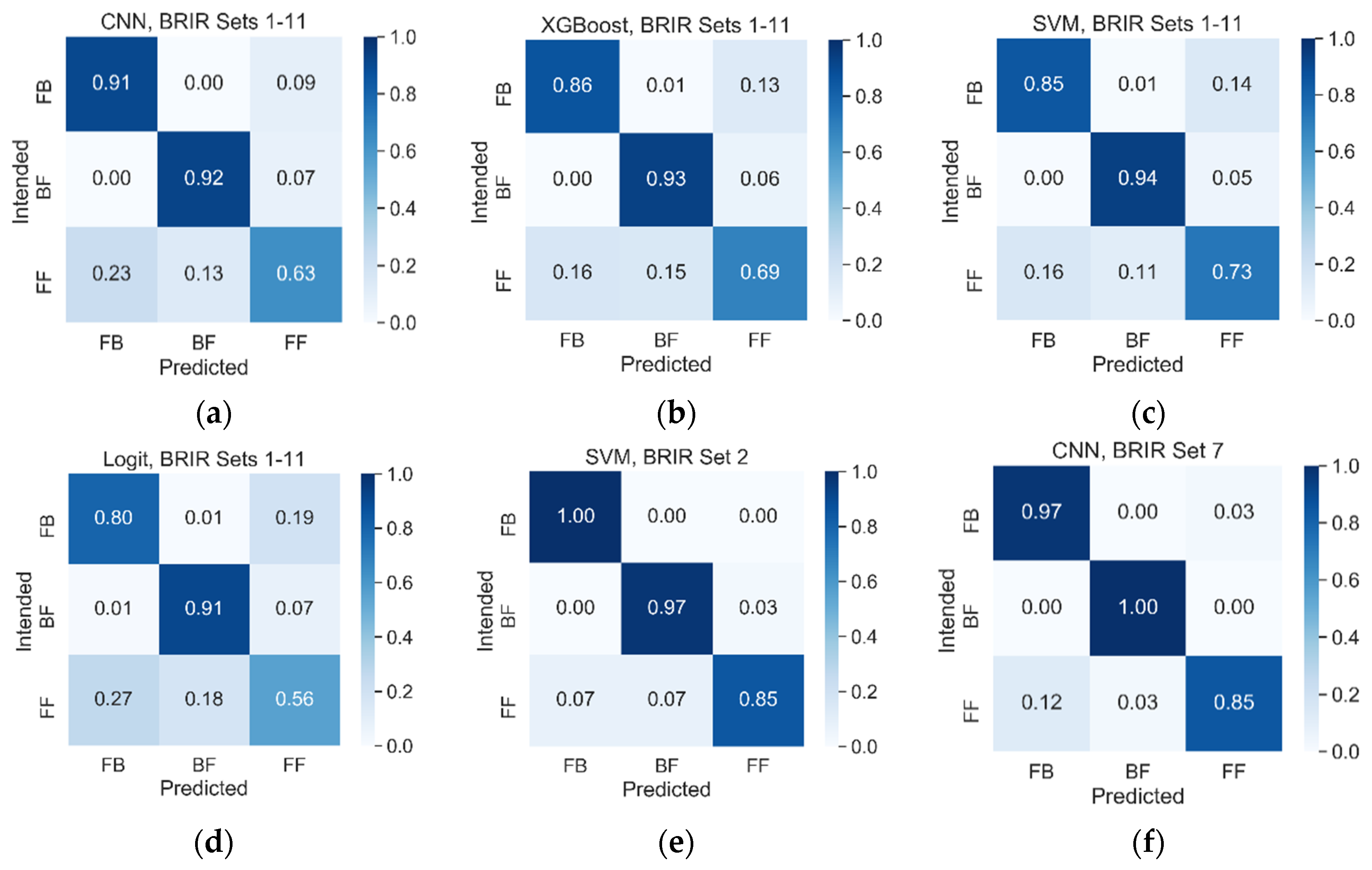
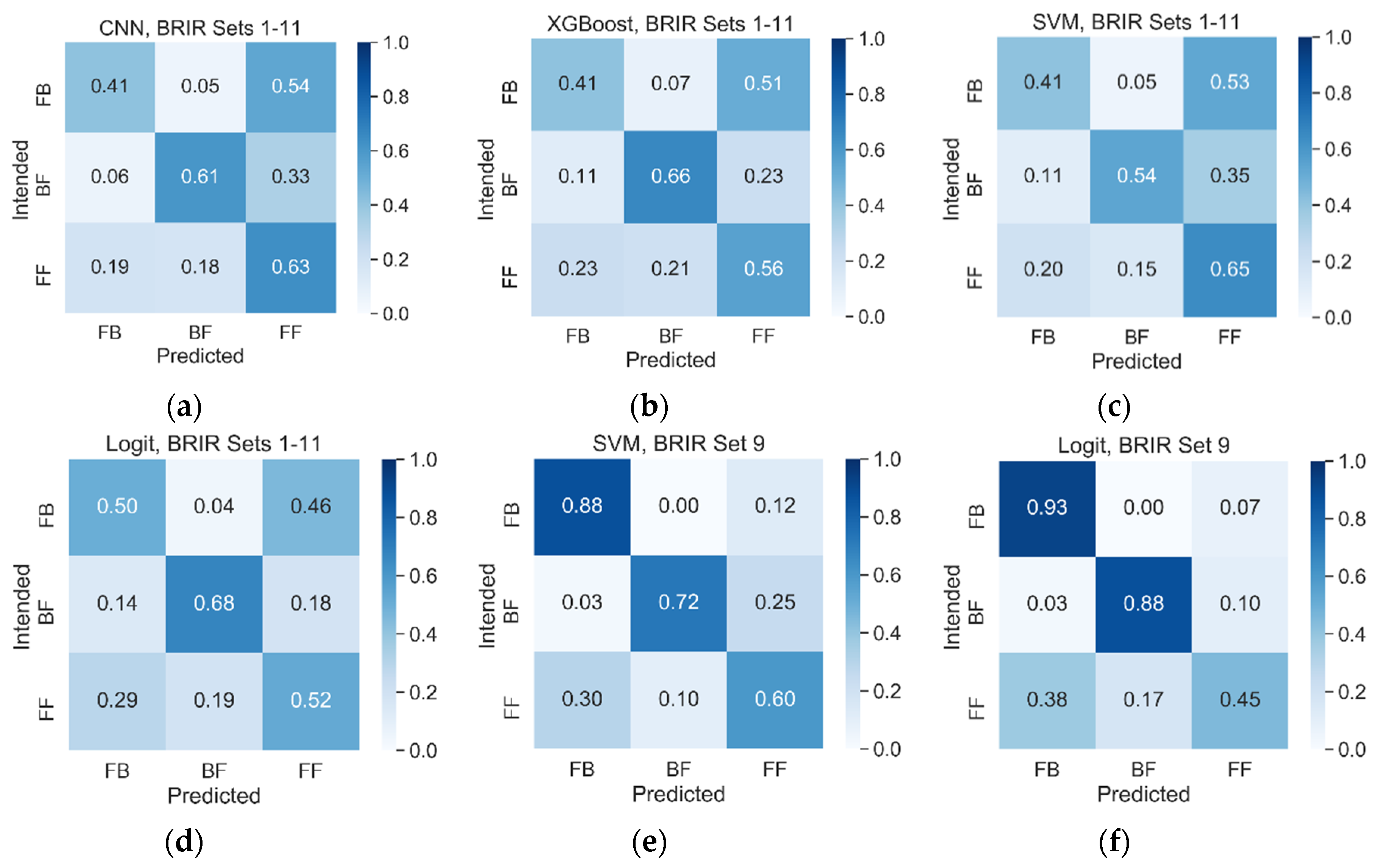
  • Foreground–Background (FB) scene—foreground content (music ensemble) located in front of a listener and background content, such as reverberations and room reflections, arriving from the back of a listener. This is a conventional “stage-audience” scenario [33], often used in jazz and classical music recordings.
  • Background–Foreground (BF) scene—background content in front of a listener with foreground content perceived from the back (a reversed stage-audio scenario). While it is infrequently used in music recordings, it was included in this study for completeness, as a symmetrically “flipped” counterpart of the previous scene.
  • Foreground–Foreground (FF) scene—foreground content both in front of and behind a listener, surrounding a listener in a horizontal plane. This scene is often used in binaural music recordings, e.g., in electronica, dance, and pop music (360° source scenario [33]).
While the number of the aforementioned scenes may initially appear to be small, it has to be emphasized that these three scenes are considerably challenging to identify aurally, in particular, when head-movements and individualized head-related-transfer-functions (HRTFs) are not incorporated in a binaural playback system. Head-tracking facilities and the technique of individualization of HRTFs were deliberately excluded from this work to maintain the ecological validity of the experiments as most of the ordinary listeners of binaural audio content do not use head tracking or individual HRTFs.
In total, 4368 excerpts were synthesized for training purposes (112 raw recordings × 13 sets of BRIRs × 3 scenes) and 1560 excerpts were synthesized for testing (40 raw recordings × 13 sets of BRIRs × 3 scenes), as indicated in Table 1. While the BRIR sets were the same for the training and testing repositories, the studio multi-track recordings were different for both collections. Hence, there were no common music recordings shared across the two repositories.
The BRIR sets used to synthesize the binaural excerpts were captured in venues representing both semi-anechoic and reverberant acoustic conditions, with reverberation time ranging from 0.17 to 2.1 s. The BRIR sets were recorded using three types of dummy-head microphones. They were all acquired from publicly available repositories (see Table 2 for an overview).
The duration of each excerpt was truncated to 7 s. The convolved recordings were stored in uncompressed two-channel stereo “wav” files, sampled at a rate of 48 kHz with a 24 bit resolution. The synthesized excerpts were labelled as FB, BF, and FF, respectively, depending on their spatial scenes. To avoid data compression effects, in the developed web application (described in the next section), the audio excerpts were not streamed but delivered to the listeners as uncompressed audio files. The above procedure of the synthesis of the binaural excerpts was only outlined here, with a detailed description provided in our former paper [13]. For the research reproducibility, the repository was made publicly available in Zenodo [34].

4. Human-Performed Classification

4.1. Stimuli

For consistency of comparison between human listeners and machine learning algorithms, the same group of 1560 binaural audio excerpts, intended for testing (see Table 1), was employed both in the listening test and in the evaluation of the aforementioned algorithms (the excerpts are available in Zenodo [34]). It would be too time-consuming for the participants to listen to all the excerpts. Therefore, each listener was asked to classify only 30 audio items, randomly drawn from the above group. To avoid confusing listeners with the recordings exhibiting different reverberation time, the excerpts synthesized with the same BRIR set were selected for a given listener. It was assumed by the authors that this could also help participants to accommodate to a given room’s acoustics.

4.2. Listeners

Due to a large number of listeners needed to collectively classify 1560 binaural audio excerpts, it would be impractical to recruit only critical listeners (participants possessing skills and experience in critical listening to spatial audio). Therefore, the invitation to partake in the experiment was open to both experienced and naïve listeners, as described in detail below.
Out of 212 listeners who took part in the test, 72 participants were recruited from the student population enrolled for the undergraduate and postgraduate courses in computer science at Białystok University of Technology. They carried out their tests on site in typical computer labs. The remaining 140 participants performed the tests remotely, over the Internet. They were recruited via social media, e.g., through the groups gathering binaural audio professionals and enthusiasts, as well as using email requests sent to the students of audio-related courses at several universities in Poland and the UK. Based on their IP addresses, 179 participants were from Poland, whereas the remaining listeners performed the tests in Germany, the UK, the USA, Switzerland, Japan, Italy, Netherlands, Austria, South Africa, France, Ireland, Belarus, and Belgium.
Most of the listeners (70%) could be characterized as naïve. A group of 64 subjects (30%) declared that they had formerly taken part in listening tests, although the nature of their listening experience is unknown (it is uncertain whether the former tests considered timbral or spatial aspects of audio reproduction). Five listeners (2%) self-declared hearing difficulties. No further information regarding the nature of these difficulties was acquired. Since according to Blauert [17], perception of spatial audio is relatively unaffected by typical hearing losses (e.g., age-related), provided that they are symmetric in both ears, it was decided to retain the data from these listeners.

4.3. Acoustical Conditions

A panel of 72 listeners undertook the tests in the typical computer laboratories (untreated acoustically), using closed-back Sennheiser HD 215 headphones and Lexicon Alpha audio interface. Background noise was not measured. The listeners were requested to adjust the playback volume according to their personal preferences. The remaining 136 listeners carried out their listening tests in unknown and uncontrolled environments. However, they were requested to report the manufacturer and the model of the headphones used. From the responses obtained, the listeners used a variety of headphones, ranging from consumer-level headsets to professional ones. The examples of 79 models of the headphones, as reported by the listeners, are listed in Appendix A. Some models of the headphones employed an active noise reduction system, potentially degrading the faithfulness of a spatial audio reproduction.
Due to a large variety of the headphones used in the listening tests and likely large variations in acoustical environments, the experimental conditions could be considered as representative of real-life binaural listening scenarios. To further maintain the ecological validity of the test:
  • a mechanism supporting head movements was not incorporated in the playback system (no head-tracking devices used),
  • no headphones frequency-response compensation was applied,
  • no individualized HRTFs were incorporated.

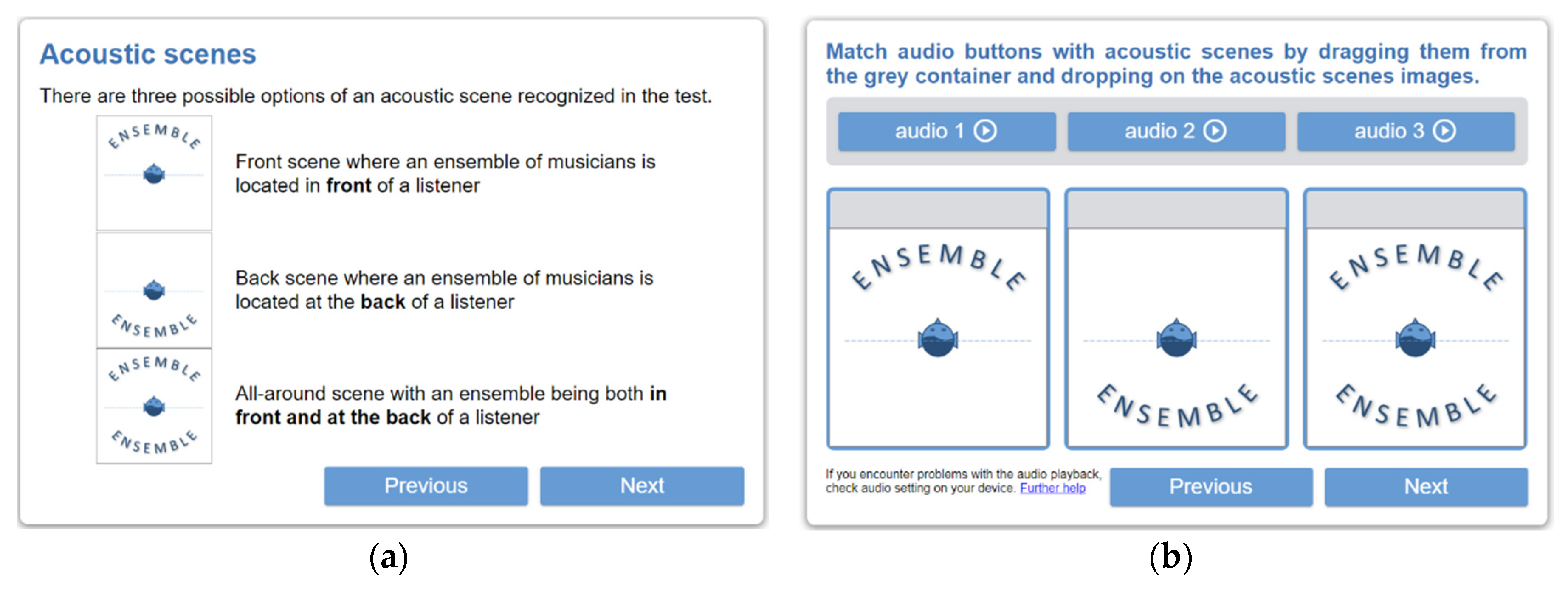
4.4. Classification Method

The participants were requested to classify each stimulus as representing one of the three spatial scenes. Initially, a single-stimulus paradigm was followed whereby the listeners were exposed to only one audio excerpt at a time. However, according to the pilot results, omitted in the paper due to space limitations, the test proved to be too challenging, yielding the results close to statistical “noise.” Therefore, in the improved version of the test, reported below, a triple-stimulus paradigm was adopted. The reason for such modification was motivated by the well-known phenomenon that humans have a weak discrimination ability when they are asked to characterize a single auditory stimulus at a time, but they are very acute at hearing differences between stimuli if they have an opportunity to make side-by-side auditory comparisons [41]. Therefore, in each trial of the test, the listeners had access to three stimuli, representing the three spatial scenes of a given multitrack recording. To facilitate the test, a custom-designed web-application was developed. Figure 1 illustrates its graphical user interface.
Prior to the commencement of the listening test, the participants were informed about its purpose, terms, and privacy policy. All subjects gave their informed consent for inclusion before they participated in the study. Then, they were requested to provide information about their previous listening test experience (if any), hearing difficulties, and the model of the headphones used. The data were collated anonymously.
In the next phase, the listeners were provided with a tutorial, graphically explaining the differences between the three basic spatial audio scenes (see Figure 1a). Subsequently, they were requested to undertake a guided equipment check, in order to verify the playback system and adjust its volume. This procedure also included the left and right channel checks.
During the listening test, the subjects were sequentially presented with triplets of stimuli, which could be auditioned by pressing one of the three buttons, labeled as “audio 1”, “audio 2”, and “audio 3”, respectively, as illustrated in Figure 1b. These stimuli represented the three spatial scenes (FB, BF, and FF) of a given multitrack recording (e.g., a jazz recording). The items could be auditioned in any order and switched at any time, at the discretion of a listener. The switching was undertaken synchronously, with a 10 ms cross-fade (with a raised cosine function) to avoid sound distortions. The task given to the listeners was to “match audio buttons with acoustic scenes by dragging them from the grey container and dropping on the acoustic scenes images”, as shown in Figure 1b.
The test consisted of 10 trials. Consequently, each listener was asked to classify 30 items in total (10 trails × 3 items), randomly drawn from the repository of 1560 excerpts. Since 212 subjects took part in the test, each excerpt was classified at least four times (1440 items were classified four times, whereas the remaining 120 excerpts were classified five times). There were no time limits imposed on the participants. The mean duration of the listening test was equal to approximately 8 min.
The experimental protocol employed in the listening test was approved by the Ethics Committee of the Białystok University of Technology (Project Code 2/2020).

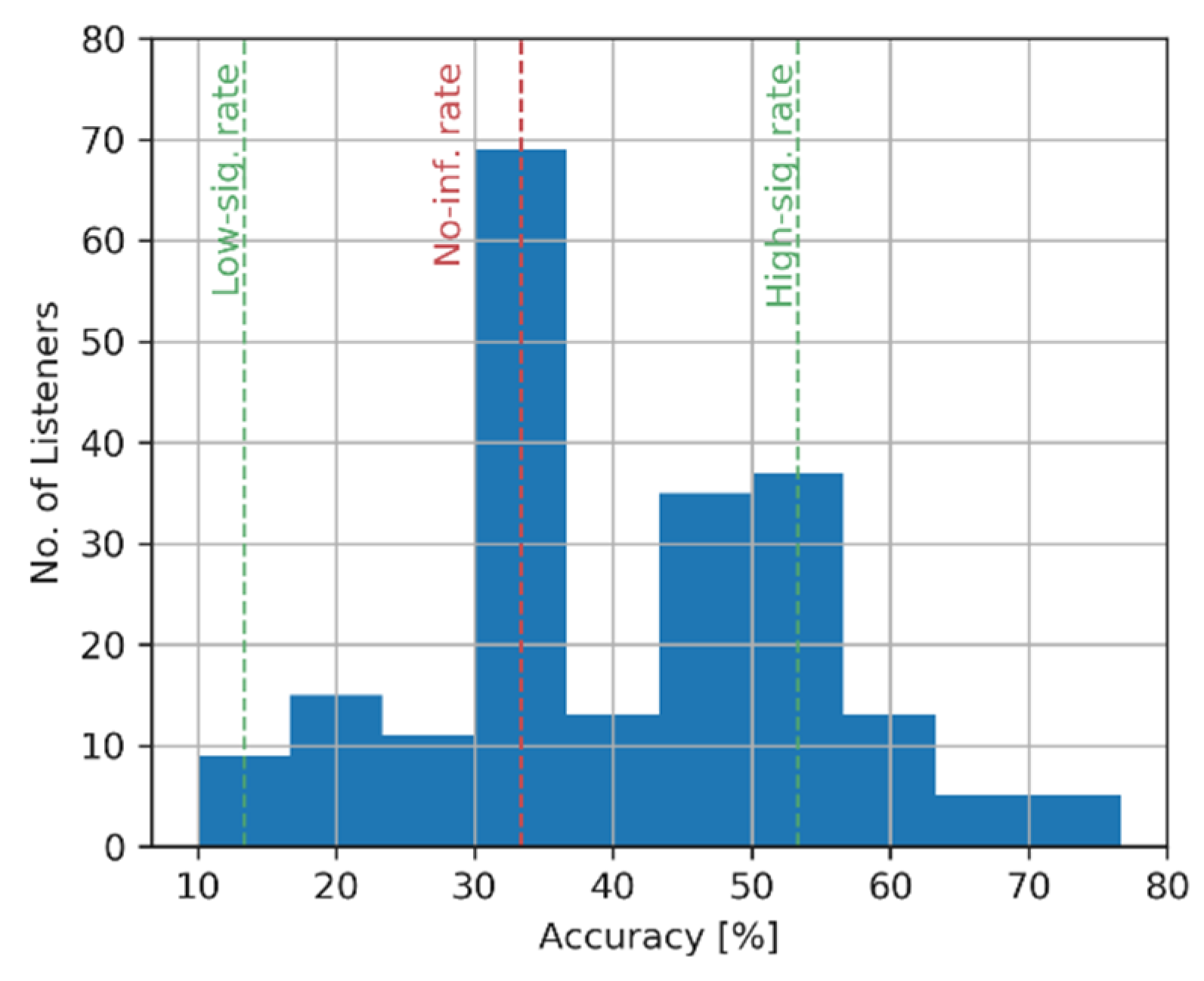
4.5. Listening Test Results
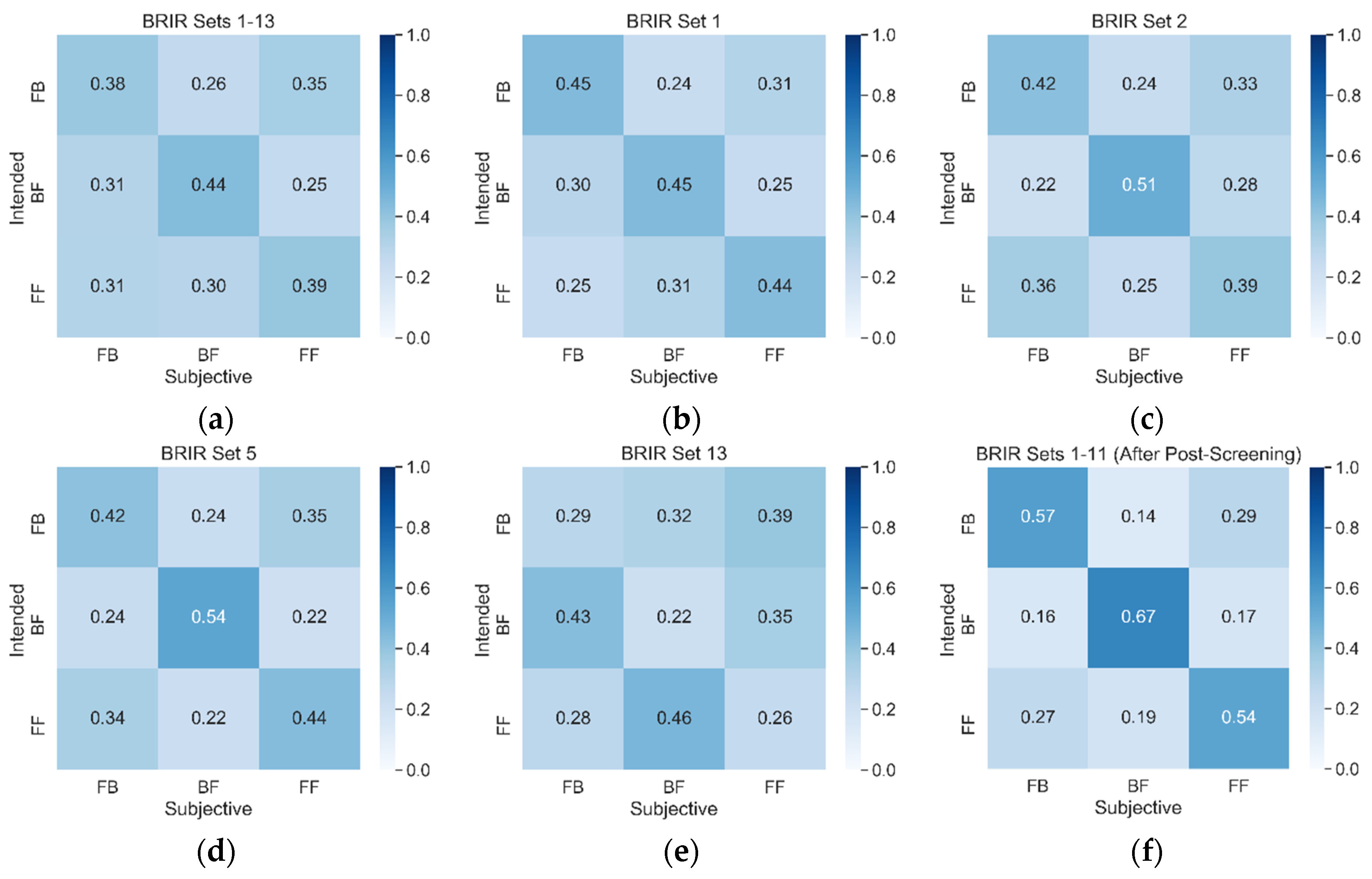
In total, all the listeners made 6360 classifications (212 listeners × 30 classifications). The listening test results were analyzed in terms of the classification “accuracy,” defined as the percentage ratio of the correct classifications to the total number of classifications made. As a correct classification, we considered a case whereby, for a given stimulus, the scene designated by a listener matched the intended scene during its binaural synthesis. We deliberately used the term “intended” instead of “actual” as, ultimately, it is the listeners who decide how the scenes are perceived.
According to the raw results, the overall classification rate exhibited by the listeners was low, being equal to 40.6%. This outcome is only slightly greater than the no-information rate (an accuracy level resulting from classifying the scenes by chance), which in our experiment amounted to 33.3%. This was an unsurprising outcome, since front–back discrimination, involved during the scene classification, is a challenging task under the static head scenario and also considering all the confounding electro-acoustical factors, including uncontrolled background noise, uncontrolled headphones frequency response, and no free-field headphone compensation. Nevertheless, due to a large number of classifications made, the above result is statistically significant at p = 10−33 level according to the binomial test.
The confusion matrix obtained for the raw data is shown in Figure 2a. It confirms the erratic nature of the results, with the accuracy levels along a diagonal axis only slightly exceeding the no-information rate. Confusion matrices obtained for the stimuli synthesized using individual BRIR sets are quantitatively similar to the above one. Therefore, for clarity, the confusion matrices for only three selected BRIR sets (1, 2, and 5) are presented in panels b-d of that figure. In contrast to the above results, the confusion matrix obtained for BRIR set 13 appeared to be slightly different. This is presented in panel e. Visual inspection of that matrix indicates that the listeners tended to misclassify BF scenes as FB and FF scenes as BF. This unusual effect was also confirmed later in the statistical post-hoc test accompanying the analysis of variance (see below).
The accuracy scores were also calculated for each listener and inspected in the form of a histogram presented in Figure 3, showing the distribution of the listeners’ accuracy scores. It can be seen that the accuracy of the listeners ranged from 10% to almost 80%. The main peak in the histogram indicates that almost 70 listeners exhibited very poor performance, approximately equal to the no-information rate (33.3%), highlighting the need for some form of post-screening of the data. Another group of approximately 70 listeners (the second peak in the histogram) showed a better classification performance, ranging from 45% to 65%. Low and high statistical significance rate levels, equal to 13.3% and 53.3%, respectively, were also included in the histogram (green vertical lines). They were estimated based on the binomial test performed at a 0.05 significance level. The data from all the listeners whose scores lay between these two rates could not be considered as statistically significant. This does not mean that their data are meaningless, as the statistical significance depends on the number of classifications made and, consequently, when the data from all the listeners are combined, the statistical sensitivity of the experimental protocol substantially increases (as it was already demonstrated above in relation to the classification accuracy from the all listeners). Out of 212 listeners, only 48 had accuracy scores exceeding the high significance rate. The data from these listeners were later retained in the post-screening procedure (see below). Surprisingly, one outlying listener had a score below the low-significance rate, implying that he or she consistently misclassified some scenes.
The histogram discussed above showed the listeners’ scores lumped for all the BRIR sets, hence obscuring any inter-BRIR effects. To investigate how the accuracy scores varied between the stimuli synthesized using individual BRIR sets, they were also plotted in the form of boxplots across all BRIR sets, as illustrated in Figure 4a. The outcomes confirmed the previous observations. Namely, for almost all BRIR sets, the scores barely exceeded the no-information rate of 33.3%. Due to a large number of observations, the deviation from the no-information rate was statistically significant, except for BRIR sets 3, 7, 8, and 12, according to a double-sided t-test performed at 0.05 significance level. Interestingly, for a BRIR set 13, the accuracy scores were statistically different from the no-information rate but in the opposite direction. In this case, the mean accuracy score was statistically significantly less than 33.3%, confirming the above observation about the consistent misclassification of the scenes, as illustrated earlier in Figure 2e.
Analysis of variance (ANOVA) test was carried out in order to formally investigate the inter-BRIR effects formerly seen in Figure 4a. The assumptions underlying the ANOVA model were positively verified using the omnibus test of homogeneity of variance and Jarque–Bera test of the assumption of normality. The obtained ANOVA model was statistically significant, F(12,199) = 3.28, p = 2.39 × 10⁻⁴. However, according to the results of the post hoc Tukey HSD test, no statistical differences between the mean accuracy scores across the BRIR sets were detected, with the exception of a BRIR set 13, which was statistically different from the other ones. This outcome further supports the observation about the outlying nature of the data obtained for BRIR 13.
The exact reason for the outlying characteristics of the data obtained using a BRIR set 13 is unknown. The above BRIR set was acquired in the Audio Laboratory at the University of Rostock, which was also the case for a BRIR set 12 (see Table 2). However, in the latter case, the results are not as outlying as the ones obtained using BRIR 13. Nevertheless, after excluding the outlying BRIR set 13, the results obtained using a BRIR set 12 are the worst of all the BRIR sets, with the mean accuracy of 33.96%, being almost equal to the no-information rate.
In contrast to the stimuli synthesized using BRIR sets 1-11, the stimuli synthesized with BRIR sets 12 and 13 were generated employing a simulated wave-field synthesis model [13]. The outlying or poor results gathered for BRIR sets 12 and 13 could have resulted from signal processing artifacts pertinent to a wave-field synthesis (e.g., spatial aliasing). Hence, considering their commonalities in terms of the origin and the signal processing algorithm used, it was decided to remove (post-screen) the data obtained both for BRIR set 12 and 13.

4.6. Post-Screening

Following from above, the post-screening procedure involved the two following steps:
  • removing the data obtained using BRIR sets 12 and 13 (as a result, the accuracy increased from 40.6% to 42.5%),
  • retaining the data obtained only from the listeners whose accuracy scores were no less than the statistical significance threshold of 53.3%, resulting in the further accuracy rise to 59.7%.
The results obtained after the post-screening procedure are shown in Figure 4b. It can be seen that the scores markedly improved, as the mean accuracy scores increased to almost 60%. This improved score is used in the remainder of the paper as a basis for comparison with the classification accuracy obtained by the machine-listening algorithm
While some variations in the scores can be seen across the BRIR sets in Figure 4b, the ANOVA model was not statistically significant. Hence, despite the visual variations seen in the figure, no inferences regarding the inter-BRIR effects could be made.
The confusion matrix, obtained after completing the above post-screening procedure, is presented in Figure 2f. In contrast to the matrices shown in the remaining panels of that figure, distinct maxima along the diagonal line seem to emerge.

5. Classification Performed by Machine Learning Algorithms

5.1. Selection of the Algorithms

At the outset of this study, it was planned to compare the performance of human listeners against that of CNN only, assuming that this deep learning algorithm would substantially outperform the traditional classification methods. The outcomes of the pilot tests, however, not only undermined this assumption but also showed that for some conditions, the CNN and traditional algorithms could complement each other (for some groups of recordings CNN may show strong performance whereas traditional techniques may exhibit weaknesses and vice versa). Therefore, it was decided to include in this study both the deep learning technique based on CNN as well as the three traditional machine learning algorithms, namely SVM, XGBoost, and Logit. SVM and XGBoost algorithms represent the state-of-the-art traditional classification methods, whereas Logit was included here for its simplicity and a possibility of using L1 regularization [42], which is advantageous from the viewpoint of feature selection.

5.2. Development and Test Datasets

In our previous study with the traditional machine-listening algorithm [13], we used 4368 excerpts for training and another group of 1560 excerpts for testing purposes, encompassing all 13 BIRIR sets, as explained earlier in Section 3 (Table 1). Since in this study it was decided to remove the data associated with BRIR sets 12 and 13, the repositories intended for training and testing were reduced to 3696 and 1320 items, respectively. Note that for consistency of comparison between human and machine-listening tests, the same group of 1320 binaural audio excerpts intended for “testing” was used both in the listening tests (after post-screening) and in the experiments described in this section.

5.3. Convolutional Neural Network

The best-performing deep learning algorithms in such areas as acoustic scene classification or audio event recognition still exploit fixed spectrogram signal representations rather than learnable signal transformations [43]. Therefore, a former approach was also adopted in this study. To this end, the binaural audio recordings were converted to spectrograms and then fed to the input of CNN.

5.3.1. Spectrograms extraction

Drawing inspiration from the work of Han et al. [27], four spectrograms were extracted from each binaural audio recording. The first two spectrograms were calculated from the left (l) and right (r) channel signals, respectively. The remaining two spectrograms were computed accordingly from the sum (m = l + r) and difference signals (s = lr). While it could be argued that the latter two spectrograms are redundant as they do not introduce any new information, they might facilitate the network training process and hence improve its performance, as indicated in our pilot study [14].
Mel-frequency spectrograms are commonly exploited in the deep learning algorithms used for speech recognition, acoustic scene classification or audio event recognition [27,31,43,44]. While Mel-frequency spectrograms offer a better resolution at low frequencies, it is unclear whether such a type of spectrogram is still superior in terms of “spatial” audio scene classification. According to the results of our pilot experiment (omitted here due to space limitations), CNN fed with linear-frequency spectrograms yielded slightly better results compared to those obtained with Mel-frequency spectrograms. Therefore, only linear-frequency spectrograms were used in this study.
The temporal resolution of the spectrograms was set to 40 ms with a 50% overlap. Hence, for the recordings of 7 s in duration used in this study, each spectrogram contained 349 time frames. A Hamming window was applied to the signals in each frame. The number of frequency bands in the spectrograms was set to 150 since according to the outcomes of our pilot experiment [14], such a number of frequency bands provides a reasonable trade-off between the classification accuracy and the computational load imposed on the network. The low- and high-frequency limits of both types of spectrograms were set to 700 Hz and 16 kHz, respectively (extending the frequency range beyond those limits brought little benefit in the CNN performance). The range of the spectrogram values was limited (clipped) to 90 dB relative to the peak value.
The image resolution of the spectrograms was equal to 150 × 349 pixels (number of frequency-bands × number of time-frames). The spectrograms were combined into three-dimensional tensors and then fed to the network input. The size of each tensor was equal to 150 × 349 × Nch, where Nch represented the number of channels retained in a tensor. In this study, the number of channels Nch was equal to four, since each binaural recording was represented by four spectrograms.
In summary, every audio recording was converted to four spectrograms, with the resolution of 150 × 349 pixels each. According to the typical practice in the area of machine learning [27,44], the spectrograms were standardized prior to their use by the convolutional network. The spectrograms were calculated in MATLAB using a VOICEBOX toolbox [45].

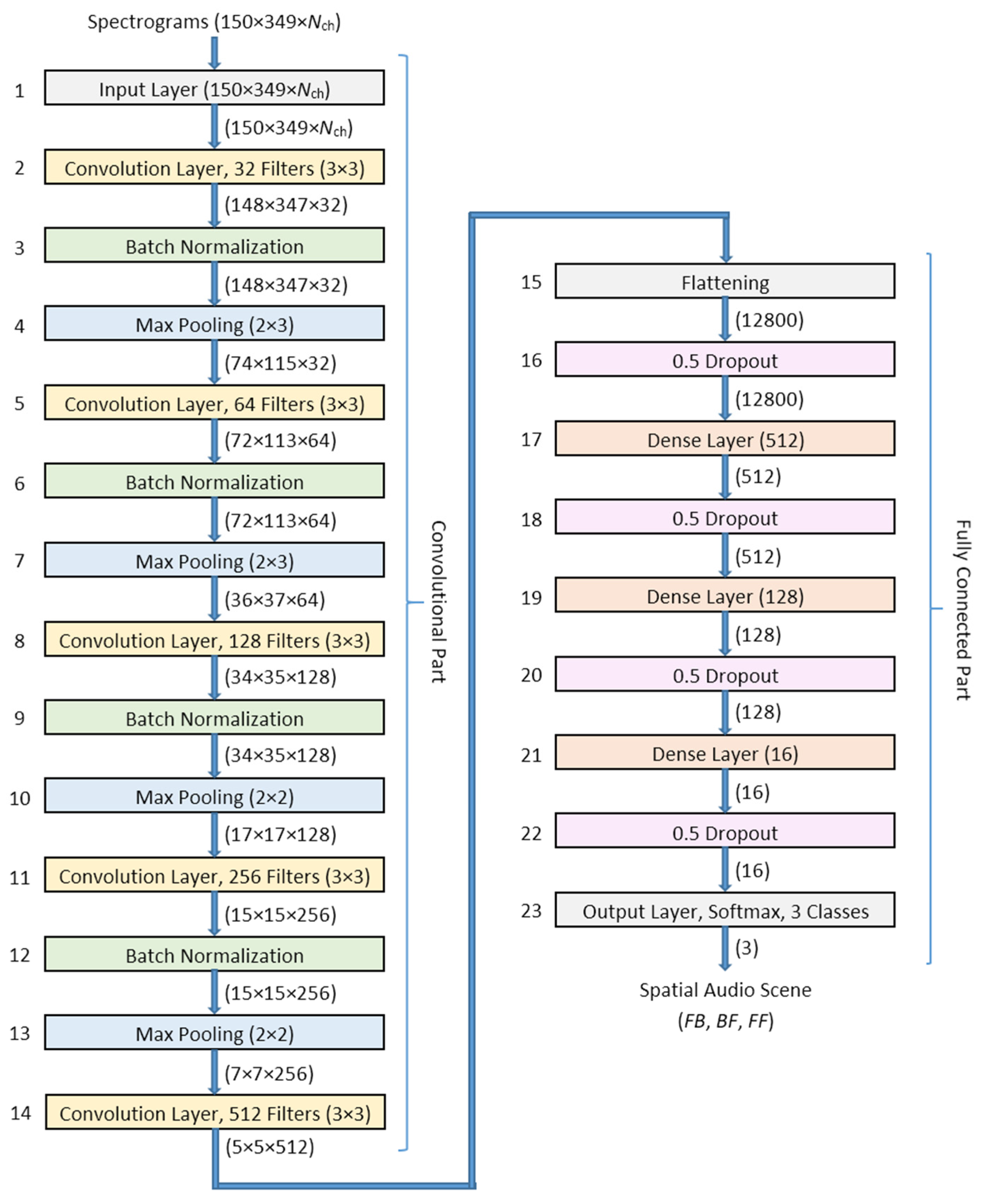
5.3.2. Convolutional Neural Network Topology

Due to a relatively small database employed in this study, it was decided to design the convolutional neural network based on the well-proven AlexNet architecture [46]. The layout of the proposed network is depicted in Figure 5. Out of the 23 layers used in the network, the first 14 are responsible for the spectrogram processing using the convolutional filters, whereas the remaining layers (15–23) constitute its fully connected part. The dimensions of the tensors processed by the network are indicated by the numbers in brackets, positioned at the interconnections between the adjacent layers.
Five convolutional layers were employed in the network (layers 2, 5, 8, 11, and 14). They all had the same kernel size of 3 × 3. The size of the kernel was selected according to our pilot test results [14]. In order to reduce the resolution of the processed spectrograms, four max pooling layers were employed (layers 4, 7, 10, and 13). Batch normalization was exploited after the first four convolutional layers to accelerate the learning procedure (layers 3, 6, 9, and 12). While the original resolution of the spectrograms used at the network input was gradually reduced from 150 × 349 to 5 × 5 pixels at the output of the last convolutional layer (layer14), the number of convolutional filters progressively increased in each consecutive convolutional layer, amounting to 32, 64, 128, 256, and 512, respectively. The above strategy, involving the increasing of a number of filters in subsequent convolutional layers, combined with a progressive reduction in the image resolution, is commonly applied in convolutional networks [46].
The two-dimensional spectrograms were converted into vectors in layer 15 and subsequently processed by the full connected dense layers consisting of 512, 128, and 16 nodes, respectively. Four dropout layers, with the dropout rate being equal to 0.5, were employed to prevent the network from overfitting (layers 16, 18, 20, and 22). The last layer was responsible for providing the results of the classification. A rectified linear unit was used in all the convolutional and dense layers, whereas a Softmax function was incorporated in the output layer.

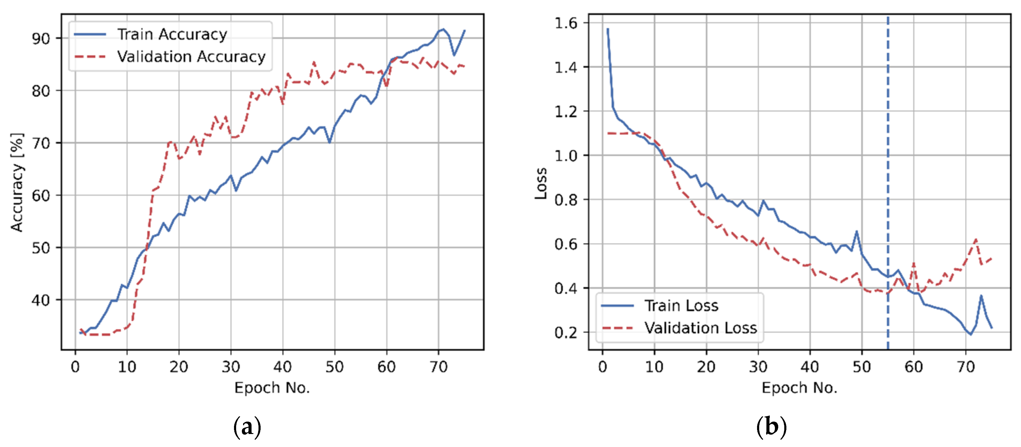
5.3.3. Convolutional Neural Network Training

In total, the network contained more than 8 million trainable parameters. The network was trained using the Adam [47] optimization technique with a categorical cross-entropy selected as a loss function. The learning rate was set to 1 × 10⁻⁴, whereas the batch size was adjusted to 128. The maximum number of training epochs was set to 200.
The network was trained until it started to overfit, with the early stopping algorithm implemented to reduce the computation time. To this end, approximately 90% of the training set was used to train the network, whereas the remaining 10% of the training set was employed for the validation purposes. Figure 6 demonstrates the learning curves for the training accuracy and training loss, respectively. It shows that while the train classification accuracy progressively increases (with some fluctuations across the training epochs), the validation accuracy saturates when the training algorithm completes approximately 60 epochs (Figure 6a), indicating a possible terminating epoch for the training procedure. However, instead of relying on the validation accuracy, in line with the typical practice in machine learning [48], the early stopping criterion was based on finding the minimum in the validation loss curve, as demonstrated in Figure 6b. In this example, the training procedure was terminated after 55 epochs.
The network was implemented in Python, using Keras, Tensorflow, scikit-learn and, NumPy packages. The computations were accelerated with a graphical processing unit (NVIDIA RTX 2080Ti).

5.4. Traditional Machine Learning Algorithms

The following three traditional algorithms were employed in this work: XBoost, SVM, and Logit. Two kernels were initially considered to be employed in the SVM classifier: linear and radial. According to the pilot results undertaken under the BRIR mismatched conditions (the testing procedure is described in detail below in Section 5.5), the test classification accuracy obtained for the SVM algorithm with the linear and radial kernels was equal to 54.1% and 53.3%, respectively, with no statistically significant difference between these results (t-test, p = 0.70). However, when the algorithm was tested under the BRIR matched conditions, the accuracy obtained for the linear and radial kernels equaled 78.4% and 83.8%, respectively, with the difference being statistically significant according to the t-test at p = 2.8 × 10⁻⁴ level. Therefore, in this study, only the radial kernel was employed in the SVM algorithm due to its superior accuracy performance.

5.4.1. Feature Extraction

All three traditional algorithms employed in this work (XBoost, SVM, and Logit) utilized at their input a set of features extracted using the procedure explained in detail in our previous study [13]. The set consisted of 1376 metrics, including binaural cues, spectral features, and Mel-frequency cepstral coefficients. For reproducibility, the feature set can be downloaded from [34]. The features were standardized before they were used in the training procedure.

5.4.2. Hyper-Parameters and Training

Each of the classification algorithms contained a number of hyper-parameters that needed to be tuned prior to their use in the training procedure. For the XGBoost classification algorithm, the number of estimators n had to be selected. In the case of the SVM, with a radial kernel (the type of a kernel was chosen in the pilot test), it was necessary to tune C and γ values. For the Logit algorithm (with the L1 regularization chosen to benefit from its inherent feature selection property), the C value had to be adjusted.
According to the results of the pilot test, out of the three traditional classification algorithms employed in this study, SVM was particularly sensitive to the number of features selected at its input, indicating the need for a formal feature selection procedure. To this end, the feature selection procedure was implemented, in which the importance of features was ranked according to the F-statistic derived from the ANOVA test. The number of selected features k constituted an additional hyper-parameter to be tuned. The above procedure was used only in combination with the SVM classification algorithm.
A standard grid search technique combined with a 10-fold cross-validation procedure was followed to adjust the hyper-parameters for each of the traditional algorithms prior to their training (such procedure could not be used earlier in the case of the CNN algorithm, since it would be too time-consuming, given the computation load of the CNN algorithm). The values of the hyper-parameters considered for selection in the grid-search algorithm, along with the selected values, are presented in Appendix B (see Table A1, Table A2 and Table A3, respectively).
The three traditional machine learning algorithms were implemented in Python ecosystem, using scikit-learn and NumPy packages. The XGBoost algorithm was accelerated with the help of a graphical processing unit—GPU (NVIDIA RTX 2080Ti).

5.5. Testing Procedure

Both the CNN and the three traditional machine learning algorithms (XGBoost, SVM, and Logit) were tested using a dedicated test set, as explained earlier in Section 5.2. Similarly to the results from the listening test, the performance of the machine learning algorithms was evaluated using the classification accuracy score and by a visual inspection of the confusion matrices.
In order to gauge how generalizable classification algorithms are, it is vital that they are trained and then tested under different conditions. Therefore, in this study, care was taken that different music content (artists, songs, albums) was used in the datasets employed for training and testing, respectively. While the training and test datasets were mutually exclusive in terms of the music content, there was some information “leakage” between them due to the fact that the same impulse responses (BRIR sets) were used to synthesize both groups of the recordings. Therefore, to get the fuller picture of the algorithm’s performance, they were tested under the two scenarios: BRIR matched and BRIR mismatched. The idea of testing the algorithms both under matched and mismatched impulse response conditions was also pursued by Wang et al. [25] in their recent study aiming to automatically identify the direction of the audio sources in binaural signals.
In the former scenario (BRIR matched testing), a single model is trained using the development dataset and then applied to the test set. Hence, the model is trained and tested with the recordings synthesized using the same eleven BRIR sets. Therefore, the term “BRIR matched testing” signifies the fact that the model is trained and tested under the same acoustic conditions (the same simulated rooms and dummy heads). In the latter scenario (BRIR mismatched testing), the models are trained and then tested with the stimuli synthesized using different BRIR sets. Hence, the models are tested under the acoustic conditions “unseen” during its training.
The advantage of BRIR matched testing is that it is less computationally demanding than the BRIR mismatched testing as it involves developing and testing only a single model but it may lead to overly “optimistic” results (inflated accuracy rates). On the other hand, BRIR mismatched testing is theoretically more reliable in terms of checking the generalizability of the algorithm, but it normally entails building and testing several models.
There are many ways in which the classification algorithms can be tested under the BRIR mismatched scenario. However, in line with the strategy taken in our former study [13], a leave-one-BRIR-out procedure was followed. In this procedure, eleven BRIR-specific models were trained and evaluated. Each model was trained using the stimuli synthesized with ten selected BRIR sets and then tested using the recordings synthesized with the single BRIR set which was left out during the training. This way, each model was tested on the stimuli synthesized with the BRIR set which was not “seen” by the model during its training.
Note that no distinction between matched and mismatched testing was made in the case of the classification task performed by human listeners. Humans undergo life-long training, being exposed to a variety of room acoustics and spatial audio scenes, providing them with the skills to localize ensembles of audio sources around their heads in unknown conditions. Since it is unlikely that the listeners, who took part in this experiment, were acquainted with the room acoustics represented by the BRIR sets used in this study (Table 2), it is safe to assume that the listening test was undertaken only under the BRIR mismatched conditions. It would be impractical to repeat the listening test under the BRIR matched conditions as it would require all the listeners to physically attend the venues listed in Table 2.
In contrast to the traditional machine learning algorithms, where the results are repeatable, in the case of the CNN algorithm, the classification results are slightly different each time the model is trained and tested (due to a very large number of the trainable parameters combined with inherent randomness of the neural network training procedure). Therefore, in the case of the CNN algorithm, the training and testing procedure was repeated ten times, with the mean classification accuracy values reported in the remained of the paper.

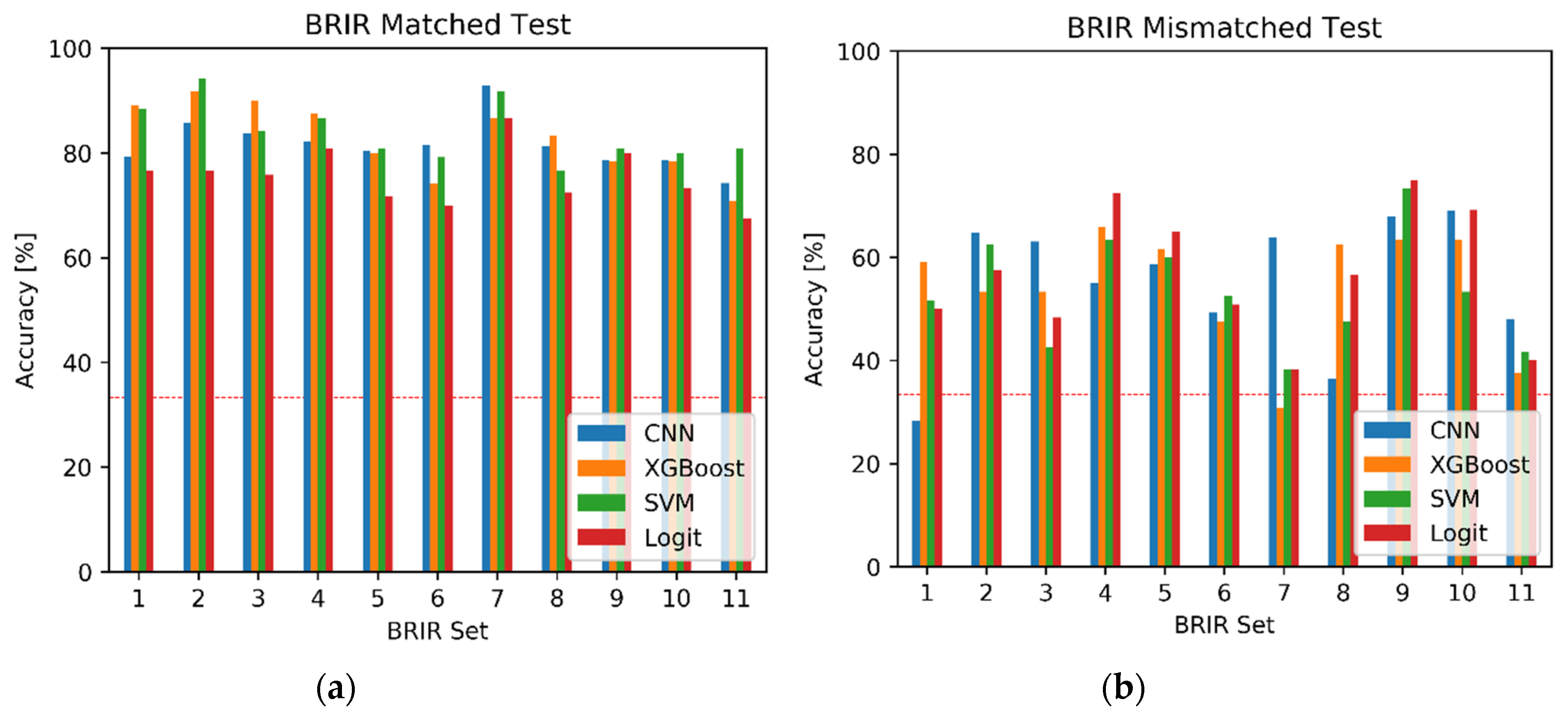
5.6. Results from Machine Learning Algorithms

The classification results obtained with the machine learning algorithms, both under BRIR matched and BRIR mismatched scenarios, are summarized in Figure 7. For comparison, the left pane of the figure shows the classification results reached by human listeners.
Under the BRIR matched test scenario, the SVM, XGBoost, and CNN algorithms performed equally well, with the classification accuracy being equal to 83.9%, 82.7%, and 81.7%, respectively, with no statistically significant differences between the results according to a t-test (p > 0.058). Logit was the worst performing algorithm, yielding an accuracy of 75.6%. The difference in the accuracy between the Logit algorithm and the above three algorithms was statistically significant at p < 9.2 × 10⁻⁶ level. The examples of the confusion matrices obtained for all four algorithms are presented in Figure 8a–d. They show that the algorithms are relatively good at the classification of the first two scenes (FB and BF) and slightly worse at the classification of the last scene (FF). The last two panes in Figure 8 illustrate the confusion matrices achieved for BRIR sets 2 and 7, respectively, demonstrating an exceptionally good BRIR-specific performance obtained using the SVM and CNN algorithms.
For the BRIR mismatched test scenario, the performance of all four algorithms markedly dropped down to the level of approximately 55%, with no statistically significant differences in performance between them (p > 0.085), as indicated by overlapping confidence intervals in Figure 7. The figure demonstrates that the outcomes of the experiment strongly depend on the testing method.
Figure 9 confirms the above observations, showing the confusion matrices obtained under the BRIR mismatched scenario. The first four panes of that figure illustrate the results obtained using CNN, XGBoost, SVM, and Logit algorithms, respectively. The confusion matrices are substantially worse than those obtained under the BRIR matched condition. The last two panes of Figure 9 show the BRIR-specific results. They illustrate the confusion matrices for BRIR set 9 achieved with the SVM and Logit algorithms, respectively. As before, visual inspection of these two confusion matrices confirms rather mediocre performance of the algorithms.
For completeness, Figure 10 shows the overview of the BRIR-specific results. While the differences in performance between the algorithms are rather small under the BRIR matched test (Figure 10a), they are much more pronounced under the BRIR mismatched scenario (Figure 10b). For example, CNN was markedly outperformed by the traditional algorithms for BRIR set 1 under the mismatched test condition (p < 1.3 × 10⁻⁵). However, its performance was superior for BRIR set 7 (p < 1.6 × 10⁻⁷), indicating that the strengths and weaknesses of the classification methods could be BRIR-specific.

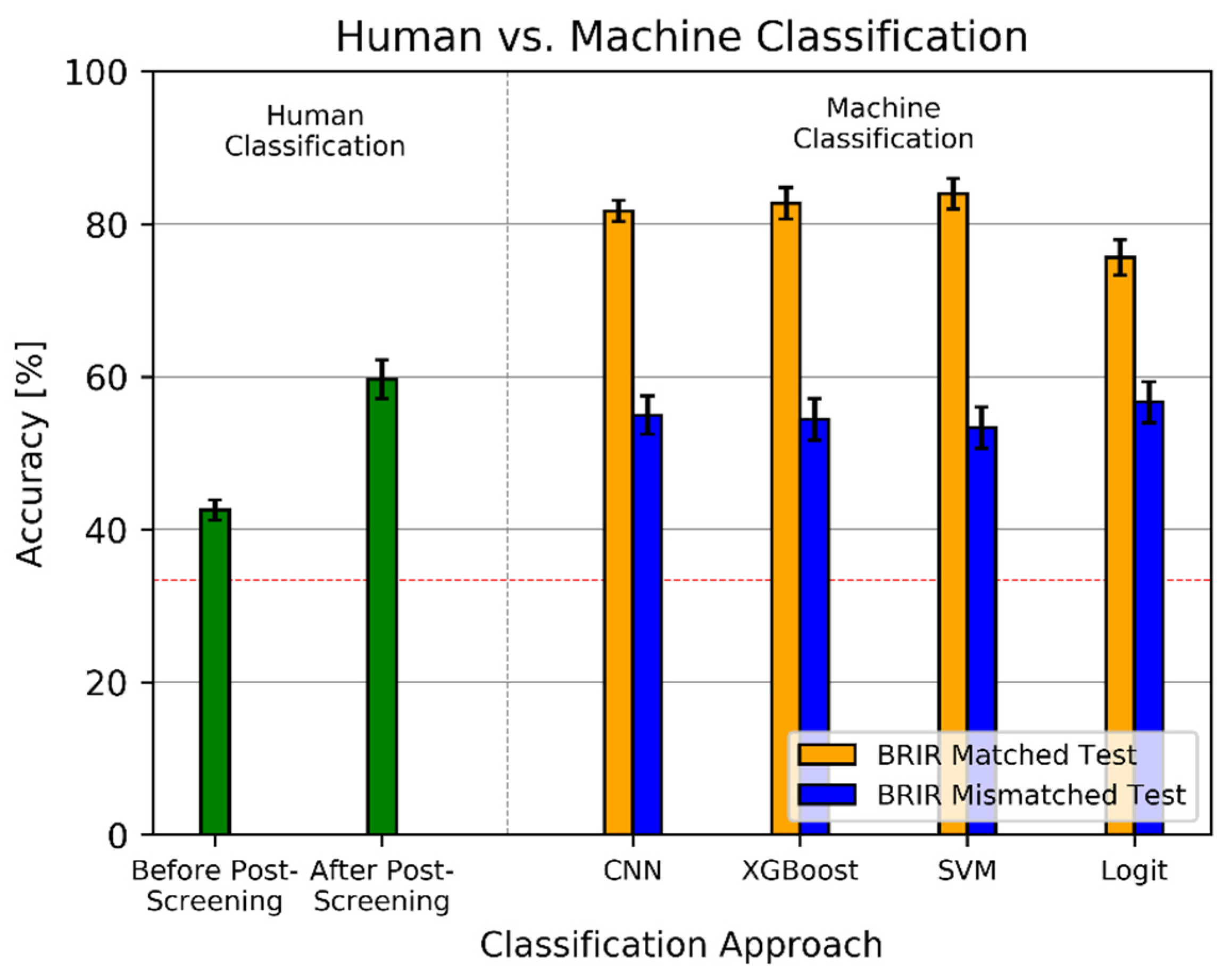
5.7. Comparison with the Listening Test Results

According to the obtained results presented earlier in Figure 7, for the BRIR matched test scenario, the machine learning algorithms markedly outperformed human listeners. The difference between the best performing algorithm (SVM) and the accuracy reached by the listeners who passed the post-screening test is equal to 24%. This difference is statistically significant at p = 1.2 × 10−47 level. For the worst performing algorithm (Logit), this difference is slightly reduced, amounting to 16%, but it is still statistically significant (p = 1.6 × 10⁻¹⁹). However, when the algorithms are tested under the BRIR mismatched scenario, the performance of the classification algorithms is similar or even slightly worse than that exhibited by the listeners who passed the post-screening test. For the Logit algorithm, the classification accuracy is equal to 56.7%, which constitutes a 3% drop in the accuracy compared to the level attained by the listeners who passed the post-screening test. Nevertheless, this difference is not statistically different (p = 0.11), and therefore the Logit algorithm cannot be regarded as performing worse than the listeners who passed the post-screening test. For the remaining three algorithms, this difference is greater (up to 6%) and statistically significant (p < 0.011). Hence, it could be concluded that the CNN, XGBoost, and SVM algorithms perform slightly worse than the listeners who passed the post-screening test under the BRIR mismatched test scenario.

6. Discussion

The accuracy reached by human listeners in the task of the classification of spatial audio scenes was low, being equal to 42.5% for all the listeners and to almost 60% for the listeners who passed the post-screening test. Such a low accuracy rate could be attributed to the difficulty faced by the listeners under the static-head scenario. The literature shows that the rate of front–back discrimination errors is large when the users of binaural audio systems cannot exploit the mechanism of the head movements [18]. Moreover, the classification task was also hindered by an uncontrolled electro-acoustical environment (background noise, headphones frequency response, no free-field headphone compensation). While this feature of the listening test could be considered as the significant limitation of the study, the obtained results represent a typical scenario of an ordinary listener auditioning binaural music recordings over the Internet under “realistic” conditions (enhanced ecological validity).
The outcome of the comparison between the classification accuracy reached by human listeners against those obtained by the machine audition algorithms depends on the way the algorithms are tested. Under the BRIR matched conditions, the classification algorithms outperform the listeners. However, under the BRIR mismatched conditions, the performance of the machine audition algorithms is comparable or even slightly worse than the level exhibited by the listeners who passed the post-screening test. Hence, the generalizability of the algorithms, understood as their ability to perform in unknown electro-acoustic conditions, needs to be further improved, which constitutes the direction for future work.
It is difficult to compare the results obtained using the machine learning algorithms with those reported in the literature, since the automatic classification of spatial audio scenes evoked by binaural audio recordings is a relatively new topic, constituting an emerging field of research. For the best performing algorithm (SVM), the classification results presented in this paper are 7% better than those obtained using a least absolute shrinkage and selection operator (LASSO) in our previous work [13] (p = 2.4 × 10⁻⁶), under the BRIR matched conditions. However, when the classification algorithms are tested under the BRIR mismatched scenario, the outcomes of this and the former study are almost identical, with the classification accuracy being equal to 56.7% and 56.8%, respectively (the difference is not statistically significant, p = 0.94).
The results obtained for the CNN algorithm appear to be somewhat disappointing as they are comparable to the outcomes obtained by the traditional algorithms (see Fig. 7). It was expected that this deep learning algorithm would substantially outperform the three traditional classification algorithms, since, in general, deep learning methods provide better accuracy performance than traditional machine learning classification algorithms [46]. One possible reason for the comparatively low performance of the CNN algorithm could be attributed to a relatively small training dataset, consisting of 3696 audio recordings, thus yielding 1232 training items per audio scene. Such a number of training items may be insufficient to train the network due to the risk of overfitting, considering the large number of its trainable parameters (more than 8 million). However, it is known that CNN algorithms are capable of reaching satisfactory classification results even when trained on relatively small datasets, containing 1000 items per class [48]. Moreover, the performance of the CNN algorithms can be further boosted by incorporating various forms of data augmentation [46,48]. According to the initial follow-up experiments, not reported in the paper due to space limitations, data augmentation based on the mix-up technique (generating new audio recordings by mixing the existing recording exhibiting the same spatial audio scenes) or involving a signal resampling technique (pitch shifting and time stretching) introduced only small improvements to the CNN performance, indicating that there is no “information gain” or any other network training benefit (e.g., reducing the overfitting effect), resulting from the artificial extension of the dataset by means of re-using the existing recordings in a modified form. Therefore, a more plausible explanation for the relatively poor performance of the CNN algorithm is that only eleven BRIR sets were used to generate the training dataset, hence limiting the “amount” of spatial acoustic information embedded into the training database and, consequently, preventing the algorithm from benefiting fully from its deep learning capabilities. Therefore, it could be hypothesized that extending the existing database by introducing new spatial audio information, e.g., by including audio recordings synthesized using new BRIR sets representing new electro-acoustic conditions (e.g., varied room acoustics and dummy heads) would improve the performance of the CNN algorithm.
According to the results, the CNN algorithm substantially outperformed the traditional algorithms for one of the considered BRIR sets. However, there was another BRIR set for which the opposite outcome was observed (see Section 5.6). Consequently, it may be argued that there are some audio characteristics which are not captured by the spectrograms and/or the CNN algorithm, while they are “picked up” by the traditional feature extraction algorithms combined with the traditional classification algorithms (and vice versa). The identification of these unique characteristics is planned to be undertaken in the follow-up work.
The calculation time required by the SVM, XGBoost, and Logit algorithms was approximately 4, 9, and 52 times shorter than computational time required by CNN algorithm, respectively, implying that the Logit algorithm is the least computationally demanding method (while still providing similar classification rates compared to the remaining methods), whereas the CNN algorithm imposes the highest computational load. However, the direct comparison of computation time might not reflect the actual computational load due to the fact that the CNN and XGBoost algorithms were GPU accelerated (NVIDIA RTX 2080Ti), whereas the remaining methods utilized the central processor unit (Intel Core i7-7820X CPU 3.6GHz).

7. Conclusions

The machine learning algorithms considered in this study (CNN, XGBoost, SVM, and Logit) outperformed human listeners in the task of the classification of the spatial audio scenes evoked by binaural music recordings under the BRIR matched scenario—that is, in the case where the algorithms were trained and tested using the signals synthesized with the same binaural room impulse responses. However, when the classification algorithms were applied to the signals generated using the impulse responses “unseen” during their training, the scenario referred to as the BRIR mismatched test, their performance was comparable or even slightly worse than that of the human listeners. Hence, the generalizability aspect of the machine algorithms needs to be further improved in order to be able to automatically outperform the listeners in unknown electro-acoustic conditions. The possible research directions for such enhancements are outlined in the paper.

Author Contributions

Conceptualization and methodology, S.K.Z. and H.L.; development of the web application, P.A. and O.D.; supervision of the listening tests, P.A. and O.D.; data analysis, S.K.Z.; design and implementation of the deep learning algorithm, S.K.Z.; paper writing, S.K.Z. and H.L. All authors have read and agreed to the published version of the manuscript.

Funding

The work was supported by the grant from Białystok University of Technology (WZ/WI-IIT/4/2020) and funded with resources for research by the Ministry of Science and Higher Education in Poland.

Acknowledgments

The authors are grateful to all the listeners who volunteered to participate in the listening tests.

Conflicts of Interest

The authors declare no conflict of interest.

Appendix A. Examples of The Headphones Models Used in the Listening Test

Examples of the headphones used in the listening test, as reported by the listeners (in alphabetical order):
  • AKG (K240 Monitor, K240 Studio, K272 HD, K550, K701, K712 Pro)
  • Apple (EarPods with lighting connection)
  • Asus (Cerberus)
  • Audio-Technica (ATH-M50, ATH-R70x)
  • Beyerdynamic (Custom One Pro, DT 331, DT-770 Pro 250 Ohm, DT-990 Pro 250 Ohm, T5p, Soul Byrd)
  • Bloody (G501)
  • Bose (QC25)
  • Canford Level Limited Headphones (HD480 88dBA)
  • Corsair (HS50, HS60)
  • Creative SoundBlaster (JAM)
  • Focal (Spirit Professional)
  • Genesis (Argon 200, H44, HM67, Radon 720)
  • HTC (HS S260)
  • Huawei (AM116)
  • HyperX (Cloud Alpha, Cloud 2)
  • ISK (HD9999)
  • Jabra Elite (65t)
  • JBL (E65BTNC, T110, T450BT, T460BT)
  • Klipsch Reference On-Ear Bluetooth Headophones, Koss (KSC75)
  • Logitech (G633, G933)
  • Mad Dog (GH702)
  • Nokia (WH-108)
  • Panasonic (RP-HJE125E-K, RP-HT161)
  • Philips (SHL3060BK)
  • Pioneer (SE-M531, SE-M521)
  • Razer (Kraken 7.1 Chroma, Kraken Pro v2, Thresher Tournament Edition)
  • Roccat Syva (ROC-14-100)
  • Samsung (EHS61)
  • Sennheiser (CX 300-II, HD 201, HD 215, HD 228, HD 280 PRO, HD 380 Pro, HD 4.40, HD 555, HD 559, HD 598)
  • Skullcandy (Uprock)
  • SMS (Studio Street by 50 Cent Wireless OverEar)
  • Snab Overtone (EP-101m)
  • Sony (MDR-AS200, MDR-EX110LPB.AE, MDR-E9LPB, MDR-NC8, MDR-ZX110B, MDR-XB550, MDR-XB950B1, WH-1000XM3)
  • SoundMagic (E10, E11)
  • Stax (404 LE)
  • Superlux (HD660, HD669, HD681)
  • Takstar (HD2000)
  • Thinksound (MS02)
  • Tracer (Gamezone Thunder 7.1, Dragon TRASLU 44893)
  • Urbanears, QCY (T2C)

Appendix B. Overview of the Hyper-Parameters in Traditional Machine Learning Algorithms

Table A1. Hyper-parameter values considered in the grid-search algorithm.
Classification AlgorithmHyper-Parameters
XGBoostnumber of estimators n = {100, 200, 500}
SVMnumber of features 1 k = {500, 700, 1376}
C = {1, 10, 100}
γ = {7.27 × 10⁻³, 7.27 × 10⁻⁴, 7.27 × 10⁻⁵}
LogitC = {0.01, 0.1, 1}
1 Feature selection was incorporated for SVM only.
Table A2. Hyper-parameter selected for the model used under the BRIR matched test conditions.
Classification AlgorithmHyper-Parameters
XGBoostn = 100
SVMk = 700, C = 100, γ = 7.27 × 10⁻⁴
LogitC = 0.1
Table A3. Hyper-parameter selected for the eleven models used under the BRIR mismatched test conditions.
Classification AlgorithmHyper-ParameterBRIR Set Left Out during the Training
1234567891011
XGBoostn500500500500500500500500100500500
SVMk500500500500500500700500700700500
C100100101001001001001010010100
γ = 7.27×10−410−410−410−410−410−410−410−410−410−410−4
LogitC0.10.10.10.10.10.10.10.10.10.10.1

References

  1. Begault, D.R. 3-D Sound for Virtual Reality and Multimedia; NASA Center for AeroSpace Information: Hanover, MD, USA, 2000.
  2. Blauert, J. The Technology of Binaural Listening; Springer: Berlin, Germany, 2013. [Google Scholar]
  3. Roginska, A. Binaural Audio through Headphones. In Immersive Sound. The Art and Science of Binaural and Multi-Channel Audio, 1st ed.; Routledge: New York, NY, USA, 2017. [Google Scholar]
  4. Parnell, T. Binaural Audio at the BBC Proms, BBC R&D. Available online: https://www.bbc.co.uk/rd/blog/2016-09-binaural-proms (accessed on 14 July 2017).
  5. Firth, M. Developing Tools for Live Binaural Production at the BBC Proms, BBC R&D. Available online: https://www.bbc.co.uk/rd/blog/2019-07-proms-binaural (accessed on 7 February 2020).
  6. Kelion, L. YouTube Live-Streams in Virtual Reality and adds 3D Sound, BBC News. Available online: http://www.bbc.com/news/technology-36073009 (accessed on 18 April 2016).
  7. Zieliński, S.; Rumsey, F.; Kassier, R. Development and Initial Validation of a Multichannel Audio Quality Expert System. J. Audio Eng. Soc. 2005, 53, 4–21. [Google Scholar]
  8. MacPherson, E.A.; Sabin, A.T. Binaural weighting of monaural spectral cues for sound localization. J. Acoust. Soc. Am. 2007, 121, 3677–3688. [Google Scholar] [CrossRef] [PubMed]
  9. Benaroya, E.L.; Obin, N.; Liuni, M.; Roebel, A.; Raumel, W.; Argentieri, S.; Benaroya, L. Binaural Localization of Multiple Sound Sources by Non-Negative Tensor Factorization. IEEE/ACM Trans. Audio Speech Lang. Process. 2018, 26, 1072–1082. [Google Scholar] [CrossRef]
  10. Rumsey, F. Spatial quality evaluation for reproduced sound: Terminology, meaning, and a scene-based paradigm. J. Audio Eng. Soc. 2002, 50, 651–666. [Google Scholar]
  11. Zieliński, S.K. Spatial Audio Scene Characterization (SASC). Automatic Classification of Five-Channel Surround Sound Recordings According to the Foreground and Background Content. In Multimedia and Network Information Systems, Proceedings of the MISSI 2018; Advances in Intelligent Systems and Computing; Springer: Cham, Switzerland, 2019. [Google Scholar]
  12. Zielinski, S.; Lee, H. Feature Extraction of Binaural Recordings for Acoustic Scene Classification. In Proceedings of the 2018 Federated Conference on Computer Science and Information Systems; Polish Information Processing Society PTI: Warszawa, Poland, 2018; Volume 15, pp. 585–588. [Google Scholar]
  13. Zieliński, S.K.; Lee, H. Automatic Spatial Audio Scene Classification in Binaural Recordings of Music. Appl. Sci. 2019, 9, 1724. [Google Scholar] [CrossRef] [Green Version]
  14. Zielinski, S. Improving Classification of Basic Spatial Audio Scenes in Binaural Recordings of Music by Deep Learning Approach. In Proceedings of the Bioinformatics Research and Applications; Springer Science and Business Media LLC: New York, NY, USA, 2020; pp. 291–303. [Google Scholar]
  15. He, K.; Zhang, X.; Ren, S.; Sun, J. Delving Deep into Rectifiers: Surpassing Human-Level Performance on ImageNet Classification. In Proceedings of the 2015 IEEE International Conference on Computer Vision, Santiago, Chile, 7–13 December 2015; pp. 1026–1034. [Google Scholar] [CrossRef] [Green Version]
  16. Zonoz, B.; Arani, E.; Körding, K.P.; Aalbers, P.A.T.R.; Celikel, T.; Van Opstal, A.J. Spectral Weighting Underlies Perceived Sound Elevation. Nat. Sci. Rep. 2019, 9, 1–12. [Google Scholar] [CrossRef] [PubMed] [Green Version]
  17. Blauert, J. Spatial Hearing. The Psychology of Human Sound Localization; The MIT Press: London, UK, 1974. [Google Scholar]
  18. Begault, D.R.; Wenzel, E.M.; Anderson, M.R. Direct Comparison of the Impact of Head Tracking, Reverberation, and Individualized Head-Related Transfer Functions on the Spatial Perception of a Virtual Speech Source. J. Audio Eng. Soc. 2001, 49, 904–916. [Google Scholar] [PubMed]
  19. Jeffress, L.A. A place theory of sound localization. J. Comp. Physiol. Psychol. 1948, 41, 35–39. [Google Scholar] [CrossRef] [PubMed]
  20. Breebaart, J.; van de Par, S.; Kohlrausch, A. Binaural processing model based on contralateral inhibition. I. Model structure. J. Acoust. Soc. Am. 2001, 110, 1074–1088. [Google Scholar] [CrossRef] [PubMed] [Green Version]
  21. May, T.; Ma, N.; Brown, G.J. Robust localisation of multiple speakers exploiting head movements and multi-conditional training of binaural cues. In Proceedings of the IEEE International Conference on Acoustics, Speech and Signal Processing (ICASSP), Institute of Electrical and Electronics Engineers (IEEE), Brisbane, Australia, 19–24 April 2015; pp. 2679–2683. [Google Scholar]
  22. Ma, N.; Brown, G.J. Speech localisation in a multitalker mixture by humans and machines. In Proceedings of the INTERSPEECH 2016, San Francisco, CA, USA, 8–12 September 2016; pp. 3359–3363. [Google Scholar] [CrossRef] [Green Version]
  23. Ma, N.; May, T.; Brown, G.J. Exploiting Deep Neural Networks and Head Movements for Robust Binaural Localization of Multiple Sources in Reverberant Environments. IEEE/ACM Trans. Audio Speech Lang. Process. 2017, 25, 2444–2453. [Google Scholar] [CrossRef] [Green Version]
  24. Ma, N.; Gonzalez, J.A.; Brown, G.J. Robust Binaural Localization of a Target Sound Source by Combining Spectral Source Models and Deep Neural Networks. IEEE/ACM Trans. Audio Speech Lang. Process. 2018, 26, 2122–2131. [Google Scholar] [CrossRef]
  25. Wang, J.; Wang, J.; Qian, K.; Xie, X.; Kuang, J. Binaural sound localization based on deep neural network and affinity propagation clustering in mismatched HRTF condition. EURASIP J Audio Speech Music Process. 2020, 4. [Google Scholar] [CrossRef] [Green Version]
  26. Vecchiotti, P.; Ma, N.; Squartini, S.; Brown, G.J. End-to-end binaural sound localisation from the raw waveform. In Proceedings of the IEEE International Conference on Acoustics, Speech and Signal Processing (ICASSP), Brighton, UK, 12–17 April 2019; pp. 451–455. [Google Scholar]
  27. Han, Y.; Park, J.; Lee, K. Convolutional neural networks with binaural representations and background subtraction for acoustic scene classification. In Proceedings of the Conference on Detection and Classification of Acoustic Scenes and Events 2017, Munich, Germany, 16 November 2017; pp. 1–5. [Google Scholar]
  28. Raake, A. A Computational Framework for Modelling Active Exploratory Listening that Assigns Meaning to Auditory Scenes—Reading the World with Two Ears. Available online: http://twoears.eu (accessed on 8 March 2019).
  29. Szabó, B.T.; Denham, S.L.; Winkler, I. Computational models of auditory scene analysis: A review. Front. Neurosci. 2016, 10, 1–16. [Google Scholar] [CrossRef] [PubMed] [Green Version]
  30. Barchiesi, D.; Giannoulis, D.; Stowell, D.; Plumbley, M.D. Acoustic scene classification: Classifying environments from the sounds they produce. IEEE Signal. Process. Mag. 2015, 32, 16–34. [Google Scholar] [CrossRef]
  31. Wu, Y.; Lee, T. Enhancing Sound Texture in CNN-based Acoustic Scene Classification. In Proceedings of the IEEE International Conference on Acoustics, Speech and Signal Processing (ICASSP), Brighton, UK, 12–17 May 2019; pp. 815–819. [Google Scholar]
  32. Woodcock, J.; Davies, W.J.; Cox, T.J.; Melchior, F. Categorization of Broadcast Audio Objects in Complex Auditory Scenes. J. Audio Eng. Soc. 2016, 64, 380–394. [Google Scholar] [CrossRef]
  33. Lee, H.; Millns, C. Microphone Array Impulse Response (MAIR) Library for Spatial Audio Research. In Proceedings of the 143rd AES Convention, New York, NY, USA, 8 October 2017. [Google Scholar]
  34. Zieliński, S.K.; Lee, H. Database for Automatic Spatial Audio Scene Classification in Binaural Recordings of Music. Zenodo. Available online: https://zenodo.org (accessed on 7 April 2020).
  35. Satongar, D.; Lam, Y.W.; Pike, C.H. Measurement and analysis of a spatially sampled binaural room impulse response dataset. In Proceedings of the 21st International Congress on Sound and Vibration, Beijing, China, 13–17 July 2014; pp. 13–17. [Google Scholar]
  36. Stade, P.; Bernschütz, B.; Rühl, M. A Spatial Audio Impulse Response Compilation Captured at the WDR Broadcast Studios. In Proceedings of the 27th Tonmeistertagung—VDT International Convention, Cologne, Germany, 20 November 2012. [Google Scholar]
  37. Wierstorf, H. Binaural Room Impulse Responses of a 5.0 Surround Setup for Different Listening Positions. Zenodo. Available online: https://zenodo.org (accessed on 14 October 2016).
  38. Werner, S.; Voigt, M.; Klein, F. Dataset of Measured Binaural Room Impulse Responses for Use in an Position-Dynamic Auditory Augmented Reality Application. Zenodo. Available online: https://zenodo.org (accessed on 26 July 2018).
  39. Klein, F.; Werner, S.; Chilian, A.; Gadyuchko, M. Dataset of In-The-Ear and Behind-The-Ear Binaural Room Impulse Responses used for Spatial Listening with Hearing Implants. In Proceedings of the 142nd AES Convention, Berlin, Germany, 20–23 May 2017. [Google Scholar]
  40. Erbes, V.; Geier, M.; Weinzierl, S.; Spors, S. Database of single-channel and binaural room impulse responses of a 64-channel loudspeaker array. In Proceedings of the 138th AES Convention, Warsaw, Poland, 7–10 May 2015. [Google Scholar]
  41. Zieliński, S.K. On Some Biases Encountered in Modern Audio Quality Listening Tests (Part 2): Selected Graphical Examples and Discussion. J. Audio Eng. Soc. 2016, 64, 55–74. [Google Scholar] [CrossRef]
  42. James, G.; Witten, D.; Hastie, T.; Tibshirani, R. An Introduction to Statistical Learning with Applications in R; Springer: London, UK, 2017. [Google Scholar]
  43. Abeßer, J. A Review of Deep Learning Based Methods for Acoustic Scene Classification. Appl. Sci. 2020, 10, 2020. [Google Scholar] [CrossRef] [Green Version]
  44. Rakotomamonjy, A. Supervised Representation Learning for Audio Scene Classification. IEEE/ACM Trans. Audio Speech Lang. Process. 2017, 25, 1253–1265. [Google Scholar] [CrossRef]
  45. Brookes, M. VOICEBOX: Speech Processing Toolbox for MATLAB. Available online: http://www.ee.ic.ac.uk/hp/staff/dmb/voicebox/voicebox.html (accessed on 17 April 2020).
  46. Krizhevsky, A.; Sutskever, I.; Hinton, G.E. ImageNet classification with deep convolutional neural networks. Commun. ACM 2017, 60, 84–90. [Google Scholar] [CrossRef]
  47. Kingma, D.P.; Ba, J. Adam: A Method for Stochastic Optimization. Available online: https://arxiv.org/abs/1412.6980 (accessed on 26 August 2020).
  48. Chollet, F. Deep Learning with Python; Manning Publications: Shelter Island, NY, USA, 2020. [Google Scholar]
Figure 1. Graphical user interface exploited in the developed web application: (a) excerpt from the instructions for the listeners; (b) interface used for spatial audio scene classification.
Applsci 10 05956 g001
Figure 2. Examples of confusion matrices obtained from human listeners: (a) All data; (b) BRIR set 1; (c) BRIR set 2; (d) BRIR set 5; (e) BRIR set 13; (f) BRIR sets 1-11 (data after post-screening). Vertical axis represents the classification results obtained from the listeners whereas the vertical axis denotes the scenes as intended during the procedure of the binaural synthesis of the audio recordings.
Applsci 10 05956 g002
Figure 3. Histogram of the accuracy scores calculated for each listener.
Applsci 10 05956 g003
Figure 4. Boxplots of the accuracy scores for stimuli synthesized using specific BRIR sets: (a) before post-screening; (b) after post-screening. Red line denotes no-information rate.
Applsci 10 05956 g004
Figure 5. Topology of the convolutional neural network used for the spatial audio scene classification.
Applsci 10 05956 g005
Figure 6. Example learning curves of the convolutional neural network: (a) accuracy; (b) loss. A vertical blue line denotes the training termination point.
Applsci 10 05956 g006
Figure 7. Comparison of human against machine classification of spatial audio scenes. Red line denotes no-information rate. Error bars represent 95% confidence intervals.
Applsci 10 05956 g007
Figure 8. Examples of confusion matrices obtained using machine learning algorithms under BRIR matched conditions: (a) convolutional neural network CNN, BRIR sets 1-11; (b) extreme gradient boosting framework (XGBoost), BRIR sets 1-11; (c) support vector machine (SVM), BRIR sets 1-11; (d) logistic regression (Logit), BRIR sets 1-11; (e) SVM BRIR set 2; (f) CNN, BRIR set 7. Vertical axis represents the classification results obtained from the classification algorithms.
Applsci 10 05956 g008
Figure 9. Examples of confusion matrices obtained under BRIR mismatched conditions: (a) CNN, BRIR sets 1-11; (b) XGBoost, BRIR sets 1-11; (c) SVM, BRIR sets 1-11; (d) Logit, BRIR sets 1-11; (e) SVM BRIR set 9; (f) Logit, BRIR set 9. Vertical axis represents the classification results obtained from the classification algorithms.
Applsci 10 05956 g009
Figure 10. Classification accuracy obtained using the machine learning algorithms: (a) BRIR matched scenario; (b) BRIR mismatched scenario. Red line denotes no-information rate.
Applsci 10 05956 g010
Table 1. Constitution of the binaural audio repository (adapted from [34]).
DestinationNo. of Multitrack RecordingsNo. of BRIR SetsNo. of Binaural Excerpts
Training112134368
Testing40131560
Table 2. The binaural-room-impulse-response (BRIR) sets used in the study (adapted from [13]).
No.DescriptionDummy HeadRT60 (s)
1Salford, British Broadcasting Corporation (BBC)—Listening Room [35]B&K HATS Type 41000.27
2Huddersfield—Concert Hall [33]Neumann KU1002.1
3Westdeutscher Rundfunk (WDR) Broadcast Studios—Control Room 1 [36]Neumann KU1000.23
4WDR Broadcast Studios—Control Room 7 [36]Neumann KU1000.27
5WDR Broadcast Studios—Small Broadcast Studio (SBS) [36]Neumann KU1001.0
6WDR Broadcast Studios—Large Broadcast Studio (LBS) [36]Neumann KU1001.8
7Technische Universität (TU) Berlin—Calypso Room [37]KEMAR 45BA0.17
8TU Ilmenau—TV Studio (distance of 3.5 m) [38]KEMAR 45BA0.7
9TU Ilmenau—TV Studio (distance of 2 m) [39]KEMAR 45BA0.7
10TU Ilmenau—Listening Laboratory [39]KEMAR 45BA0.3
11TU Ilmenau—Rehabilitation Laboratory [39]KEMAR 45BANA
12University of Rostock—Audio Laboratory (additional absorbers) [40]KEMAR 45BA0.25
13University of Rostock—Audio Laboratory (all broadband absorbers) [40]KEMAR 45BA0.31

