Classification of Dermoscopy Skin Lesion Color-Images Using Fractal-Deep Learning Features

Featured Application

Detection of skin diseases is one of today’s priority tasks worldwide. Computer-aided diagnosis is a promising tool for prevention (diagnosis).

Abstract

The detection of skin diseases is becoming one of the priority tasks worldwide due to the increasing amount of skin cancer. Computer-aided diagnosis is a helpful tool to help dermatologists in the detection of these kinds of illnesses. This work proposes a computer-aided diagnosis based on 1D fractal signatures of texture-based features combining with deep-learning features using transferred learning based in Densenet-201. This proposal works with three 1D fractal signatures built per color-image. The energy, variance, and entropy of the fractal signatures are used combined with 100 features extracted from Densenet-201 to construct the features vector. Because commonly, the classes in the dataset of skin lesion images are imbalanced, we use the technique of ensemble of classifiers: K-nearest neighbors and two types of support vector machines. The computer-aided diagnosis output was determined based on the linear plurality vote. In this work, we obtained an average accuracy of 97.35%, an average precision of 91.61%, an average sensitivity of 66.45%, and an average specificity of 97.85% in the eight classes’ classification in the International Skin Imaging Collaboration (ISIC) archive-2019.

1. Introduction

Due to the changes in the environmental conditions in which we currently live, we observe that more people suffer some form of cancer [1]. For example, ultraviolet radiation (UV) is one of the primary risk factors for skin cancer. In 1975, Fitzpatrick proposed a scale from I to VI of how the skin type reacts to UV [1]. Type I are the very fair skins (more susceptible to developing some form of skin cancer), and Type VI comprises intensely pigmented dark brown skins (less affected). Hence, this kind of illness is most frequent in countries with a predominantly fair skin population. Nowadays, in Ireland, the skin cancer’s diagnosis is over 11,000 cases per year. Most people living in Ireland have fair skin, which means skin type I or II on the Fitzpatrick scale. Ireland’s government, concerned about the rising incidence of skin cancer, in its National Cancer Strategy (2019–2022), prioritizes the need to implement a national skin cancer prevention plan [2]. In the USA annually, skin cancer diagnosis surpasses five million cases [3]. Globally, in 2010, skin diseases were the fourth leading cause of nonfatal illnesses that caused economic losses due to inabilities [4].

Abnormal growth of skin cells could develop skin cancer. One of the first warning signs is that skin lesions, like new moles, bumps, sores, scales, or dark spots, grow and do not go away. Mainly, skin cancer divides into two categories, melanoma and non-melanoma (basal cell carcinoma and squamous cell carcinoma) [5]. The dermatologists employ the ABCDE criteria in the diagnosis of skin lesions: asymmetry (A), border (B), color (C), differential structure (D), and evolving (E) [6]. In the asymmetry feature, the dermatologist searches if the lesion is uneven. The border characteristic measures the ragged edges. The color analysis determines if the spot has an unusual coloration. The diameter parameter measures if the spot is more extensive than one-quarter inch. The evolving features indicate if the lesion is changing in size, color, or shape. Therefore, the dermatologist analyses the form, appearance, and color of the mole or spot. Detection of skin diseases is one of today’s priority tasks worldwide. Characterizing the role that the textures play in skin diseases will help us develop more robust computer-aided diagnosis methods.

In recent years, neural networks have once again boomed in a wide variety of applications. By obtaining satisfactory results, these become a promising tool for the classification of skin lesions. CNNs are based on the convolution operation of the image with different filters, offering extensive and varied information. In its first layers, CNNs get the lines and edge features, while in the deeper layers, they find more specific details in the images. It is well known that the convolution operation is not invariant to geometric transformations like translation, rotation, and scale [7]. That is why neural networks require a large number of training images to extract all the possible ways that the image can have, hence their high computational cost. In addition, images of skin lesions can have low contrast between the lesion and healthy skin, which could interfere with the correct segmentation of the lesions [8]. That can lead to loss of valuable information that could be used for proper classification of the injury. Due to these aspects, in this work, it is proposed to complement the Densenet-201 network’s information with the compact information obtained from fractal signatures, which extract global and local information from the images considering the three color bands, R, G, B.

2. Related Works

The texture is an essential part of the aspect of the skin surface. For this reason, texture-based techniques have been developed. These methods are based on statistical analysis, spectral analysis, and fractal dimension, among others. The statistical approach uses pixels distributions [8,9,10,11,12,13,14,15,16,17,18,19,20,21,22]. In the spectral methods, the patterns are analyzed in the frequency domain [23,24,25,26,27,28]. The fractal dimension framework evaluates image complexity [29,30].

The techniques of texture-based extraction have been applied to myriad problems, achieving excellent results in multi-class classification [31,32]. However, the skin lesion classification task is so complex that most proposals are based on the two-class classification problem [33,34,35,36,37,38,39]. Because melanoma is deadly cancer, most of those works are focused on identifying it. Few works present systems that classify more than two types of skin lesions [40,41,42,43,44,45], like Wu et al. [42], that use five convolutional neural networks to classify face skin lesions of the Xiangya-Derm database. They selected 2656 face images of seborrheic keratosis, actinic keratosis, rosacea, lupus erythematosus, basal cell carcinoma, and squamous cell carcinoma. The network Inception-ResNet-v2 yielded the best results, a recall (or sensitivity) of 67.2%, and a 63.7% precision.

This proposal presents a computer-aided diagnosis methodology to discriminates between the eight skin lesion classes: actinic keratosis (AK), basal cell carcinoma (BCC), squamous cell carcinoma (SCC), benign keratosis (BKL), melanoma (MEL), melanocytic nevus (NEV), dermatofibroma (DER), and the vascular lesion (VASC).

3. Background

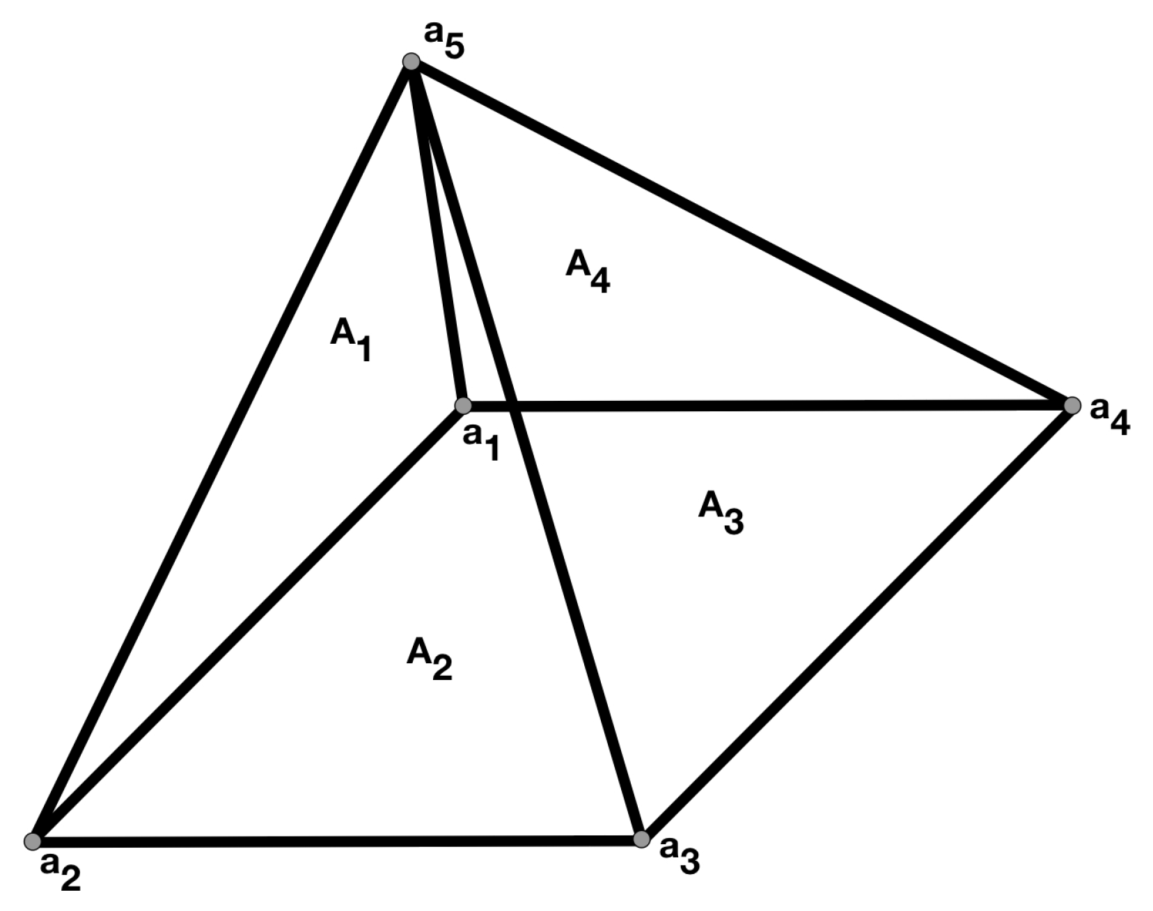
The Fractal Signature of Texture Images

The fractal term arose from the works of Benoit Mandelbrot when he studied irregular geometric structures repeated at different scales [46]. The fractal objects have irregular shapes in which the standard measures cannot determine their dimension [47]. The fractal dimension pinpoints how the fractal object fills space as the measurement unit is refined. Generally, the fractal dimension is a fractional number instead of an integer number, as the point, the straight line, the square, and the cube have dimensions zero, one, two, and three. The skin lesions present irregular borders, so it is natural to measure their size with the fractal dimension. Moreover, Wahba et al. [41] recommended to include the fractal dimension in the ABCDE rule.

Recently, Backes et al. [48] proposed a texture signature based on the volumetric fractal dimension (Bouligand–Minkowski descriptor) to identify plants. On the other hand, Florindo et al. [49] used the Bouligand–Minkowski descriptors to pinpoint histological images of odontogenic keratocyst, a jaw cyst type. In this work, we propose to use fractal signatures obtained from triangular prisms [50]. Let $I(x,y)$ represent a gray-scale image of size $M\times N$. The fractal signature of $I(x,y)$ builds by

$$F\left(\delta \right)=\sum _{x=1}^{M-\epsilon }\sum _{y=1}^{N-\epsilon }{A}_{x,y}^{\alpha }\left(\delta \right),$$

(1)

where $\delta =1,2,\dots ,\lfloor {log}_2\left(min(M,N)\right)\rfloor$, and

$$A_{x,y}^{\alpha }\left(\epsilon \right)={(A_1+A_2+A_3+A_4)}^{\alpha },$$

(2)

is the addition of the four triangles’ area-values of the prism in Figure 1. $\alpha$ is a weight term for the sum of the area of the faces. The triangular prism, with a square base of length $\epsilon +1$, is obtained from the vertices: $a_1=\left(x,y,I(x,y)\right)$, $a_2=\left(x+\epsilon ,y,I(x+\epsilon ,y)\right)$, $a_3=\left(x+\epsilon ,y+\epsilon ,I(x+\epsilon ,y+\epsilon )\right)$, $a_4=\left(x,y+\epsilon ,I(x,y+\epsilon )\right)$, and $a_5=\left(x+\frac{\epsilon }{2},y+\frac{\epsilon }{2},z\right)$, with $z=\frac{I(x,y)+I(x+\epsilon ,y)+I(x,y+\epsilon )+I(x+\epsilon ,y+\epsilon )}{4}$, see Figure 1.

The addition of the areas of the triangular faces of all prisms built from $\epsilon =2$ and for all $(x,y)$ of the image, corresponds to the fractal signature, F, in its first index; that is, $F^{\alpha }\left(1\right)={\sum }_{x=1}^{M-2}{\sum }_{y=1}^{N-2}{A}_{x,y}^{\alpha }\left(2\right)$. The next square-base size is given by $\epsilon =4$, thus $F^{\alpha }\left(2\right)={\sum }_{x=1}^{M-4}{\sum }_{y=1}^{N-4}{A}_{x,y}^{\alpha }\left(4\right)$, and so on. The scalar $\epsilon$ is an even value of the form,

$$\epsilon =2^{\delta }.$$

(3)

Figure 2b shows the graph of $F_R,F_G,F_B$, the fractal signatures of the RGB dermoscopy color-image of the actinic keratosis of $450\times 600$ pixels in Figure 2a. Because of $min\{450,600\}$, $\delta =1,2,\dots ,\lfloor {log}_2\left(450\right)\rfloor =1,2,\dots ,\lfloor 8.8138\rfloor =1,2,\dots ,8$.

Thus, the three fractal signatures have length 8. Figure 2b exhibits three signatures with the same behavior. Due to the scale range of the graphs in Figure 2b, the three signatures look similar, but they are different in values, Figure 2c. The magnitude of the maximum values of the difference between the fractal signatures are: $max\left\{\right|F_R-F_G\left|\right\}=2.05\times {10}^7,max\left\{\right|F_R-F_B\left|\right\}=4.20\times {10}^7,max\left\{\right|F_G-F_B\left|\right\}=2.16\times {10}^7$.

Most of the aided-computer diagnosis try to reproduce what a dermatologist would do. The dermatologist gives a score to the segmented skin lesion’s ABCDE features [6]. The final result is the addition of the scores given. Based on a threshold value applied to the final result, the lesion is determined or not like a disease.

Commonly, aided-computer methodologies comprehend of four steps: segmentation, feature extraction, feature score, and classification [34]. An adequate segmentation must completely separate the healthy region from the diseased skin; however, in most of these images, it is not possible to have proper segmentation. These kinds of images have not very well-defined edges. In some cases, they present low contrast between the regions of the healthy and the diseased skin. That complicates the segmentation process and causes wrong segmentation of the lesion. In References [51,52], different state-of-the-art segmentation algorithms were tested, which in many cases could not make correct discrimination of healthy skin and diseased skin, mainly in the images of actinic keratosis and basal cell carcinoma. That caused it not to consider significant sections of the injuries. With fractal signatures we work with the whole image.

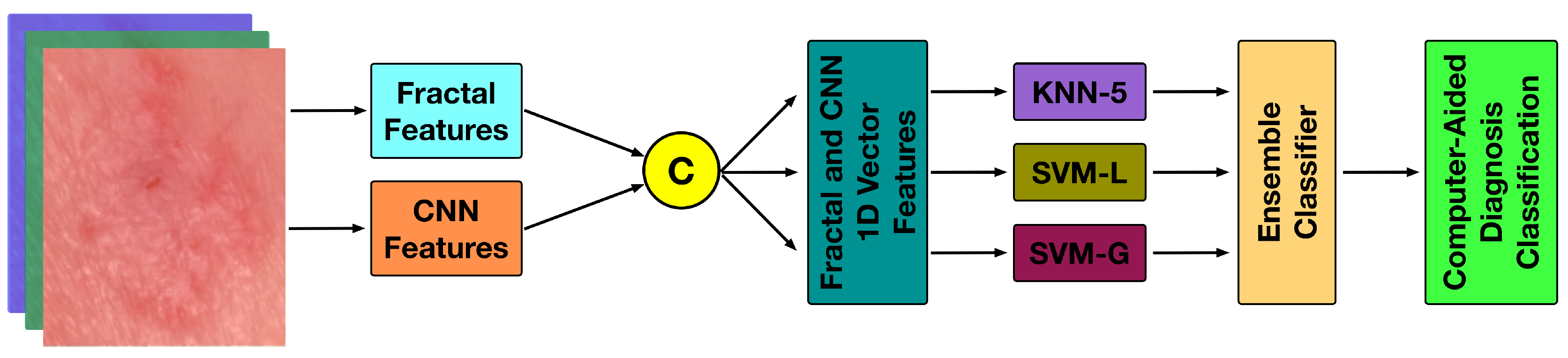
4. The Proposed Methodology

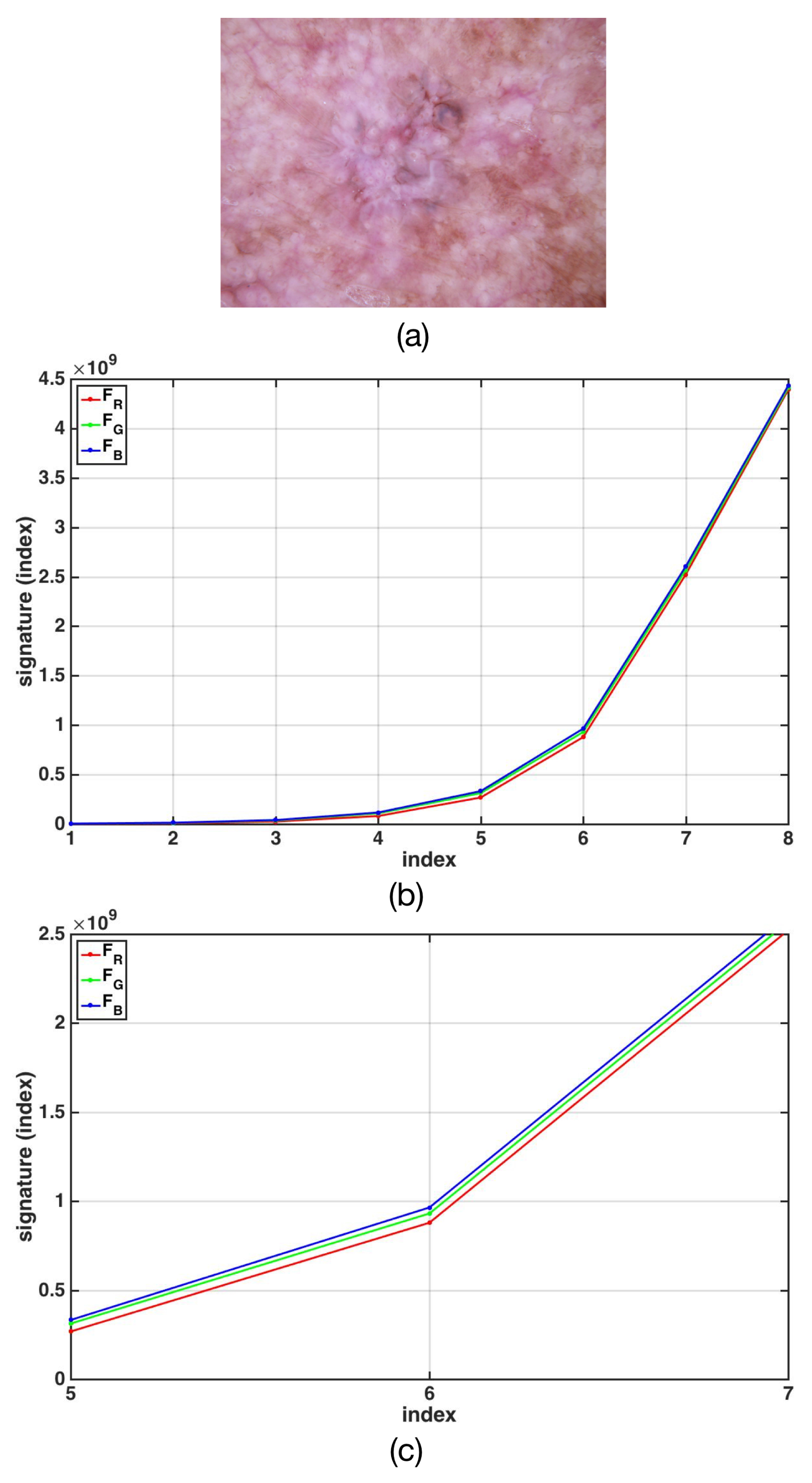
4.1. The Fractal Signature Features

Since we are working with images of different sizes, the fractal signatures are of different sizes. To avoid the size of the uneven signatures, we work with the energy $E_k$, the variance ${\sigma }_k^2$, and the entropy $H_k$ of the signatures [53], computed like

$$\begin{array}{ccc}\hfill E_k& =& \sum _{j=1}^n{F}_k^2\left(j\right),\hfill \end{array}$$

(4)

$$\begin{array}{ccc}\hfill {\sigma }_k^2& =& \frac{1}{n-1}\sum _{j=1}^n{\left(F_k\left(j\right)-{\overline{F}}_k\right)}^2,\hfill \end{array}$$

(5)

$$\begin{array}{ccc}\hfill H_k& =& -\sum _{j=1}^n\left[F_k\left(j\right)·{log}_2\left(F_k\left(j\right)\right)\right],\hfill \end{array}$$

(6)

where ${\overline{F}}_k$ is the mean of $F_k$, $k=R,G,B$, and n is the length of signature $F_k$, Equation (1).

Because the color of the lesion is one of the features in the ABCDE rule, it is imperative to preserve the color information of the images. Hence, the energy, variance, and entropy of the three signatures of the image, one signature per RGB color-channel, compose the image’s fractal signature, in the following manner.

$$\begin{array}{c}\hfill S_F=\left[E_R,E_G,E_B,{\sigma }_R^2,{\sigma }_G^2,{\sigma }_B^2,H_R,H_G,H_B\right].\end{array}$$

(7)

As the fractal signatures have different lengths, to have feature vectors of the same length, we decided to use the following statistical features: energy, variance, and entropy. The energy measures the signature’s strength. The variance measures the spread or dispersion of the signal around its mean value, and the entropy is the expected information content of the signal [53]. These three features obtained from each of the three 1D fractal signatures were added to the 100 deep-features extracted from the DenseNet-201. If the signal is viewing as a histogram, more statistical features could be explored like: skewness, kurtosis, mode, interquartile range, percentiles [21]. In addition, the statistical features obtained from grey level co-occurrence matrices (GLCMs, 2D signals) could be adapted to 1D signals [9,11,21]. That will be studied in the next step of this work.

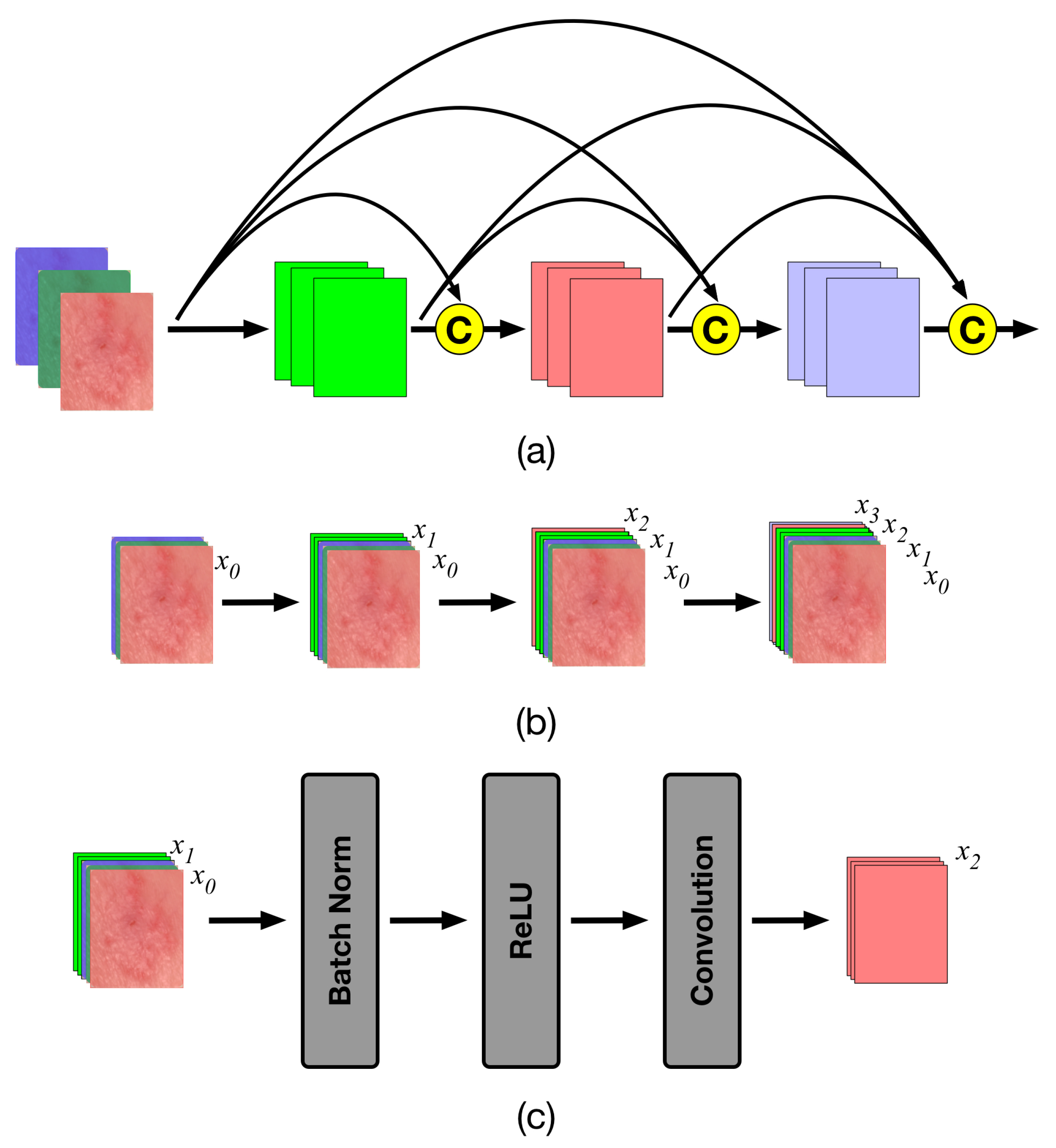
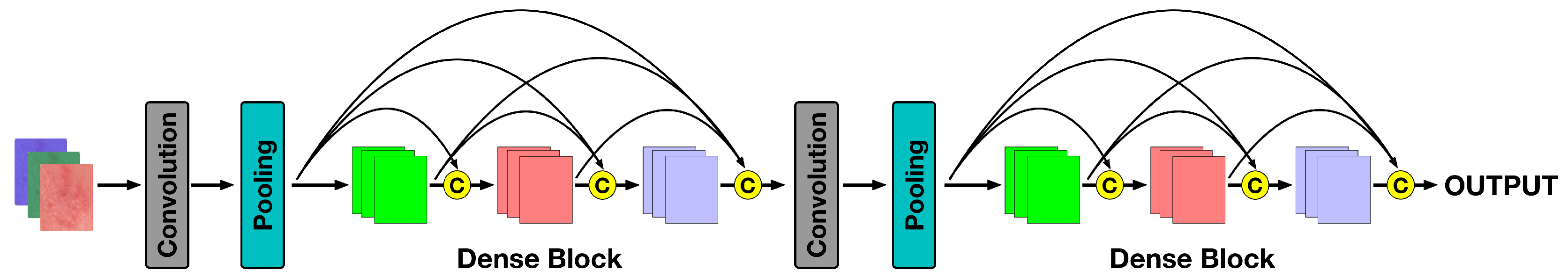
4.2. The Densenet Features

This proposal consists of a hybrid methodology that combines the features from fractal signatures with those obtained with the DenseNet-201 neural convolutional network. Like other neural networks, the DenseNets, in its first layers, get the lines and edge features, while in the deeper layers, it finds more specific details in the images [54]. DenseNet-201 was selected because it demonstrated handling better the smooth boundaries, like the skin lesion images [54]. The DenseNets connect all layers in a feed-forward form, Figure 3a. Hence, each layer gets additional input from all previous tiers and passes its feature-maps to subsequent layers. Instead of summing the features before they are moving into a layer, the DenseNet concatenates them. That results in a denser connectivity pattern in each of the layers, Figure 3b. The number of additional channels in each layer is named the growth rate; we use 32.

For each composition layer, pre-activation Batch Norm, ReLU (rectified linear units), and $3\times 3$ convolution (with stride 1) are utilized in each channel, that operations generated a new output feature-map, Figure 3c. In the Batch Norm layer, values in the activation matrix are divided by the sum of values in the kernel matrix. This is done to have all values between 0 and 1.The ReLu activation function yields to the CNN the non-linearity feature. It is widely used because it handles the vanishing gradient problem properly. In addition, it has the capability to train the network with higher computational efficiency [8]. The Rectified Linear Unit layer (ReLu) is defined as,

$$\varphi \left(x\right)=max(0,x)=\left\{\begin{array}{cc}x,& x\ge 0,\\ 0,& x0.\end{array}\right.$$

(8)

The DenseNet uses multiple dense blocks with transition layers, Figure 4. First, it uses a convolution layer of size $7\times 7$ with stride 2, followed by a max-pooling layer of $3\times 3$ with stride 2. Between two contiguous dense blocks, it employs a convolution layer of size $1\times 1$ with pace 1 followed by an average-pooling layer of size $2\times 2$ with stride 2. This proposal uses four dense blocks. The DenseNet-201 requires resizing the input images to $224\times 224$ pixels per channel. We use the MatLab 2019b function augmentedImageDatastore, which utilizes the scale’s affine transformation [55]. We selected to apply the bilinear interpolation operation, because between the nearest-neighbor, bilinear, and bicubic methods, it is the one that provides satisfactory results without spending as much time as the bicubic method does [55]. The output of the DenseNet-201 is a vector of length 100, called 1D CNN vector features, and denoted by $S_{CNN}$.

4.3. The Classifier Space

We use three classifier spaces, the K-nearest neighbor (KNN), and two support vector machines (SVM): linear and Gaussian kernels [56,57,58].

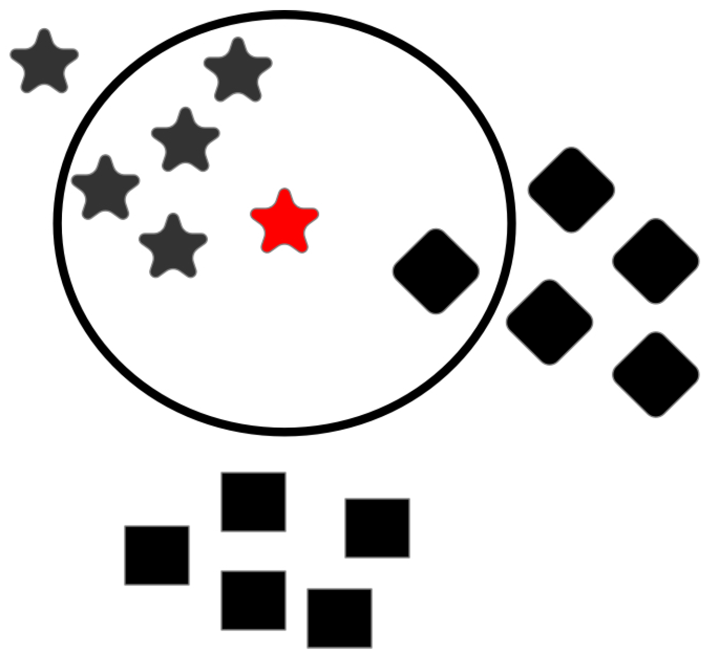
4.3.1. K-Nearest Neighbor

This is a non-probabilistic classifier [57]. It is popular due to its simplicity and excellent performance. For this type of classifiers, we have N training vectors ${\mathbf{x}}_j=[S_F,S_{CNN}]\in \{C_1,C_2,C_3,C_4,C_5,C_6,C_7,C_8\}$, that is, ${\mathbf{x}}_j$ is the concatenation of the fractal vector features $S_F$ and the CNN vector features $S_{CNN}$, $j=1,2,\dots ,N$, and $\{C_1,C_2,C_3,C_4,C_5,C_6,C_7,C_8\}$ is the finite set of skin lesion classes. To determine the class of the unknown vector features $\mathbf{x}$, we find the K points that are closest to $\mathbf{x}$. The majority class amongst these neighbors is the class assigned to $\mathbf{x}$. In this work, we use $K=5$, and we called it KNN-5. The Euclidean distance is used to compute the distance between the training data ${\mathbf{x}}_j$ and the unknown point $\mathbf{x}$, given by

$$d({\mathbf{x}}_j,\mathbf{x})=\sqrt{\sum _{i=1}^{109}{\left[{\mathbf{x}}_j\left(i\right)-\mathbf{x}\left(i\right)\right]}^2},$$

(9)

where $j=1,2,\dots ,N$, Figure 5.

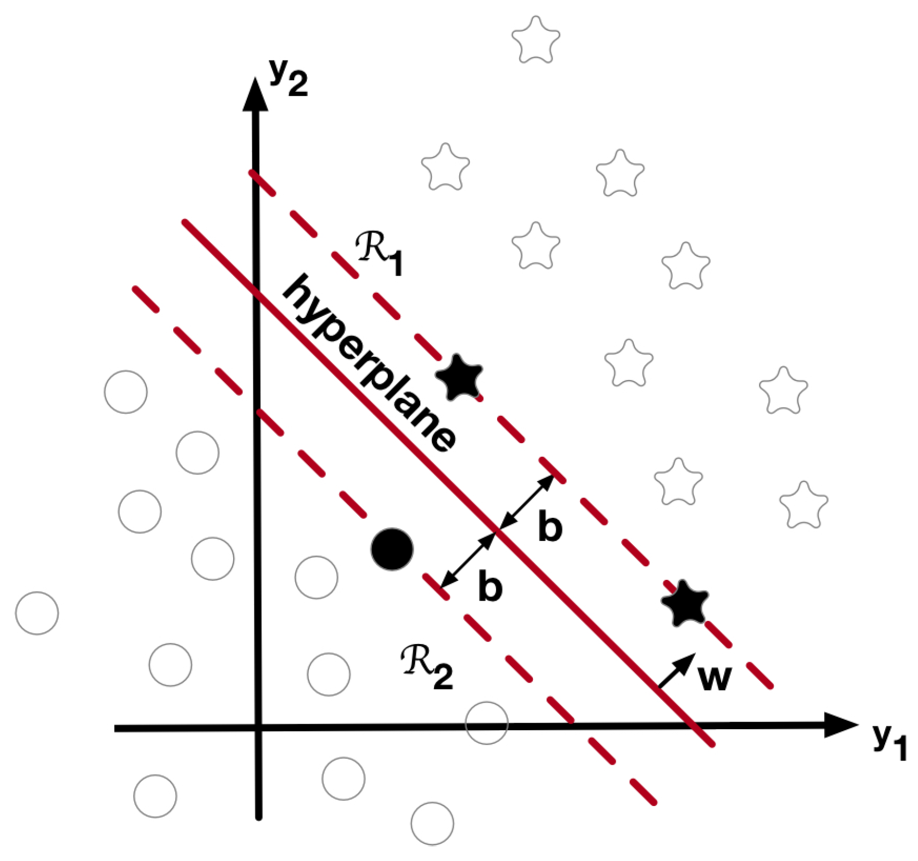
4.3.2. Support Vector Machines

This is a non-probabilistic classifier. The support vector machines (SVM) are based on the linear training machines with margins [57,58]. The linear discriminant function has the general form

$$g\left(\mathbf{x}\right)={\mathbf{w}}^T\mathbf{x}+w_0,$$

(10)

where $\mathbf{w}$ is a weight vector, and $w_0$ is the bias or threshold weight.

In the SVM methodology, each pattern ${\mathbf{x}}_j=[S_F,S_{CNN}]$ is transformed by

$${\mathbf{y}}_j=\phi \left({\mathbf{x}}_j\right),$$

(11)

where $j=1,2,\dots ,N$. With an appropriate nonlinear mapping $\phi$, the data can always be separated by a hyperspace, Figure 6. For each of these N patterns, let be $z_j=\pm 1$. A linear discriminant in an augmented $\mathbf{y}$ space is given by

$$g\left(\mathbf{y}\right)={\mathbf{a}}^T\mathbf{y},$$

(12)

where both the weight vector and the transformed pattern vector are augmented (compares it with Equation (10)). The first step to train an SVM is to choose the nonlinear function $\phi$. The goal is to minimize the magnitude of the weight vector. The problem was rewritten as maximizing the distance of the hyperplane by the Kuhn–Tucker construction,

$$\begin{array}{ccc}\hfill \mathcal{L}\left(\alpha \right)& =& \sum _{i=1}^M{\alpha }_i-\frac{1}{2}\sum _{i=1}^M\sum _{j=1}^M{\alpha }_i{\alpha }_j{z}_i{z}_j{\mathbf{y}}_i^T{\mathbf{y}}_j,\hfill \end{array}$$

(13)

$$\begin{array}{ccc}\hfill \sum _{i=1}^M{\alpha }_i{z}_i& =& 0,{\alpha }_i\ge 0.\hfill \end{array}$$

(14)

Let $\mathbf{K}$ a $M\times M$ matrix with elements

$$K(i,j)={\mathbf{y}}_i^T{\mathbf{y}}_j={\mathbf{y}}_i,{\mathbf{y}}_j=\phi \left({\mathbf{x}}_i\right),\phi \left({\mathbf{x}}_j\right),$$

(15)

using Equation (11). In Equation (13) is not required to know the mapping $\phi \left({\mathbf{x}}_i\right)$, it is enough to know the associated kernel $K(i,j)$. Two of the most common kernels are the linear kernel (SVM-L)

$$K(i,j)={\mathbf{y}}_i^T{\mathbf{y}}_j,$$

(16)

and the Gaussian kernel (SVM-G)

$$K(i,j)=e^{-\frac{\left|\right|{\mathbf{y}}_i-{\mathbf{y}}_j{\left|\right|}^2}{2{\sigma }^2}},$$

(17)

where $\sigma$ is the standard deviation.

4.4. The Ensemble Classifier

Pattern recognition methodologies perform efficiently with databases with balanced classes. Today, many of the applications, particularly medical ones, have unbalanced distribution. That causes the classifier to skew towards the majority class. Working with databases with unbalanced classes is one of the significant challenges for developing computer-aided diagnosis tools. One of the commonly used techniques to rebalance classes’ distribution is resampling techniques such as subsampling, oversampling, or a hybrid. However, the case of deleting relevant information could be presented. Or, in the other case, we are adding information by using synthetic data. Recently, it has been utilizing the assembly of multiple classifiers for working with unbalanced classes [59,60,61,62,63,64,65]. In this proposal, we use the ensemble of three classifiers with a linear plurality vote. The skin lesion image will be classified as one of the eight classes if two or three of the classifier spaces predict that it belongs to that class. Figure 7 shows a block diagram of the proposed computer-aided diagnosis methodology.

5. The Database

The computer-aided diagnosis proposed methodology was tested with the International Skin Imaging Collaboration (ISIC) 2019 dataset [66,67]. This dataset consisted of high-quality skin lesion color images of different sizes. The dataset comprised 25,331 images in eight different classes, including identification labels of the lesions and metadata associated with these lesions, such as age, anatomical site, and sex of the patient. The lesion classes are actinic keratosis (AK), basal cell carcinoma (BCC), squamous cell carcinoma (SCC), benign keratosis (BKL), melanoma (MEL), melanocytic nevus (NEV), dermatofibroma (DER), and the vascular lesion (VASC).

Table 1. International Skin Imaging Collaboration (ISIC) archive-2019, number of images per skin lesion classes.

Class Name	Class Abbrevation	Number of Images
actinic keratosis	AK	867
basal cell carcinoma	BCC	3323
squamous cell carcinoma	SCC	628
benign keratosis	BKL	2624
melanoma	MEL	4522
melanocytic nevus	NEV	$12,875$
dermatofibroma	DER	239
vascular lesion	VASC	253
Total		25,331

shows the distribution of images per class in the dataset.

6. Evaluation Metrics

The computer-aided diagnosis results had four possibilities: true positive classification, indicated by $TP$; false positive classification, marked as $FP$; false negative classification, showed like $FN$; and true negative classification, pointed out by $TN$. Based on these values, the four measures used to test the methodology robustness were

$$\begin{array}{ccc}\hfill accuracy& =& \frac{TP+TN}{TP+TN+FP+FN}\times 100\%,\hfill \end{array}$$

(18)

$$\begin{array}{ccc}\hfill precision& =& \frac{TP}{TP+FP}\times 100\%,\hfill \end{array}$$

(19)

$$\begin{array}{ccc}\hfill sensitivity& =& \frac{TP}{TP+FN}\times 100\%,\hfill \end{array}$$

(20)

$$\begin{array}{ccc}\hfill specificity& =& \frac{TN}{TN+FP}\times 100\%.\hfill \end{array}$$

(21)

The accuracy was the proportion of the total cases classified correctly as positive and negative $TP+TN$ between all possibilities presented $(TP+TN+FP+FN)$; this was a measure of bias. The precision was the conditional probability that measures the correct classifications $TP$ between the number of classifications indicated as positive $TP+FP$; this was a measure of the spread. The sensitivity or recall was the conditional probability that measures the proportion of the correct classification ($TP$) between all cases that should have been classified as correct ($TP+FN$). The specificity was the conditional probability that measured the proportion of true negative classification ($TN$) between the number of total cases who were rightly negative ($TN+FP$) [53].

7. Results

The proposed methodology was implemented in MatLab 2019b on an HP computer, Intel Core i5, 12 GB RAM. A total of four experiments were done. The ISIC archive-2019 had a significant imbalance between the majority and minority classes. To handle imbalanced classes, we used the ensemble method using three classifiers with a linear plurality vote. In Exp-1 and Exp-2, the performance metrics reported were for the dataset without splitting. In Exp-3 and Exp-4, the dataset was randomly sampled five times with replacement in 70% for the training part and 30% for the test. Since the original set was sampled with replacement, some elements were repeated in the training sets, and others were not presented. With the five sets, we trained the classifiers, and thus we obtained different predictions that helped us have a fair classification of the images. In the first experiment (Exp-1), the complete dataset was used, the 25,331 dermoscopy color-images of the ISIC archive-2019. The $\alpha$ parameter in the fractal signature was varied from $\alpha =-2$ to 2 with stride 0.1. The best performance was obtained with $\alpha =-2.0$.

Table 2. Confusion matrix of the Exp-1 with $\alpha =-2.0$. The dataset has 25,331 images.

	Training Dataset
	AK	BCC	SCC	BKL	MEL	NEV	DER	VASC
	867	3323	628	2624	4522	12,875	239	253
AK	662	91	3	16	5	90	0	0
BCC	22	3203	0	13	14	70	1	0
SCC	34	224	276	11	2	81	0	0
BKL	27	144	4	2105	39	305	0	0
MEL	37	111	5	85	3597	687	0	0
NEV	14	96	1	40	65	12,659	0	0
DER	3	54	3	10	14	108	47	0
VASC	3	33	3	5	10	105	0	94
Exp-1 response	802	3956	295	2285	3746	14,105	48	94

displays the confusion matrix output for the Exp-1 with $\alpha =-2.0$. The ISIC 2019 library had 867 AK, 3323 BCC, 628 SCC, 2624 BKL, 4522 MEL, 12875 NEV, 239 DER, 253 VASC. The computer-aided diagnosis response was 802 AK, 3956 BCC, 295 SCC, 2285 BKL, 3746 MEL, 14,105 NEV, 48 DER, 94 VASC. As was expected, the classes with an insufficient number of images were misclassified, like SCC, DER, and VASC. We must always keep in mind to have a representative dataset ${\mathbf{D}}_{\mathcal{C}}$ for the class $\mathcal{C}$ that allows us to reproduce or generate the space for that class. For ${\mathbf{D}}_{\mathcal{C}}$, all the images in $\mathcal{C}$ should be rewritten as a linear combination of the elements in ${\mathbf{D}}_{\mathcal{C}}$, which was not happening with the classes SCC, DER, and VASC. Based on the confusion matrix in Table 2, the true positive $TP$, false positive $FP$, false negative $FN$, and true negative $TN$ values were computed, as shown in

Table 3. Performance of the Exp-1 based on the confusion matrix in Table 2.

Class	Training Dataset	Exp-1 Response	TP	FP	FN	TN
AK	867	802	662	140	205	24,324
BCC	3323	3956	3203	753	120	21,255
SCC	628	295	276	19	352	24,684
BKL	2624	2285	2105	180	519	22,527
MEL	4522	3746	3597	149	925	20,660
NEV	12,875	14,105	12,659	1446	216	11,010
DER	239	48	47	1	192	25,091
VASC	253	94	94	0	159	25,078

. These values were used in Equations (18) to (21) to compute the performance of the computer-aided diagnosis of the Exp-1.

Table 4. The performance metrics obtained from the values in Table 3 for the Exp-1 with $\alpha =-2.0$.

Class	$\mathit{Accuracy}$ (%)	$\mathit{Precision}$ (%)	$\mathit{Sensitivity}$ (%)	$\mathit{Specificity}$ (%)
AK	98.64	82.54	76.36	99.43
BCC	96.55	80.97	96.39	96.58
SCC	98.54	93.56	43.95	99.92
BKL	97.24	92.12	80.22	99.21
MEL	95.76	96.02	79.54	99.28
NEV	93.44	89.75	98.32	88.39
DER	99.24	97.92	19.67	100.00
VASC	99.37	100.00	37.15	100.0
Mean ± SD	97.35 ± 2.04	91.61 ± 6.89	66.45 ± 29.09	97.85 ± 3.98

shows the percentage of the values per class of accuracy, precision, sensitivity, and specificity. As was expected, sensitivity was low due to poor representation of SCC, DER, and VASC images. The Exp-1 computer-aided diagnosis yielded a mean ± standard deviation for $accuracy=97.35\pm 2.04\%$, $precision=91.61\pm 6.89\%$, $sensitivity=66.45\pm 29.09\%$, and $specificity=97.85\pm 3.98\%$.

Experiment 2 (Exp-2) used a dataset of 24,839 images with 867 AK, 3323 BCC, 628 SCC, 2624 BKL, 4522 MEL, and 12,875 NEV. The 239 DER and 253 VASC images were not considered. Again, the $\alpha$ parameter in the fractal signature was varied from $\alpha =-2$ to 2 with stride 0.1. The best performance was obtained with $\alpha =-1.9$. For the Exp-2, the mean ± standard deviation of the computer-aided diagnosis was $accuracy=96.85\pm 1.71\%$, $precision=90.12\pm 6.07\%$, $sensitivity=79.25\pm 19.06\%$, and $specificity=97.42\pm 3.93\%$, as shown in

Table 5. The performance metrics obtained for Exp-2 with $\alpha =-1.9$. The dataset has 24,839 images.

Class	$\mathit{Accuracy}$ (%)	$\mathit{Precision}$ (%)	$\mathit{Sensitivity}$ (%)	$\mathit{Specificity}$ (%)
AK	98.62	82.68	76.47	99.42
BCC	96.78	82.63	96.21	96.88
SCC	98.55	94.98	45.22	99.94
BKL	97.22	92.78	79.88	99.27
MEL	95.73	96.53	79.39	99.27
NEV	94.16	91.12	98.31	89.69
Mean ± SD	96.85 ± 1.71	90.12 ± 6.07	79.25 ± 19.06	97.42 ± 3.93

. As is observed, when not considering the classes with very few images, the sensitivity increased, and the standard deviation decreased. So this confirmed the importance of having a good sampling for each of the classes.

For experiment 3 (Exp-3), the ISIC dataset of 25,331 dermoscopy color-images was randomly divided into 70% for the training dataset (17732 images) and 30% for the test dataset (7599 images). The $\alpha$ parameter in the fractal signature was varied from $\alpha =-2$ to 2 with stride 0.1. The best performance was obtained with $\alpha =0.4$. The mean of five realizations was reported in

Table 6. Mean ± SD of five performance metrics for the training dataset of the Exp-3 with $\alpha =0.4$. The training dataset has 17,732.

Class	$\mathit{Accuracy}$ (%)	$\mathit{Precision}$ (%)	$\mathit{Sensitivity}$ (%)	$\mathit{Specificity}$ (%)
AK	98.87 ± 0.07	85.78 ± 0.81	80.21 ± 1.80	99.54 ± 0.02
BCC	96.56 ± 0.13	81.00 ± 0.44	96.62 ± 0.29	96.55 ± 0.12
SCC	98.45 ± 0.05	92.94 ± 1.35	40.43 ± 2.05	99.92 ± 0.02
BKL	97.36 ± 0.07	92.92 ± 0.49	80.72 ± 0.65	99.29 ± 0.05
MEL	95.58 ± 0.10	95.54 ± 0.13	78.92 ± 0.60	99.20 ± 0.02
NEV	93.14 ± 0.08	89.34 ± 0.09	98.21 ± 0.12	87.91 ± 0.07
DER	99.16 ± 0.03	98.00 ± 2.75	10.87 ± 1.67	100.00 ± 0.00
VASC	99.33 ± 0.01	99.69 ± 0.70	29.16 ± 385	100.00 ± 0.00
Mean ± SD	97.31 ± 2.14	91.90 ± 6.28	64.39 ± 32.93	97.80 ± 4.15

. The Exp-3 for the training dataset gave the performance metric of $accuracy=97.31\pm 2.14\%$, $precision=91.90\pm 6.28\%$, $sensitivity=64.39\pm 32.93\%$, and $specificity=97.80\pm 4.15\%$. For the test dataset the computer-aided diagnosis got $accuracy=92.20\pm 6.74\%$, $precision=66.30\pm 23.46\%$, $sensitivity=38.43\pm 31.12\%$, and $specificity=93.60\pm 12.22\%$,

Table 7. Mean ± SD of five performance metrics for the test dataset of the Exp-3 with $\alpha =0.4$. The test dataset has 7599 images.

Class	$\mathit{Accuracy}$ (%)	$\mathit{Precision}$ (%)	$\mathit{Sensitivity}$ (%)	$\mathit{Specificity}$ (%)
AK	95.61 ± 0.26	38.81 ± 2.15	47.56 ± 2.79	97.33 ± 0.13
BCC	89.48 ± 0.28	57.72 ± 1.29	69.07 ± 0.63	92.51 ± 0.28
SCC	97.19 ± 0.13	34.48 ± 4.10	13.84 ± 1.19	99.32 ± 0.11
BKL	90.30 ± 0.21	55.55 ± 3.59	28.97 ± 1.90	97.34 ± 0.29
MEL	86.85 ± 0.18	81.83 ± 2.11	33.84 ± 0.59	98.37 ± 0.19
NEV	80.06 ± 0.55	73.36 ± 0.65	95.58 ± 0.39	63.95 ± 0.86
DER	99.07 ± 0.07	90.00 ± 22.36	3.08 ± 1.95	99.99 ± 0.01
VASC	99.06 ± 0.07	98.57 ± 3.14	15.49 ± 1.70	99.99 ± 0.01
Mean ± SD	92.20 ± 6.74	66.30 ± 23.46	38.43 ± 31.12	93.60 ± 12.22

. Finally, experiment 4 (Exp-4) did not consider the DER and VASC classes, and the dataset of 24,839 images was randomly divided into 70% for the training dataset (17387 images) and 30% for the test dataset (7452 images). The best performance was obtained with $\alpha =1.6$. Five realizations were executed for the training dataset obtaining an $accuracy=96.82\pm 1.85\%$, $precision=90.57\pm 5.19\%$, $sensitivity=79.35\pm 20.24\%$, and $specificity=97.39\pm 4.06\%$,

Table 8. Mean ± SD of five performance metrics for the training dataset of the Exp-4 with $\alpha =1.6$. The training dataset has 17,387 images.

Class	$\mathit{Accuracy}$ (%)	$\mathit{Precision}$ (%)	$\mathit{Sensitivity}$ (%)	$\mathit{Specificity}$ (%)
AK	98.87 ± 0.08	85.88 ± 1.56	80.52 ± 1.21	99.52 ± 0.07
BCC	96.83 ± 0.04	82.93 ± 0.14	96.29 ± 0.23	96.91 ± 0.05
SCC	98.48 ± 0.05	94.68 ± 1.86	41.87 ± 1.05	99.93 ± 0.02
BKL	97.28 ± 0.04	92.88 ± 0.28	80.55 ± 0.53	99.27 ± 0.03
MEL	95.55 ± 0.07	96.21 ± 0.30	78.69 ± 0.67	99.31 ± 0.06
NEV	93.92 ± 0.19	90.83 ± 0.29	98.14 ± 0.09	89.39 ± 0.37
Mean ± SD	96.82 ± 1.85	90.57 ± 5.19	79.35 ± 20.24	97.39 ± 4.06

. For the test dataset it had $accuracy=89.95\pm 6.05\%$, $precision=58.62\pm 17.54\%$, $sensitivity=47.89\pm 29.30\%$, and $specificity=91.60\pm 13.62\%$,

Table 9. Mean ± SD of five performance metrics for the test dataset of the Exp-4 with $\alpha =1.6$. The test dataset has 7452 images.

Class	$\mathit{Accuracy}$ (%)	$\mathit{Precision}$ (%)	$\mathit{Sensitivity}$ (%)	$\mathit{Specificity}$ (%)
AK	95.38 ± 0.30	38.25 ± 3.57	45.15 ± 1.91	97.26 ± 0.40
BCC	89.66 ± 0.21	59.15 ± 0.30	68.38 ± 0.83	92.87 ± 0.14
SCC	97.23 ± 0.23	40.12 ± 6.49	16.26 ± 3.14	99.36 ± 0.11
BKL	90.39 ± 0.16	58.13 ± 1.94	29.27 ± 0.80	97.53 ± 0.20
MEL	86.43 ± 0.28	81.66 ± 1.43	32.62 ± 1.15	98.37 ± 0.14
NEV	80.59 ± 0.45	74.40 ± 0.40	95.68 ± 0.28	64.17 ± 0.83
Mean ± SD	89.95 ± 6.05	58.62 ± 17.54	47.89 ± 29.30	91.60 ± 13.62

. As observed, in the performance of the training data metrics in Exp-4, when the classes with fewer images were eliminated, the $accuracy$, $precision$, and $specificity$ remained in the same range as Exp-3 but increases the $sensitivity$. Remember that the training methodologies in Exp-3 and Exp-4 did not see the images in the test database, the accuracy and specificity in both experiments showed excellent performance. However, the precision and sensitivity will need to be improved in the next stage of this work. There are several factors to consider that could affect the reliability of computer-aided diagnosis methodologies. The first thing to be analyzed is the stage of the extraction of characteristics, to determine if it is required to add more elements to the vector or if there are redundant elements. Afterwards, we must always keep in mind that we are working with unbalanced classes, which implies selecting how to handle them, using subsampling, oversampling, a hybrid between them or the assembly techniques, and the type of classifiers that are being used for the assembly.

8. Comparison with Other Methodologies

Garnavi et al. [33] developed a computer-aided diagnosis of melanoma detection. They used wavelet-decomposition and geometrical features of the lesion, and the classifiers SVM, random forest, logistic model tree, and naive Bayes. The dataset had 289 dermoscopy images: 114 malignant (M) and 175 benign (B) images, which were split by the training set with 40 M and 59 B images; validation set with 30 M and 57 B images; and, the test set with 44 M and 59 B images. They obtained an accuracy = 91.26%, and AUC = 0.937.

Barata et al. [34] built two computer-aided diagnoses of dermoscopy images for melanoma detection: one uses global features and the other local features. They employed the classifiers KNN, AdaBoost, SVM-RBF, bag of features (BoF). The dataset had 176 dermoscopy images: 25 MEL and 151 NEV images. To handle the classes’ unbalances, they repeated the melanoma features. The global method showed sensitivity = 96% and specificity = 80%. The local method presented sensitivity = 100% and specificity = 75%.

Shimizu et al. [40] used linear classifiers and a binary strategy. The dataset employed had 968 dermoscopy images. The detection rate reached was 90.48% for MEL, 82.51% for NEV, 82.61% for BCC, and 80.61% for seborrheic keratosis (SK). They employed 10-fold cross-validation to report the performance.

Wahba et al. [41] proposed a gray-level difference method in conjunction with the ABCD features. The dataset had 300 dermoscopy images per class of MEL, NEV, BCC, pigmented benign keratosis (PBK). Operating with the SVM classifier and five-fold cross-validation they reports an accuracy = 100%, sensitivity = 100%, specificity = 100%, precision = 100%.

Khan et al. [37] used the grey level co-occurrence matrix (GLCM), local binary pattern (LBP), and color features to produced a binary classifier. The data set had 146 MEL and 251 NEV digital images. The classifiers used were SVM, KNN, Naive Bayes, and decision trees. They reported accuracy = 96%, sensitivity = 97%, specificity = 96%, and precision = 97%.

Albahar [38] yielded a CNN to classify dermoscopy images of melanoma, nevus, seborrheic keratosis, squamous cell carcinoma, basal cell carcinoma, and lentigo. He divided the dataset into three equal parts of 8000 images of benign and malignant categories. A total of 5600 images pertained to the training set and 2400 for the validation set. He obtained AUC = 0.98, accuracy = 97.49%, specificity = 93.6%, and sensitivity = 94.3%.

Marka et al. [39] gave a review of the state-of-the-art in the automated detection of nonmelanoma skin cancer. They reported the computer-aided diagnoses for dermoscopy and non-dermoscopy images.

Wu et al. [42] trained five CNNs with SK, AK, rosacea (ROS), lupus erythematosus (LE), BCC, and SCC. They reported the best methodology results of 92.9%, 89.2%, and 84.3% recalls for the LE, BCC, and SK, respectively, and the mean recall and precision reached 77.0% and 70.8%. The training image set had: 1075 SK, 219 AK, 263 ROS, 1188 LE, 623 BCC, and 638 SCC. The test images set was composed of 52 SK, 58 AK, 55 ROS, 85 LE, 66 BCC, and 72 SCC. Different weights were used in the cost function to address the problem of data imbalance.

Gessert et al. [44] proposed an ensemble of deep learning models to classify the dermoscopy color-images in the ISIC archive-2019 challenge. The methodology worked with cropped and binarized images. In addition, to avoid the imbalance of the classes, they made data augmentation. Here was reported specificity of 72.5%, and when the metadata were also used, the specificity increased to 74.2%.

Bajwa et al. [45] presented a computer-assisted diagnosis of the set of four classifiers that reports the average of the predictions. They used DermNet and the ISIC-2018 file. For the training step, the images were cropping, horizontal flipping, and resizing (as required by neural networks, for example, the size of images must be 224 × 224 pixels or 331 × 331 pixels). They used stratified k-fold cross-validation with $k=5$. For the ISIC archive-2018 consisting of seven classes with a total of 23665 images, they obtained a weighted average for $precision=85.02\pm 09.10\%$, $sensitivity=80.46\pm 09.38\%$, $specificity=96.57\pm 07.15\%$ and $F1-Score=82.45\pm 08.38$ when classifying the 23,665 images.

9. Discussion

The diagnosis of a skin lesion by a dermatologist remains subjective. The diagnostic accuracy range is 64% to 80% [68,69,70,71], measured in specialized dermatology centers. Nowadays, most diagnoses are made by physician assistants, whose accuracy is lower than the dermatologist’s [72].

In this work, we proposed a computer-aided diagnosis to identify eight classes of skin lesions in dermoscopy color-images. The classes are actinic keratosis (AK), basal cell carcinoma (BCC), squamous cell carcinoma (SCC), benign keratosis (BKL), melanoma (MEL), melanocytic nevus (NEV), dermatofibroma (DER), and the vascular lesion (VASC). The methodology uses three fractal signatures, one signature per color in the RGB color-space. To handle the difference of the signatures’ lengths, we used the energy, variance, and entropy of the fractal signatures. These nine features concatenate with the 100 features obtained from the Densenet-201. We use three classifier spaces to construct an ensemble classifier based on the majority vote: the K-nearest neighbors (KNN) and the support vector machines (SVM) with linear and Gaussian kernels. The computer-aided diagnosis tested using 25,331 dermoscopy color-images from the ISIC archive-2019. Working with a hybrid methodology of three 1D fractal signatures and DenseNet-201 features allows us to strengthen the computer-aided diagnosis. We have more image information working with the fractal signatures since we do not have to reduce the image in size as required to work with a neural network. The computer-aided diagnosis presented excellent results like those obtained by the four ensembles CNNs by Gessert et al. [44] and Bajwa et al. [45]. A difference from the Gessert et al. and Bajwa et al. methodologies, in this proposal, we do not use artificial image generation or manipulation. Because there are various open-source alternatives for CNNs, the proposed methodology does not require computer equipment with high performance. That makes it viable to reproduce the same results with different programming languages on various platforms. However, we need to notice that CNNs are based on the convolution operation of the image with different filters, which require a large number of training images to extract all the possible ways that the image can be presented. That yields a high computational cost. Furthermore, to properly segment images with low-contrast edges and hair artifacts, such as those of skin lesions, specialized neural networks are required on the topic [8]. Due to these aspects, a viable option to reduce computational cost has been developing, using hybrid methodologies of CNNs with handcrafted feature extraction approaches, like this proposal.

10. Conclusions

We proposed a computer-aided diagnosis methodology for eight classes of dermoscopy color-digital images in the ISIC archive-2019. The classes are actinic keratosis, basal cell carcinoma, squamous cell carcinoma, benign keratosis, melanoma, melanocytic nevus, dermatofibroma, and vascular lesion. The methodology utilized 1D fractal features and Densenet-201 CNN features. In this work, a hybrid proposal between a convolutional neural network and a handcrafted feature extraction methodology was chosen to take advantage of both of these techniques. The aim is to reduce the operational computational cost of using various neural networks. It is well known that a neural network requires a vast training database to pursue an excellent performance since it is based on image convolution with several filters. The reason for such operational computational cost is that the convolution operation is not invariant to geometric transformations such as scale, rotation, and translation. The computer-aided diagnosis presented an average accuracy of 97.35%, an average precision of 91.61%, an average sensitivity of 66.45%, and an average specificity of 97.85%. As the diagnosis depends on the clinical experience of the human vision, the computer-aided diagnosis aims to be a tool to help them to eliminate the subjectivity as much as possible.

References

1. Fitzpatrick, B.T. The validity and practicality of sun-reactive skin types I through VI. Arch. Dermatol. 1988, 124, 869–871. [Google Scholar] [CrossRef] [PubMed]
2. Department of Health. National Skin Cancer Prevention Plan 2019–2022. Available online: https://www.gov.ie/en/publication/4655d6-national-skin-cancer-prevention-plan-2019-2022/ (accessed on 27 May 2019).
3. American Cancer Society. Skin Cancer. Available online: https://www.cancer.org/cancer/skin-cancer.html (accessed on 27 May 2019).
4. Hay, R.J.; Johns, N.E.; Williams, H.C.; Bolliger, I.W.; Dellavalle, R.P.; Margolis, D.J.; Marks, R.; Naldi, L.; Weinstock, M.A.; Wulf, S.K.; et al. The Global burden of skin disease in 2010: An analysis of the prevalence and impact of skin conditions. J. Investig. Dermatol. 2014, 134, 1527–1534. [Google Scholar] [CrossRef] [PubMed] [Green Version]
5. Castillo, D.A.; Bonilla-Hernández, J.D.; Castillo, D.E.; Carrasquilla-Sotomayor, M.; Alvis-Zakzuk, N.J. Characterization of skin cancer in a dermatologic center in Colombia. J. Am. Acad. Dermatol. 2018, 79, AB70. [Google Scholar]
6. Nachbar, F.; Stolz, W.; Merkle, T.; Cognetta, A.B.; Vogt, T.L.; Thaler, M.; Bilek, P.; Braun-Falco, O.; Plewig, G. The ABCD rule of dermatoscopy: High prospective value in the diagnosis of doubtful melanocytic skin lesions. J. Am. Acad. Dermatol. 1994, 30, 551–559. [Google Scholar] [CrossRef] [Green Version]
7. Folland, G.B. Fourier Analysis and Its Applications; American Mathematical Society: Providence, RI, USA, 2000; pp. 314–318. [Google Scholar]
8. Al-masni, M.A.; Al-antari, M.A.; Choi, M.T.; Han, S.M.; Kim, T.S. Skin lesion segmentation in dermoscopy images via deep full resolution convolutional networks. Comput. Meth. Prog. Biomed. 2018, 162, 221–231. [Google Scholar] [CrossRef]
9. Haralick, R.M.; Shanmugam, K.; Dinstein, I. Textural Features for Image Classification. IEEE Trans. Syst. Man Cybern. 1973, SMC-3, 610–621. [Google Scholar] [CrossRef] [Green Version]
10. Galloway, M.M. Texture analysis using gray level run lengths. Comput. Graph. Image Process. 1975, 4, 172–179. [Google Scholar] [CrossRef]
11. Haralick, R.M. Statistical and Structural Approaches to Texture. Proc. IEEE 1979, 67, 786–804. [Google Scholar] [CrossRef]
12. Sun, C.; Wee, W.G. Neighboring gray level dependence matrix for texture classification. Comput. Vis. Graph. Image Process. 1983, 23, 341–352. [Google Scholar] [CrossRef]
13. Amadasun, M.; King, R. Textural features corresponding to textural properties. IEEE Trans. Syst. Man Cybern. 1989, 19, 1264–1274. [Google Scholar] [CrossRef]
14. Chu, A.; Sehgal, C.; Greenleaf, J. Use of gray value distribution of run lengths for texture analysis. Pattern Recognit. Lett. 1990, 11, 415–419. [Google Scholar] [CrossRef]
15. Dasarathy, B.V.; Holder, E.B. Image characterizations based on joint gray level-run length distributions. Pattern Recognit. Lett. 1991, 12, 497–502. [Google Scholar] [CrossRef]
16. Ojala, T.; Pietikäinen, M.; Harwood, D. A comparative study of texture measures with classification based on featured distributions. Pattern Recognit. 1996, 29, 51–59. [Google Scholar] [CrossRef]
17. Tang, X. Texture Information in run-length matrices. IEEE Trans. Image Process. 1998, 7, 1602–1609. [Google Scholar] [CrossRef] [Green Version]
18. Guo, Z.; Wang, X.; Zhou, J.; You, J. Robust texture image representation by scale selective local binary patterns. IEEE Trans. Image Process. 2016, 25, 687–699. [Google Scholar] [CrossRef]
19. Liu, L.; Lao, S.; Fieguth, P.W.; Guo, Y.; Wang, X.; Pietikäinen, M. Median Robust Extended Local Binary Pattern for Texture Classification. IEEE Trans. Image Process. 2016, 25, 1368–1381. [Google Scholar] [CrossRef]
20. Dash, S.; Senapati, M.R. Gray level run length matrix based on various illumination normalization techniques for texture classification. Evol. Intell. 2018, 1–10. [Google Scholar] [CrossRef]
21. Al-antari, M.A.; Al-Masni, M.A.; Park, S.; Park, J.; Metwally, M.K.; Kadah, Y.M.; Han, S.M.; Kim, T.S. An Automatic Computer-Aided Diagnosis System for Breast Cancer in Digital Mammograms via Deep Belief Network. J. Med. Biol. Eng. 2018, 38, 443–456. [Google Scholar] [CrossRef]
22. Al-antari, M.A.; Han, S.M.; Kim, T.S. Evaluation of deep learning detection and classification towards computer-aided diagnosis of breast lesions in digital X-ray mammograms. Comput. Meth. Prog. Biomed. 2020, 196, 105584. [Google Scholar] [CrossRef]
23. Arivazhagan, S.; Ganesan, L.; Priyal, S.P. Texture classification using Gabor wavelets based rotation invariant features. Pattern Recognit. Lett. 2006, 27, 1976–1982. [Google Scholar] [CrossRef]
24. Regniers, O.; Bombrun, L.; Lafon, V.; Germain, C. Supervised Classification of Very High Resolution Optical Images Using Wavelet-Based Textural Features. IEEE Trans. Geosci. Remote Sens. 2016, 54, 3722–3735. [Google Scholar] [CrossRef] [Green Version]
25. Guerra-Rosas, E.; Álvarez-Borrego, J. Methodology for diagnosis of skin cancer on images of dermatologic spots by spectral analysis. Biomed. Opt. Express 2015, 10, 3876–3891. [Google Scholar] [CrossRef] [PubMed]
26. Depeursinge, A.; Püspöki, Z.; Ward, J.P.; Unser, M. Steerable wavelet machines (SWM): Learning moving frames for texture classification. IEEE Trans. Image Process. 2017, 26, 1626–1636. [Google Scholar] [CrossRef] [PubMed] [Green Version]
27. Guerra-Rosas, E.; Álvarez-Borrego, J.; Angulo-Molina, A. Identification of melanoma cells: A method based in mean variance of signatures via spectral densities. Biomed. Opt. Express 2017, 4, 2185–2194. [Google Scholar] [CrossRef]
28. Pardo, A.; Gutiérrez-Gutiérrez, J.A.; Lihacova, I.; López-Higuera, J.M.; Conde, O.M. On the spectral signature of melanoma: A non-parametric classification framework for cancer detection in hyperspectral imaging of melanocytic lesions. Biomed. Opt. Express 2018, 12, 6283–6301. [Google Scholar] [CrossRef] [Green Version]
29. Emerson, C.W.; Lam, N.S.N.; Quattrochi, D.A. Multi-scale fractal analysis of image texture and pattern. Photogramm. Eng. Remote Sens. 1999, 65, 51–61. [Google Scholar]
30. Lam, N.S.N.; Qiu, H.L.; Quattrochi, D.A.; Emerson, C.W. An Evaluation of Fractal Methods for Characterizing Image Complexity. Cartogr. Geogr. Inf. Sci. 2002, 29, 25–35. [Google Scholar] [CrossRef]
31. Chen, X.W.; Zeng, X.; van Alphen, D. Multi-class feature selection for texture classification. Pattern Recogn. Lett. 2006, 27, 1685–1691. [Google Scholar] [CrossRef]
32. Ashour, M.W.; Khalid, F.; Halin, A.B.; Darwish, S.H. Multi-class support vector machines for texture classification using gray-level histogram and edge detection features. IJAECS 2016, 3, 1–5. [Google Scholar]
33. Garnavi, R.; Aldeen, M.; Bailey, J. Computer-aided diganosis of Melanoma using border- and wavelet-based texture analysis. IEEE Trans. Inf. Technol. Biomed. 2012, 16, 1239–1252. [Google Scholar] [CrossRef]
34. Barata, C.; Ruela, M.; Francisco, M.; Mendoza, T.; Marques, J.S. Two systems for the detection of melanomas in dermoscopy images using texture and color features. IEEE Syst. J. 2014, 8, 965–979. [Google Scholar] [CrossRef]
35. Amelard, R.; Glaister, J.; Wong, A.; Clausi, D. High-level intuitive Features (HLIFs) for intuitive skin lesion description. IEEE Trans. Biomed. Eng. 2015, 62, 820–831. [Google Scholar] [CrossRef] [PubMed]
36. Spyridonos, P.; Gaitanis, G.; Likas, A.; Bassukas, I. Automatic discrimination of actinic keratoses from clinical photographs. Comput. Biol. Med. 2017, 88, 50–59. [Google Scholar] [CrossRef] [PubMed]
37. Khan, M.Q.; Hussain, A.; Rehman, S.U.; Khan, U.; Maqsood, M.; Mehmood, K.; Khan, M.A. Classification of melanoma and nevus in digital images for diagnosis of skin cancer. IEEE Access 2019, 7, 90132–90144. [Google Scholar] [CrossRef]
38. Albahar, M.A. Skin lesion classification using convolutional neural network with novel regularizer. IEEE Access 2019, 7, 38306–38313. [Google Scholar] [CrossRef]
39. Marka, A.; Carter, J.B.; Toto, E.; Hassanpour, S. Automated detection of nonmelanoma skin cancer using digital images: A systematic review. BMC Med. Imaging 2019, 19, 1–12. [Google Scholar] [CrossRef]
40. Shimizu, K.; Iyatomi, H.; Celebi, M.E.; Norton, K.A.; Tanaka, M. Four-class classification of skin lesions with task decomposition strategy. IEEE Trans. Biomed. Eng. 2015, 62, 274–283. [Google Scholar] [CrossRef]
41. Wahba, M.A.; Ashour, A.S.; Guo, Y.; Napoleon, S.A.; Abd-Elnaby, M.M. A novel cumulative level difference mean based GLDM and modified ABCD features ranked using eigenvector centrality approach for four skin lesion types classification. Comput. Meth. Prog. Biomed. 2018, 165, 163–174. [Google Scholar] [CrossRef]
42. Wu, Z.; Zhao, S.; Peng, Y.; He, X.; Zhao, X.; Huang, K.; Wu, X.; Fan, W.; Li, F.; Chen, M.; et al. Studies on different CNN algorithms for face skin disease classification based on clinical images. IEEE Access 2019, 7, 66505–66511. [Google Scholar] [CrossRef]
43. Garza-Flores, E.; Guerra-Rosas, E.; Álvarez-Borrego, J. Spectral indexes obtained by implementation of the fractional Fourier and Hermite transform for the diagnosis of malignant melanoma. Biomed. Opt. Express 2019, 10, 6043–6056. [Google Scholar] [CrossRef]
44. Gessert, N.; Nielsen, M.; Shaikh, M.; Werner, R.; Schlaefer, A. Skin lesion classification using ensembles of multi-resolution EfficientNets with meta data. MethodsX 2020, 1, 1008641-8. [Google Scholar] [CrossRef] [PubMed]
45. Bajwa, M.N.; Muta, K.; Malik, M.I.; Siddiqui, S.A.; Braun, S.A.; Homey, B.; Dengel, A.; Ahmed, S. Computer-aided diagnosis of skin diseases using deep neural networks. Appl. Sci. 2020, 10, 2488. [Google Scholar] [CrossRef] [Green Version]
46. Barnsley, M.F.; Devaney, R.L.; Mandelbrot, B.B.; Peitgen, H.O.; Saupe, D.; Voss, R.F. The Science of Fractal Images; Springer: New York, NY, USA, 1998; pp. 22–70. [Google Scholar]
47. Edgar, G. Measure, Topology, and Fractal Geometry, 2nd ed.; Springer: New York, NY, USA, 2000; pp. 165–224. [Google Scholar]
48. Backes, A.R.; Casanova, D.; Bruno, M.O. Plant leaf identification based on volumetric fractal dimension. Int. J. Pattern Recog. 2009, 23, 1145–1160. [Google Scholar] [CrossRef]
49. Florindo, J.B.; Bruno, O.M.; Landini, G. Morphological classification of odontogenic keratocyst using Bouligand-Minkowski fractal descriptors. Comput. Biol. Med. 2017, 81, 1–10. [Google Scholar] [CrossRef]
50. Florindo, J.B.; Bruno, O.M. Fractal Descriptors of Texture Images Based on the Triangular Prism Dimension. J. Math. Imaging Vis. 2019, 61, 140–159. [Google Scholar]
51. Silveira, M.; Nascimento, J.C.; Marques, J.S.; Marçal, A.R.S.; Mendonça, T.; Yamauchi, S.; Maeda, J.; Rozeira, J. Comparison of segmentation methods for melanoma diagnosis in dermoscopy images. IEEE J. Sel. Top. Signal Process. 2009, 3, 35–45. [Google Scholar] [CrossRef]
52. Celebi, M.E.; Wen, Q.; Iyatomi, H.; Shimizu, K.; Zhou, H.; Schaefer, G. Dermoscopy Image Analysis; Chapter A State-of-the-Art Survey on Lesion Border Detection in Dermoscopy Images; Celebi, M.E., Mendonca, T., Marques, J.S., Eds.; CRC Press: Boca Raton, FL, USA, 2015; pp. 97–129. [Google Scholar]
53. Deep, R. Probability and Statistics; Elsevier Academic Press: Cambridge, MA, USA, 2006; pp. 19–22, 104, 287. [Google Scholar]
54. Huang, G.; Liu, Z.; Van Der Maaten, L.; Weinberger, K. Densely Connected Convolutional Networks. In Proceedings of the IEEE Conference on Computer Vision and Pattern Recognition (CVPR), Honolulu, HI, USA, 21–26 July 2017; pp. 2261–2269. [Google Scholar]
55. Gonzalez, R.C.; Wood, R.E.; Eddins, S.L. Digital Image Processing with MATLAB; Tata McGraw-Hill: New Delhi, India, 2010; pp. 237–240, 253–259. [Google Scholar]
56. Bishop, C.M. Pattern Recognition and Machine Learning; Springer: New York, NY, USA, 2006; pp. 67–357. [Google Scholar]
57. Rogers, S.; Girolami, M. A First Course in Machine Learning; CRC Press: Boca Raton, FL, USA, 2011; pp. 169–205. [Google Scholar]
58. Duda, R.O.; Hart, P.E.; Stork, D.G. Pattern Classification, 2nd ed.; Wiley-Interscience: New York, NY, USA, 2001; pp. 20–513. [Google Scholar]
59. Galar, M.; Fernández, A.; Barrenechea, E.; Bustince, H.; Herrera, F. A review on ensembles for the class imbalance problem: Bagging-, boosting-, and hybrid-based approaches. IEEE Trans. Syst. Man Cybern. C 2012, 42, 463–484. [Google Scholar] [CrossRef]
60. Salunkhe, U.R.; Mali, S.N. Classifier ensemble design for imbalance data classification: A hybrid approach. Procedia Comput. Sci. 2016, 85, 725–732. [Google Scholar] [CrossRef] [Green Version]
61. Li, Y.; Guo, H.; Liu, X.; Li, Y.; Li, J. Adapted ensemble classification algorithm based on multiple classifier system and feature selection for classifying multi-class imbalanced data. Knowl.-Based Syst. 2016, 94, 88–104. [Google Scholar] [CrossRef]
62. Wang, Q.; Luo, Z.; Huang, J.; Feng, Y.; Liu, Z. A Novel Ensemble Method for Imbalanced Data Learning: Bagging of Extrapolation-SMOTE SVM. Comput. Intel. Neurosc. 2017, 2017, 1827016. [Google Scholar] [CrossRef]
63. Leon, F.; Floria, S.; Badica, C. Evaluating the effect of voting methods on ensemble-based classification. In Proceedings of the 2017 IEEE International Conference on INnovations in Intelligent SysTems and Applications (INISTA), Gdynia, Poland, 3–5 July 2017; pp. 1–6. [Google Scholar]
64. Wang, H.; Shen, Y.; Wang, S.; Xiao, T.; Deng, L.; Wang, X.; Zhao, X. Ensemble of 3D densely connected convolutional network for diagnosis of mild cognitive imparient and Alzheimer’s disease. Neurocomputing 2019, 333, 145–156. [Google Scholar] [CrossRef]
65. Mahbod, A.; Schaefer, G.; Wang, C.; Dorffner, G.; Ecker, R.; Ellinger, I. Transfer learning using a multi-scale and multi-network ensemble for skin lesion classification. Comput. Meth. Prog. Biomed. 2020, 193, 105475. [Google Scholar] [CrossRef] [PubMed]
66. Tschandl, P.; Rosendahl, C.; Kittler, H. Data Descriptor: The HAM10000 dataset, a large collection of multi-source dermatoscopic images of common pigmented skin lesions. Sci. Data 2018, 5, 180161. [Google Scholar] [CrossRef] [PubMed]
67. Codella, N.; Gutman, D.; Celebi, M.E.; Helba, B.; Marchetti, M.; Dusza, S.; Kalloo, A.; Liopyris, K.; Mishra, N.; Kittler, H.; et al. Skin lesion analysis toward melanoma detection: A challenge at the 2017 International Symposium on Biomedical Imaging (ISBI), hosted by the International Skin Imaging Collaboration (ISIC). In Proceedings of the IEEE 15th International Symposium on Biomedical Imaging (ISBI 2018), Washington, DC, USA, 4–7 April 2018; pp. 168–172. [Google Scholar]
68. MacKenzie-Wood, A.R.; Milton, G.W.; Launey, J.W. Melanoma: Accuracy of clinical diagnosis. Australas. J. Dermat. 1998, 39, 31–33. [Google Scholar] [CrossRef] [PubMed]
69. Miller, M.; Ackerman, A.B. How accurate are dermatologists in the diagnosis of melanoma? Degree of accuracy and implications. Arch. Dermatol. 1992, 128, 559–560. [Google Scholar] [CrossRef]
70. Lindelöf, B.; Hedblad, M.A. Accuracy in the clinical diagnosis and pattern of malignant melanoma at a dermatological clinic. J. Dermatol. 1994, 21, 461–464. [Google Scholar] [CrossRef]
71. Grin, C.M.; Kopf, A.W.; Welkovich, B.; Bart, R.S.; Levenstein, M.J. Accuracy in the clinical diagnosis of malignant melanoma. Arch. Dermatol. 1990, 126, 763–766. [Google Scholar] [CrossRef]
72. Anderson, A.M.; Matsumoto, M.; Saul, M.I.; Secrest, A.M.; Ferris, L.K. Accuracy of skin cancer diagnosis by physician assistants compared with dermatologists in a large health care system. JAMA Dermatol. 2018, 154, 569–573. [Google Scholar] [CrossRef] [Green Version]
Figure 1. Triangular prism.
Applsci 10 05954 g001
Figure 2. Fractal signature examples. (a) Color image of actinic keratosis. (b) F R , F G , F B fractal signatures from channel red, green, and blue, respectively. (c) Amplification region of the signatures’ graphs to see the difference in the values of the three signatures.
Applsci 10 05954 g002
Figure 3. DenseNet architecture. (a) Block diagram of the concatenation operation, indicated by a C within a yellow circle. (b) Block diagram of the forward propagation. (c) Block diagram of the layer composition.
Applsci 10 05954 g003
Figure 4. Block diagram of a deep DenseNet. The C within a yellow circle represents the concatenation operation.
Applsci 10 05954 g004
Figure 5. Sketch of the K-NN classifier space using five neighbors. The red star represents the test point. The black stars, squares, and diamonds are the training points.
Applsci 10 05954 g005
Figure 6. Sketch of the linear machine with margins. The black star and black circles represent the support vectors.
Applsci 10 05954 g006
Figure 7. Block diagram of the proposed methodology. The C within a yellow circle represents the concatenation operation.
Applsci 10 05954 g007