Overview of Compressed Sensing: Sensing Model, Reconstruction Algorithm, and Its Applications

Abstract

With the development of intelligent networks such as the Internet of Things, network scales are becoming increasingly larger, and network environments increasingly complex, which brings a great challenge to network communication. The issues of energy-saving, transmission efficiency, and security were gradually highlighted. Compressed sensing (CS) helps to simultaneously solve those three problems in the communication of intelligent networks. In CS, fewer samples are required to reconstruct sparse or compressible signals, which breaks the restrict condition of a traditional Nyquist–Shannon sampling theorem. Here, we give an overview of recent CS studies, along the issues of sensing models, reconstruction algorithms, and their applications. First, we introduce several common sensing methods for CS, like sparse dictionary sensing, block-compressed sensing, and chaotic compressed sensing. We also present several state-of-the-art reconstruction algorithms of CS, including the convex optimization, greedy, and Bayesian algorithms. Lastly, we offer recommendation for broad CS applications, such as data compression, image processing, cryptography, and the reconstruction of complex networks. We discuss works related to CS technology and some CS essentials.

1. Introduction

With the expansion of some traditional networks and the advent of the Internet of Things in recent years, network structures are more complex, and transmitted data in the networks are bigger, as is shown in Figure 1. The numbers of smart sensors and connected devices continue to grow in many practical network applications. This is a huge challenge for network communication, such as with regard to transmission efficiency and network security. Compressed sensing (CS) emerged, which is able to satisfy the needs of transmission efficiency and security at the same time.

Compressed sensing is an advanced method of acquiring and processing signals, and it was first proposed by Donoho [1,2]. It can accurately recover the original signal from a few incoherent measurements. In CS, fewer samples are required to reconstruct sparse or compressible signals, which breaks through the traditional Nyquist–Shannon sampling theorem. Suppose that x is a discrete signal, which is transformed into matrix y by a matrix $\Phi$ with $M\times N$ dimensions. The CS process can be expressed as

$$y=\Phi x,$$

(1)

where $M<N$, $y\in R^M$, and $\Phi$ is the sensing or measurement matrix. From Equation (1), signal x with $N\times N$-dimension is compressed into signal y with $M\times N$ dimensions. x is unsolvable by y from Equation (1) because the number of equations is less than that of the unknowns. The precondition of solvability for x is that x be sparse or that x be sparse on some orthogonal bases, that is,

$$x=\Psi s,$$

(2)

where $\Psi$ is an orthogonal matrix with $N\times N$ dimensions, which satisfies the conditions that $\Psi {\Psi }^T=I$ and ${\Psi }^T\Psi =I$. Here, $\Psi$ is the sparsity matrix, and s is a sparse vector. When K values of s are nonzero, and other $N-K$ values are zero ($K\ll N$), we call the vector s K-sparse. Common sparsity matrices are discrete Fourier transform (DFT) [3], discrete-wavelet-transform (DWT) [4], and discrete-cosine-transform (DCT) [5] matrices. As is shown in Figure 2, on the basis of Equations (1) and (2), we have

$$y=\Phi x=\Phi \Psi s=\Theta s,$$

(3)

where $\Phi \Psi$ is the sensing matrix. To construct x from y, sensing matrix $\Phi \Psi$ must be in accordance with the restricted isometry property (RIP) [6]. RIP is

$$1-{\delta }_k\le \frac{{∥\Theta v∥}_2}{{∥v∥}_2}\le 1+{\delta }_k,$$

(4)

where ${\delta }_k\in (0,1)$, v is an arbitrary sparsity signal. The process of reconstruction can be described as

$$\underset{\tilde{s}}{min}{∥\tilde{s}∥}_{l_1}s.t.y=\Theta \tilde{s},$$

(5)

which is a convex-optimization problem.

A large amount of work has been done on CS theory and applications [7,8]. Based on the CS introduction above, CS is principally composed of two important parts, sensing and reconstruction. In the sensing part, we use a sensing matrix that satisfies certain conditions to obtain a sparse signal. There are many classical sensing matrices, such as the random, deterministic, and structured random matrices. The Gaussian and Bernoulli matrices are typical random matrices. Common deterministic matrices are the polynomial and chaotic matrices. The Toeplitz and the Hadamard matrices are structured random matrices. In the reconstruction step, we use a measurement vector and CS algorithms to reconstruct the original signal. There are many kinds of reconstruction CS algorithms, such as the convex-optimization, greedy, and Bayesian algorithms. In addition to theoretical research, CS has also been utilized in many different domains such as data compression, image encryption, and cryptography.

This paper is divided into five sections. Section 2 introduces several common CS methods, including sparse dictionary, block CS, chaotic CS, deep-learning CS, and semitensor-product CS. Section 3 provides CS reconstruction algorithms like the convex-optimization, greedy, Bayesian, and noniterative-reconstruction algorithms. Section 4 briefly presents compressed-sensing applications. Lastly, conclusions are presented in Section 5.

2. Sensing Methods

Sensing methods have always been a hotspot in CS research. The sensing process also affects signal sampling and the accuracy of signal reconstruction. The main operation of a sensing step is to correlate a sparse signal with a proper sensing matrix without any prerequisites. In this section, we briefly introduce several sensing methods.

2.1. Sparse Dictionary Sensing

An important topic for sparse-representation research is signal sparse representation under a redundant dictionary. The current sparse representation of signals under redundant dictionaries focuses on the construction of sparse dictionaries, and the design of fast and efficient sparse-decomposition methods. Conventionally, sparsifying dictionary learning aims to construct a proper dictionary $\Psi$ and a matrix s to minimize sparse-representation errors. On the basis of Equation (2), the sparse-representation error is defined as follows:

$$E\triangleq x-{\Psi ssubjectto\Vert s(:,k)\Vert }_0\le K,\forall k,$$

(6)

where K is the sparsity of s. In the design of CS systems, besides dictionary $\Psi$, another important aspect is to choose a suitable sensing matrix $\Phi$ that can accurately construct original signal x by measurement y. $\Theta =\Psi \Phi$ in Equation (3) shows that the sparsity of measurement y is also an important aspect influencing the reconstruction accuracy of x.

Bai et al. embedded a sensing matrix into the problem of sparse dictionary learning, and proposed an alternative optimization strategy [9]. Previously, Duarte-Carvajalino et al. had proposed a similar framework [10]. In [9], Bai et al. optimized the problem of sparse dictionary learning by embedding a measurement matrix. The optimization process is as follows:

$$\left\{\begin{array}{c}mi{n}_{\Phi ,\Psi ,s}{\Vert A-B\Psi s\Vert }_F^2\triangleq ϝ(\Phi ,\Psi ,s)\hfill \\ {\Vert s(:,k)\Vert }_0\le K,\forall k,\Phi =f(\Psi )\hfill \end{array}\right.,$$

(7)

where

$$A\triangleq {[\sqrt{1-\alpha }\Phi X,\sqrt{\alpha }X]}^T,B\triangleq {[\sqrt{1-\alpha }\Phi ,\sqrt{\alpha }{I}_N]}^T.$$

(8)

Both A and B are independent of s. Sensing matrix $\Phi$ was denoted as $\Phi =f(\Psi )$ because it was decided by a given sparsity matrix $\Psi$, which is also called dictionary $\Psi$. The authors further proposed an optimized measurement matrix and a new algorithm to solve the corresponding optimization problem.

Another novel dictionary-based approach was proposed and applied in diffusion-tensor imaging (DTI) [11]. It combined adaptive dictionaries and $T_2$-weighting correction to form a compressed-sensing framework to reconstruct undersampled DTI data. This method could improve spatial resolution, the flexibility of the diffusion protocol, and application feasibility.

2.2. Block-Compressed Sensing

Block-compressed sensing (BCS) completes data acquisition and compression by lightweight measurement. When dealing with high-dimensional images and videos, BCS is the most appropriate approach and it can utilize its biggest advantage. This method divides the image into many small patches, and operates on each image patch separately during measurement and reconstruction, which reduces computational complexity and greatly saves sensing-matrix storage space. In BCS, the measurement matrix is small, which is conducive to storage. The measurement value of each image patch can be independently sent after being obtained. The receiver can also independently reconstruct the image patch according to the data, and realize real-time performance. Consider an $I_r\times I_c$ image with a total of $N=I_r{I}_c$ pixels. We divided the image into sub-blocks with a size of $B\times B$, and sampled with the same sensing matrix. The vectorized signal of the i-th block is denoted as $x_i$. Corresponding output CS vector $y_i$ is

$$y_i={\Phi }_B{x}_i,$$

(9)

where ${\Phi }_B$ is an $n_B\times B^2$ matrix and $n_B=\lfloor \frac{n{B}^2}{N}\rfloor$. ${\Phi }_B$ can be an orthonormalized random matrix, i.e., Gaussian and Bernoulli matrices. Then, measurement matrix $\Phi$ in Equation (1) can be represented as follows:

$$\Phi =\left(\begin{array}{cc}{\Phi }_B& \\ & \ddots \\ & & {\Phi }_B\end{array}\right),$$

(10)

where $\Phi$ is a block diagonal matrix. From Equation (10), we can see that BCS is storage-saving, as it just requires to store an $n_B\times B^2$ matrix ${\Phi }_B$ rather than an $n\times N$ matrix.

Computational complexity and recovery performance are highlighted at both encoder and decoder. To solve the two problems above, Zhang et al. introduced and investigated the BCS strategy with matrix permutation that was used before sampling to reduce the maximal level of signal block sparseness [12]. The matrix-permutation procedure was as follows:

• Reshape 2D signal $X\in R^{\sqrt{N}\times \sqrt{N}}$ to a new 2D signal $X^{†}=[X_1,X_2,\cdots ,X_L]\in R^{\sqrt{n}\sqrt{NL}}$.
• We used an appropriate permutation matrix $P\in R^{\sqrt{NL}\times \sqrt{NL}}$ to process $X^{†}$, and the process procedure was as follows:

  $$X^{\ell }=X^{†}P,$$

  (11)

  where $X^{\ell }\in R^{\sqrt{n}\times \sqrt{NL}}$ is the permutated 2D sparse signal.

After the matrix-permutation procedure, the block-sampling process can be performed as follows:

$$y^{\ell }={\Phi }_B{x_i}^{\ell },$$

(12)

where ${x_i}^{\ell }\in R^n$ represents the vectorized signal of the i-th block of $X^{\ell }$, and ${y_i}^{\ell }\in R^m$ is the measurement vector of ${x_i}^{\ell }$. Compared with traditional BCS approaches, the matrix-permutation-based BCS method has an advantage in the peak signal-to-noise ratio (PSNR) of the recovery images.

On the basis of BCS, Bigot et al. presented a random-sampling approach that projected the signal onto blocks of measurement vectors [13]. There is a typical example when the block consists of horizontal lines in the two-dimensional Fourier plane. They theoretically proved the number of blocks that could be used to accurately reconstruct sparse signals. The matrices, constructed by stacking random measurement blocks, are significant in the application because they can be easily formed on many imaging devices.

Traditional BCS methods rely on independent block image acquisition and independent block reconstruction. In order to enforce smoothness across block borders in BCS, Coluccia et al. proposed a method that used partially overlapping blocks to modify the sensing and reconstruction process [14]. They computed a fast preview from the blocks, which imposed the similarity of block borders and was used as a predictor of the entire block.

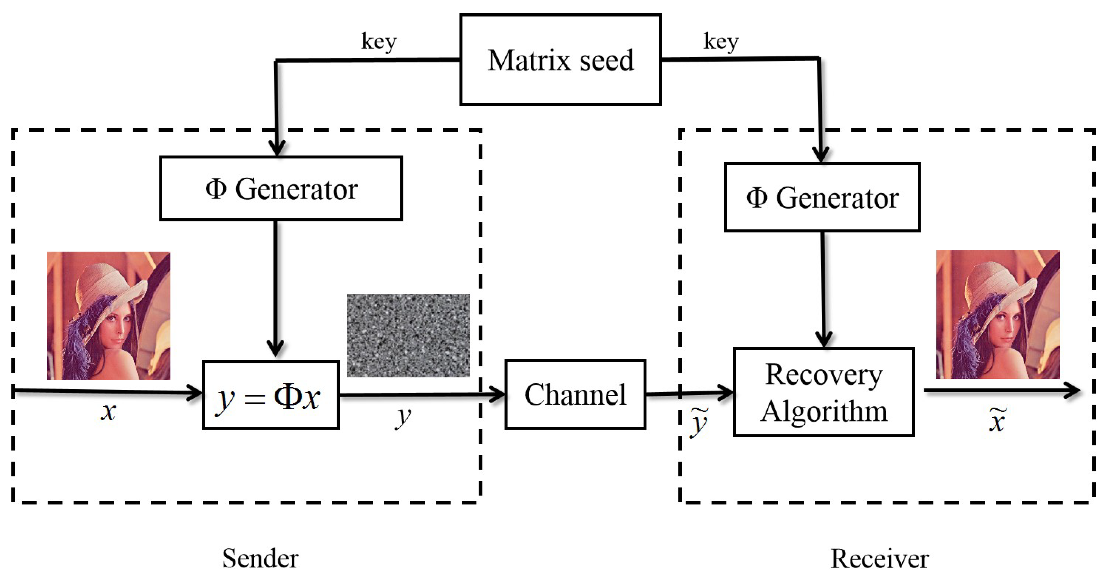
2.3. Chaotic Compressed Sensing

Since chaotic sequences generated by chaotic systems are pseudorandom, they are well-suited to be used as measurement matrices. In chaotic compressed sensing (CCS), chaotic systems can generate pseudorandom sequences by certain methods, which simplifies the construction of sensing matrices compared to a random-sensing matrix. We take the Chebyshev chaotic system as an example [15]:

$$z_{k+1}=cos(warccos{z}_k),$$

(13)

where $w\ge 2$, $z_k\in [-1,1]$. If parameter w and initiation value $z_0$ are given in advance, sequence $z_k$, $k=1,2,3...$, can then be generated on the basis of Equation (13). After obtaining this sequence, we use sampling distance d and sampling initial position $n_0$ to obtain the following sampled sequence:

$$x_n=z_{n_0+dn}.$$

(14)

In chaotic systems, the starting value and chaotic parameter have high sensitivity. A completely different sequence is obtained by slightly disturbing the starting value or system parameter, which proves that chaotic systems have high security.

Gan et al. proposed CCS by using the chaotic system of the T-way Bernoulli shift [16], and applied it to data transmission to achieve security. The CCS-based secure-data-transmission scheme has inherent encryption attributes with no additional cost. In this scheme, they used the Bernoulli chaotic system to generate the Bernoulli shift chaotic sequence, which constructs the Bernoulli chaotic-sensing matrix (BCsM).

To guarantee transmission security, Peng et al. improved the generation of chaotic measurement matrix, including chaotic parameters, sampling rate, matrix mapping functions, etc. [17]. We only need to save the matrix seeds such as the initial value, chaos parameters, sampling start position and sampling step, instead of saving the entire sensing matrix. The chaotic sensing matrix can be given as

$$\Phi =T\left(S(n_0,d,C(z_0,\epsilon ))\right)$$

(15)

where $z_0$, initial value; $\epsilon$, chaotic parameter; C, chaotic system; S, sampler; and T, mapping function. According to sampling initial position $n_0$ and sampling step d, the chaotic sequence was obtained after sampling. The required sensing matrix for chaotic compressed sensing could be generated with the mapping function. Compared with traditional CCS, the improved CCS simultaneously solves the problems of energy efficiency and security, and performs very well in image encryption.

Yao et al. presented the incoherence-rotated-chaotic (IRC) matrix as a measurement matrix [18]. They used the pseudorandomness character of chaotic sequences, the concepts of incoherent factors, and rotation to obtain the IRC sensing matrix. The obtained IRC sensing matrix was suitable for sparse reconstruction, satisfying the RIP criterion during the sparse-reconstruction phase and performing well in RIP with a smaller RIP ratio. Simulation results showed that the IRC matrix performed better than classical random-sensing matrices did.

2.4. Deep-Learning Compressed Sensing

The combination of deep learning and compressed sensing has attracted much attention. Adler et al. presented a deep-learning approach for block CS. They deployed a fully connected network to be performed on the block-based linear-perception and nonlinear-reconstruction section [19]. They employed a deep neural network that performed BCS by independently processing each block as per Equation (9). They proposed a fully connected network with four layers:

• input layer with $B^2$ nodes (B is block size);
• compressed-sensing layer, $B^{2}R$ nodes, $R\ll 1$ (its weights form the sensing matrix);
• $K\ge 1$ reconstruction layers, $B^{2}T$ nodes, each followed by a rectified linear unit (ReLU) [20] activation unit where $T>1$ is the redundancy factor; and
• output layer, $B^2$ nodes.

Compared with popular BCS methods such as block-compressed sensing smooth Landweber with dual-tree discrete wavelet transform (BCSSPL-DDWT) [21], multiscale block-compressed sensing smooth Landweber (MS-BCS-SPL) [22], and multihypothesis block-compressed sensing smooth Landweber (MH-BCS-SPL) [23], this method performed well with regard to recovery quality and calculation time.

Learning from convolutional networks, a deep-learning-based sparse-measurement matrix was presented to reduce the sampling calculation complexity and improve CS reconstruction quality [24]. The method had two subnetworks, the sample and reconstruction subnetworks. They assumed that block size $N_B$ in block CS was $B\times B$, and measurement size for every block was $N_b=\lfloor \frac{M}{N}{N}_B\rfloor$. The k-th line of sensing matrix $\Phi$ was denoted as

$$\Phi \left(k\right)=\{a_{k,1},a_{k,2},\cdots ,a_{k,N_B}\}.$$

(16)

The sparse degree is $ϝ(\Phi )=\frac{\nu }{N_b{N}_B}=\alpha (0\le \alpha <1)$, where $\nu$ is the number of nonzero elements in $\Phi$, and $N_b{N}_B$ is the whole elements in $\Phi$. To generate the target sample matrix, a sparsity constraint was added as follows:

$$S\left(a_{k,i}\right)=\left\{\begin{array}{c}0,\mid a_{k,i}\mid \le \mu \hfill \\ a_{k,i},\mid a_{k,i}\mid >\mu ,\hfill \end{array}\right.$$

(17)

where $k=1,2,\cdots ,N_b,i=1,1,\cdots ,N_B$, and $\mu$ is the $(1-\alpha )N_b{N}_B$-th smallest element in $\mid \Phi \mid$. $\Phi \left(k\right)$ is the k-th kernel of the convolutional layer in the sample subnetwork, and $a_{k,i}$ is the i-th value of this kernel. The normalization constraint for k-th kernel was formulated as

$$\Gamma \left(s_{k,j}\right)=\frac{s_{k,j}}{\sqrt{{\sum }_{i=1}^{N_B}{s_{k,j}}^2}},j=1,2,\cdots ,N_B,$$

(18)

where $s_{k,j}=S\left(a_{k,j}\right)$ and its derivative performed as

$$\Gamma {\left(s_{k,j}\right)}^{\prime }=\frac{\sqrt{\omega }-\frac{s_{k,j}^2}{\sqrt{\omega }}}{\sqrt{\omega }},\omega =\sum _{i=1}^{N_B}.{s_{k,i}}^2$$

(19)

On the basis of Equation (18), the normalized sampling matrix was obtained.

Sun et al. presented a deep-learning method for quantizing CS called BW-NQ-DNN [25]. The BW-NQ-DNN framework consists of three parts: a nonuniform quantizer, a binary sensing matrix, and a noniterative recovery solver. These three parts have joint optimization through BW-NQ-DNN training. BW-NQ-DNN not only saves a lot of storage and energy, but it also surpasses the most advanced CS-based approaches. When the compression ratio is very high, this method still performs well in recovery performance and classification accuracy.

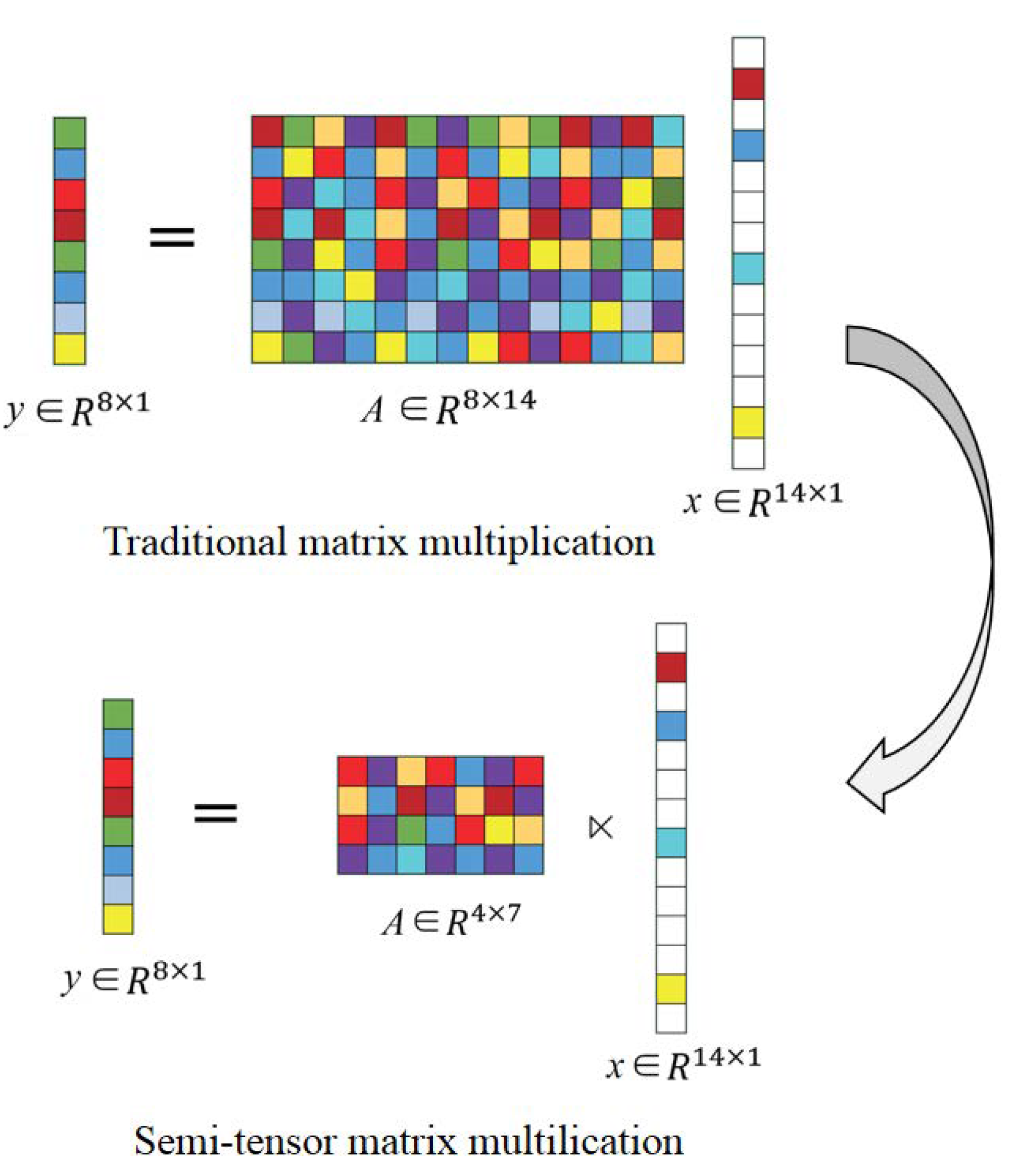
2.5. Semitensor-Product Compressed Sensing

Cheng et al. presented the semitensor product (STP) of matrices that broke through the limitation of conventional matrix operations. They further proposed an evolution of the traditional matrix product [26,27,28,29]. Traditional matrix multiplication should meet the limitations of matrix dimensions, that is, the column number of matrix A must equal the row number of matrix x, as is shown in Figure 3. STP theory breaks through this limitation, and it can execute matrix multiplication when the dimensions of two matrices are unmatched. Moreover, STP maintains the main properties of ordinary matrix multiplication.

Suppose that u is a row vector of dimension $np$, and v is a column vector of dimension p. By splitting u into p equal blocks, that is, $u^1,\cdots ,u^p$, each part $u^i$ is a row vector of dimension n. The definition of STP, represented by ⋉, is

$$u⋉v=\sum _{i=1}^p{u}^i{v}_i\in R^{1\times n}.$$

(20)

Similarly,

$$v^T⋉u^T=\sum _{i=1}^p{v}_i{\left(u^i\right)}^T\in R^{n\times 1}$$

Let $A\in R^{m\times n}$ and $B\in R^{p\times q}$. If either n is a factor of p or p is a factor of n, then we define the semitensor product of A and B as follows:

$$A⋉B=\left(\begin{array}{ccc}{A}_1⋉B^1& \cdots & A_1⋉B^q\\ ⋮& \ddots & ⋮\\ A_m⋉B^1& \cdots & A_m⋉B^q,\end{array}\right)$$

(21)

where $A_i$ is the i-th row of A, and $B^j$ is the j-th column of B. Equivalently, we can also define the STP of A and B by using the Kronecker product:

$$A⋉B=(A\otimes I_{t/n})(B\otimes I_{t/p}),$$

(22)

where t is the least common multiple of n and p, i.e., $t=lcm(n,p)$.

Xie et al. proposed semitensor-product compressed sensing (STP-CS), which combined semitensor product and compressed sensing [30]. They analyzed STP-CS from a theoretical perspective to demonstrate that the sparse solution is unique with regard to spark and coherence. The RIP criterion is satisfied in the STP-CS model. There are many classical sensing matrices that can be used in STP-CS, such as the Gaussian, Bernoulli, and chaotic matrices. These classical matrices can be used in STP-CS because the RIP configuration of order k in STP-CS is equivalent to that in conventional CS. On the basis of the semitensor product, STP-CS uses a low-dimensional sensing matrix to compress high-dimensional signals. The storage space needed in STP-CS is greatly saved compared with that in block-compressed sensing (BCS) with small block size. The semitensor product can be used to improve the reconstruction algorithm to realize parallel reconstruction, which can simultaneously perform signal reconstruction in multiple CS decoders, resulting in a reduction in total reconstruction time.

An application of STP-CS was presented to reduce calculation energy consumption, and it was applied to the communication of wireless sensor networks (WSNs) [31]. In terms of recovery quality, STP-CS is almost equal to conventional CS and CCS. Wang et al. proposed a random-sampling method based on the STP-CS framework [32]. They used an improved iteratively reweighted least-squares (IRLS) algorithm to obtain the values of the sparse vector. Simulation results showed that their method could save at least one-quarter of the storage resources when ensuring reconstruction performance.

The P-tensor product (PTP) was proposed on the basis of STP. It not only solved the dimensional-matching problem in matrix multiplication, but also provided a new method for angle calculation between different dimensional vectors [33]. For example, we can calculate the angle between a one- and a three-dimensional vector by PTP. PTP compensates for the limitations of STP when performing operations on vectors with different dimensions. In PTP, a smaller matrix is changed into a larger matrix, conforming to dimension matching by the tensor operation of matrix P. The choice of matrix P is not limited, and matrix P can be any kind of matrix. When PTP is combined with CS, the high-dimension signal can be measured by low-dimension sampling. Hence, storage space is significantly reduced.

2.6. Other Sensing Methods

Traditional compressed sensing associates sparse signals with a common sensing matrix regardless sparse domain. However, the performance of the sensing matrix is very problematic. Especially when the sensing matrix is a partial orthogonal sensing matrix, sensing fails because the signal is sparse in some transform domains. This problem is mainly because of the consistency of the sensing matrix with the sparsity matrix. Nouasria et al. proposed a robust sensing approach that multiplied the sensing matrix by the inverse matrix of the sparsity matrix in the sensing step [34]. The operation process of the random sensing matrix, especially the partial orthogonal sensing matrix, was improved.

So far, the sensing schemes of common CS theoretical models consist of random isolated measurements whose elements are randomly generated variables. Boyer et al. introduced the concept of measurement blocks [35]. In their scheme, the measurements of the sensing scheme were no longer a set of isolated measurements, but a set of measurements that might represent any shape (for example, parallel or radial lines).

Ishikawa et al. proposed another CS construction approach without randomness [36]. Their matrices had low incoherence. In order to obtain a CS matrix with low incoherence, an identity matrix with coherence 0 could be used as part of the CS matrix. In the meantime, they added vectors into their scheme under the basis of low coherence. Their CS matrix was given by the following:

$$A=\left[E\right|v_1,v_2,v_3,\cdots ,v_{n-m}],$$

(23)

where E, $m\times m$ identity matrix; $v_i$, m-dimensional appended vector with low coherence; and the dimension of A was $m\times n$, where $m\ll n$. Compared to existing random matrices, the matrix constructed by this approach could achieve higher recovery accuracy. However, there were still two problems to be solved: failure in some cases and the compression-ratio increment.

3. Reconstruction Algorithm

A large number of works were done to study the recovery algorithm of compressed sensing. These studies focused on the stable construction, low calculation, and reconstructed accuracy of signals, especially with small measurements. This section introduces reconstruction algorithms such as the convex-optimization, greedy, and Bayesian algorithms.

3.1. Convex-Optimization Algorithm

The convex-optimization algorithm converts a nonconvex problem into a convex one to solve signal approximation. Suppose that $J\left(x\right)$ is the convex cost that promotes sparsity. That is to say, the value of $J\left(x\right)$ is small when signal x is in high sparsity. On the basis of Equation (5), the reconstruction of signal x without noise could be described as

$$min\left\{J\right(x\left)\right\},subjecttoy=\Phi x.$$

(24)

Similarly, when there is noise, the reconstruction process is as follows:

$$min\left\{J\right(x\left)\right\},subjecttoH(\Phi x,y)\le \epsilon ,$$

(25)

where H is the cost function to penalize the distance between $\Phi x$ and y. Equation (25) can be expressed as a form without constraints as follows:

$$min\left\{J\right(x)+\lambda H(\Phi x,y\left)\right\},$$

(26)

where $\lambda$ is a penalty factor. In a convex-optimization algorithm, function J is usually chosen by the $l_1$-norm of sparse signal x as $J\left(x\right)={\Vert x\Vert }_1$, and H is solved as follows:

$$H(\Phi x,y)=\frac{1}{2}{\Vert \Phi x-y\Vert }_2^2,$$

(27)

which is the $l_2$-norm of error of y and $\Phi x$. The most common convex-optimization algorithm is basic pursuit (BP), which uses the $l_1$-norm to solve the optimization problem by using linear-programming methods [37].

On the basis of the pulse dictionary, an adaptive BP algorithm was introduced for vibration-signal processing and the fault diagnosis of rolling bearings [38]. This approach established the functional model of the impulse dictionary by using the characteristics of bearing fault signals. Simulation results proved that the method fundamentally reduced dictionary redundancy. The BP algorithm with low redundancy could make full use of this advantage in the fault diagnosis of rolling bearings.

Another algorithm is the focal underdetermined system solver (FOCUSS) algorithm [39] that uses the $l_p$ norm ($p\le 1$) to solve optimization problems.

Yan et al. presented an improved multimeasurement-vector focal underdetermined system solver, and applied it to synthesize-mode reconfigurable sparse arrays [40]. They used sparse-recovery theory to establish a multiple-measurement-vector collaborative sparse-recovery model for the purpose of synthesizing mode-reconfigurable sparse arrays [41,42,43]. In addition, there are the $S{L}_0$ method, the gradient projection for sparse-reconstruction algorithms [44], and sparse reconstruction by separable approximation [45].

3.2. Greedy Algorithm

The greedy iterative-reconstruction algorithm aims at combinatorial optimization problems, which indirectly solves the problem of sparse signal reconstruction by sparse approximation. Its basic principle is to find the support set of the sparse vector in an iterative manner, and to reconstruct the signal by using the constrained least-squares estimation method. In other words, sparse signal reconstruction constructs the sparsest signal on the basis of linear measurements y, which is expressed as follows:

$$min\{\mid I{\mid }_{:y}=\sum _{i\in I}{\varphi }_i{x}_i\},$$

(28)

where $I\subseteq \{1,\cdots ,N\}$ represents an index set, and ${\varphi }_i$ is the i-th column of matrix $\Phi$.

Common greedy reconstruction algorithms include matching pursuit (MP) [46], orthogonal matching pursuit (OMP) [47], stagewise orthogonal matching pursuit (StOMP) [48], regularized orthogonal matching pursuit (ROMP) [49], compressive sampling matching pursuit (CoSaMP) [50], and iterative hard thresholding (IHT) [51]. The key feature of these algorithms is the introduction of special operations in the identification step to select multiple promising indices.

OMP is a representative greedy algorithm and it is widely used because of its simplicity and superior effects. Noise affects the accurate reconstruction of sparse signals. For this reason, Wen et al. studied the sufficient conditions for accurate OMP support in the presence of noise [52]. Their analysis showed that, for any k-sparse signal, the OMP algorithm could accurately recover the signal on the premise that the sensing matrix should satisfy the RIP criterion.

In contrast to algorithms performing a deliberate refinement of the identification step, a recently proposed extension of OMP, referred to as generalized OMP (gOMP) [53] (also known as OSGA or OMMP [54,55]), simply chooses columns that are most correlated with the residual.

New analysis of the improved gOMP algorithm was presented by using the restricted isometry property (RIP) [56]. It showed that the gOMP algorithm could perform high-quality signal reconstruction from noisy measurements under the RIP.

3.3. Bayesian Algorithm

The Bayesian reconstruction algorithm considers the time correlation of signals to provide better reconstruction accuracy than that of other reconstruction algorithms, especially when signal time correlation is strong.

Common Bayesian algorithms include the expectation-maximization [57], Bayesian compressive-sensing [58], sparse Bayesian learning (SBL) [59] and multiple SBL (MSBL) [60] algorithms. The SBL or MSBL algorithm differs from the $l_1$-norm convex-optimization algorithm. The global minimization of $l_1$-norm convex optimization is usually not the sparsest solution, while the global minimum of SBL or MSBL is sparsest and less than those of typical algorithms (for example, FOCUSS). In a conventional SBL framework, x meets Gaussian prior distribution:

$$p(x\mid \alpha )=\prod _{i=1}^{n}p(x_i\mid {\alpha }_i),$$

(29)

where $p(x_i\mid {\alpha }_i)=\mathrm{N}(x_i\mid 0,{\alpha }_i^{-1})$, and $\alpha \triangleq \left\{{\alpha }_i\right\}$ are non-negative hyperparameters. Equation (29) shows that, when ${\alpha }_i$ tends to infinity, corresponding coefficient $x_i$ turns to zero.

Following the traditional SBL algorithm, Fang et al. demonstrated a new method to recover block sparse signals whose block sparse structure was completely unknown [61]. They introduced a pattern-coupled hierarchical Gaussian prior model that could characterize not only coefficient sparseness, but also the statistical dependence of the adjacent signal coefficients. As discussed in [62], the two-layer Gaussian-inverse gamma hierarchical prior led to a learning process that tended to approach most coefficients that were considered uncorrelated, and only retained very few correlation coefficients to interpret the data. The prior of each coefficient involved hyperparameters of its own and its immediate neighbor.

3.4. Noniterative Reconstruction Algorithm

The reconstruction of compressed sensing faces two significant challenges, recovery-algorithm efficiency or real time, and signal sparsity in some transform domain, especially when the signal is very large. Some researchers combined deep learning and CS for signal reconstruction, and their schemes performed better with respect to recovery time and peak signal-to-noise ratio (PSNR) [63,64,65,66].

The approximate-message-passing (AMP) algorithm updates the tentative condition at each iteration to find a feasible solution [63]. A recovery algorithm was developed with a hidden layer of the network based on AMP. It also has the same number of iterations as those of the AMP algorithm [67]. The weights of the neural network in deep learning provide the parameters for the AMP algorithm. Another novel neural network architecture, learned vector AMP (LVAMP) [68], was proposed, inspired by vector AMP (VAMP) [69]. LVAMP was developed by extending the VAMP algorithm to a deep network, and training its parameters with similar methods. The resulting LVAMP could improve robustness of the measurement-matrix deviation in independent and identically distributed Gaussian.

3.5. Deep-Learning Algorithm

In terms of the problem that the sparse hypothesis model in traditional compressed sensing cannot fully meet the application requirements, deep learning uses a data-driven method to learn signal features and design signal reconstruction in an end-to-end manner. The multiple iterative process of traditional compressed-sensing reconstruction can be replaced by the calculation of deep neural networks to conduct real-time reconstruction processing [70,71].

Zhang et al. presented a structured deep network called ISTA-Net that used the iterative shrinkage-thresholding algorithm (ISTA) to optimize a general ${\ell }^1$ norm CS reconstruction model [72]. They converted ISTA into a deep-network form, and used nonlinear transformation to solve the near-end mapping problem related to the sparse-induced regularizer. The reconstruction performance of ISTA-Net was much better than that of existing optimization- and network-based CS methods while maintaining fast calculation speed.

Existing deep-learning-based image CS methods need to train different models for different sampling ratios, which increases encoder and decoder complexity. A scalable convolutional neural network was proposed to achieve scalable sampling and scalable reconstruction with only one model called SCSNet [73]. The hierarchical reconstruction network in SCSNet contains a base layer that provides the basic reconstruction quality, and some enhancement layers that reference the lower reconstruction layers and gradually improve reconstruction quality.

4. Compressed-Sensing Applications

Compressed sensing has been widely applied in data compression, image encryption, cryptography, complex network reconstruction, channel estimation, analog-to-information conversion, channel coding, radar reconstruction, radar remote sensing, and digital virtual-asset security and management. Figure 4 presents an example of a data-encryption transmission system based on compressed sensing.

CS is often used as a data-encryption and -compression method in networks with energy confinement and open links, such as sensor [74] and body-area [75] networks, and the Internet of Things (IoT) [76]. CS has a natural advantage in image encryption due to the sparsity of image data under specific bases or dictionaries. Orsdemir et al. verified that the image-encryption scheme based on CS was effective against noise [77]. They analyzed the security of the model from brute force and structured attacks. In addition, CS is used in the construction of various cryptography schemes. Considering the three main problems of image authentication, i.e., tamper detection, location, and recovery, Du et al proposed semifragile image authentication based on CS [78]. Hu et al. proposed an image-reconstruction and identity-authentication scheme based on CS in cloud computing. Their scheme outsourced complex reconstruction calculations to the cloud server, and did not reveal the image’s private information [79].

Xie et al. made use of compressed sensing to provide a perspective for the solution of parameter-identification problems in coupled map lattices (CMLs) [80]. They used the sparse-recovery method of underdetermined linear systems to solve the CML parameter-identification problem. Generally speaking, widely used CMLs include the diffusive CML (DCML) and global CML (GCML) models. The GCML model is given as

$$x_{t+1}\left(i\right)=(1-ϵ)f\left(x_t\left(i\right)\right)+\frac{ϵ}{N}\sum _{j=1}^N{c}_{ij}g\left(x_t\left(j\right)\right),$$

(30)

where $x_t\left(i\right)$, state of lattice element i on discrete time step t; $ϵ$, coupling parameter; f and g, maps in regard to local dynamics and nonlocal system; and $c_i=(c_{i1},c_{i2},\cdots ,c_{iN})$, weighted vector of element i. From Equation (30), the following equation is obtained:

$$\frac{N}{ϵ}[x_{t+1}\left(i\right)-(1-ϵ)f\left(x_t\left(i\right)\right)]=\sum _{j=1}^N{c}_{ij}g\left(x_t\left(j\right)\right)$$

(31)

Denoting $y_i\left(t\right)=(N/ϵ)[x_{t+1}\left(i\right)-(1-ϵ)f\left(x_t\left(i\right)\right)]$, then

$$\begin{array}{ccc}\hfill y_t\left(i\right)& =\sum _{j=1}^N{c}_{ij}g\left(x_t\left(j\right)\right)\hfill & \hfill =g\left(x_t\left(1\right)\right)\cdots g\left(x_t\left(N\right)\right)\left(\begin{array}{c}{c}_{i1}\\ ⋮\\ c_{iN}\end{array}\right)\end{array}$$

(32)

If each element i is sampled M times, then we know

$$\begin{array}{ccc}\hfill & \left(\begin{array}{c}{y}_1\left(i\right)\\ ⋮\\ y_M\left(i\right)\end{array}\right)\hfill & \hfill =\left(\begin{array}{ccc}g\left(x_1\left(1\right)\right)& \cdots & g\left(x_1\left(N\right)\right)\\ ⋮& \ddots & ⋮\\ g\left(x_M\left(1\right)\right)& \cdots & g\left(x_M\left(N\right)\right)\end{array}\right)\left(\begin{array}{c}{c}_{i1}\\ ⋮\\ c_{iN}\end{array}\right)\end{array}$$

(33)

Equation (33) could be written as an underdetermined linear system $Y=BC$. Thus, GCML identification is equal to the reconstruction problem of compressed sensing. In this way, all weighting parameters can be recovered by utilizing M samples, which is much smaller than number N of lattice elements. This method still performs well when various kinds of noise affect the original data.

Li et al. proposed an approach of combining QR decomposition and compressed sensing to recover complex networks with the help of input noise [81], which is shown in Figure 5. The linear network system is defined as

$$\dot{X}\left(t\right)=AX\left(t\right)+Bu\left(t\right),$$

(34)

where matrix A with dimensions $N\times N$ is the structure of the network nodes, and vector $X\left(t\right)$ is the state of N nodes in a network system at time t. As is shown in Figure 5, they transformed the linear system model into a compressed-featured equation, and the dynamic structure could be reconstructed by CS.

CS provides a new perspective for channel estimation by using channel sparsity. Fang et al. proposed a novel spectrum-sensing algorithm based on STP-CS to judge the state of channel occupancy in wireless networks [82], which is a generalization of a traditional spectrum-sensing algorithm. They took advantage of the sparsity of channel energy in wireless networks, and only needed to reconstruct the energy vector of the occupied channels instead of recovering the entire spectral signals. He et al. addressed the sparse channel-estimation problem in multiple-input–multiple-output orthogonal frequency-division multiplexing systems with the help of distributed CS [83]. There is a spatiotemporal union channel-estimation algorithm based on structured compressive sensing to reduce the required pilot overhead. This method utilizes common sparse spatiotemporal characteristics of delay-domain MIMO channels [84].

With the help of compressed sensing, Vaquer et al. proposed a method to reduce the memory footprint of a Monte Carlo simulation where the scalar flux over the entire problem is desired [85]. They prescribed to randomly select the Monte Carlo particle tallies that were not contiguous in space, and used a small number of these tallies for partial reconstruction on the basis of minimizing the reconstructed total variation norm. Results for a TRIGA reactor simulation indicated that their method could give accurate flux maps for thermal and fast fluxes by using about 10% the total number of tallies.

In addition, some CS applications include analog-to-information conversion [86], channel coding [87], radar reconstruction [88], and radar remote sensing [89,90]. There are still many CS application fields waiting to be explored.

5. Conclusions

In this article, we gave an overview of compressed sensing with three key aspects: sensing model, reconstruction algorithm, and its applications. We first introduced several sensing models, including sparse-dictionary, block-compressed, chaotic-compressed, deep-learning compressed, and semitensor-product compressed-sensing methods. We also presented a detailed introduction of reconstruction algorithms, such as the convex-optimization, greedy, Bayesian, and noniterative-reconstruction algorithms. Lastly, we provided a brief introduction for CS applications that widely cover many fields, such as data compression, image encryption, cryptography, channel estimation, analog-to-information conversion, channel coding, radar reconstruction, and radar remote sensing. The approaches discussed in this paper provide the theoretical basis for the improvement and new applications of of CS.

References

1. Donoho, D.L. Compressed sensing. IEEE Trans. Inf. Theory 2006, 52, 1289–1306. [Google Scholar] [CrossRef]
2. Foucart, S. A note on guaranteed sparse recovery via l1-minimization. Appl. Comput. Harmon. A 2010, 29, 97–103. [Google Scholar] [CrossRef] [Green Version]
3. Berardinelli, G. Generalized DFT-s-OFDM waveforms without Cyclic Prefix. IEEE Access 2017, 6, 4677–4689. [Google Scholar] [CrossRef]
4. Faria, M.L.L.D.; Cugnasca, C.E.; Amazonas, J.R.A. Insights into IoT data and an innovative DWT-based technique to denoise sensor signals. IEEE Sens. J. 2017, 18, 237–247. [Google Scholar] [CrossRef]
5. Lawgaly, A.; Khelifi, F. Sensor pattern noise estimation based on improved locally adaptive DCT filtering and weighted averaging for source camera identification and verification view document. IEEE Trans. Inf. Forensics Secur. 2017, 12, 392–404. [Google Scholar] [CrossRef]
6. Candes, E.J.; Romberg, J.; Tao, T. Robust uncertainty principles: Exact signal reconstruction from highly incomplete frequency information. IEEE Trans. Inf. Theory 2006, 52, 489–509. [Google Scholar] [CrossRef] [Green Version]
7. Jia, T.; Chen, D.; Wang, J.; Xu, D. Single-pixel color imaging method with a compressive sensing measurement matrix. Appl. Sci. 2018, 8, 1293. [Google Scholar] [CrossRef] [Green Version]
8. Sun, T.; Li, J.; Blondel, P. Direct under-sampling compressive sensing method for underwater echo signals and physical implementation. Appl. Sci. 2019, 9, 4596. [Google Scholar] [CrossRef] [Green Version]
9. Bai, H.; Li, G.; Li, S.; Li, Q.; Jiang, Q.; Chang, L. Alternating optimization of sensing matrix and sparsifying dictionary for compressed sensing. IEEE Trans. Signal Process. 2015, 63, 1581–1594. [Google Scholar] [CrossRef]
10. Duarte-Carvajalino, J.M.; Sapiro, G. Learning to sense sparse signals: Simultaneous sensing matrix and sparsifying dictionary optimization. IEEE Trans. Image Process. 2009, 18, 1395–1408. [Google Scholar] [CrossRef] [Green Version]
11. Darryl, M.C.; Irvin, T.; Whittington, H.J.; Grau, V.; Schneider, J.E. Prospective acceleration of diffusion tensor imaging with compressed sensing using adaptive dictionaries. Magn. Reson. Med. 2016, 76, 248–258. [Google Scholar]
12. Zhang, B.; Liu, Y.; Zhuang, J.; Yang, L. A novel block compressed sensing based on matrix permutation. In Proceedings of the IEEE Visual Communications and Image Processing, St. Petersburg, FL, USA, 10–13 December 2017; pp. 1–4. [Google Scholar]
13. Bigot, J.; Boyer, C.; Weiss, P. An analysis of block sampling strategies in compressed sensing. IEEE Trans. Inf. Theory 2017, 62, 2125–2139. [Google Scholar] [CrossRef] [Green Version]
14. Coluccia, G.; Diego, V.; Enrico, M. Smoothness-constrained image recovery from block-based random projections. In Proceedings of the IEEE 15th International Workshop on Multimedia Signal Processing, Pula, Italy, 30 September–2 October 2013; pp. 129–134. [Google Scholar]
15. Li, X.; Bao, L.; Zhao, D.; Li, D.; He, W. The analyses of an improved 2-order Chebyshev chaotic sequence. In Proceedings of the IEEE 2012 2nd International Conference on Computer Science and Network Technology, Changchun, China, 29–31 December 2012; pp. 1381–1384. [Google Scholar]
16. Gan, H.; Xiao, S.; Zhao, Y. A novel secure data transmission scheme using chaotic compressed sensing. IEEE Access 2018, 6, 4587–4598. [Google Scholar] [CrossRef]
17. Peng, H.; Tian, Y.; Kurths, J.; Li, L.; Yang, Y.; Wang, D. Secure and energy-efficient data transmission system based on chaotic compressive sensing in body-to-body networks. IEEE Trans. Biomed. Circuits Syst. 2017, 11, 558–573. [Google Scholar] [CrossRef] [PubMed]
18. Yao, S.; Wang, T.; Shen, W.; Pan, S.; Chong, Y. Research of incoherence rotated chaotic measurement matrix in compressed sensing. Multimed. Tools Appl. 2017, 76, 1–19. [Google Scholar] [CrossRef]
19. Adler, A.; Boublil, D.; Elad, M.; Zibulevsky, M. A deep learning approach to block-based compressed sensing of images. arXiv 2016, arXiv:1609.01519. [Google Scholar]
20. Nair, V.; Hinton, G.E. Rectified linear units improve restricted boltzmann machines. In Proceedings of the 27th International Conference on Machine Learning, Haifa, Israel, 21–24 June 2010; pp. 807–814. [Google Scholar]
21. Mun, S.; Fowler, J.E. Block compressed sensing of images using directional transforms. In Proceedings of the 2010 IEEE International Conference on Image Processing, Hong Kong, China, 26–29 September 2010; pp. 3021–3024. [Google Scholar]
22. Fowler, J.E.; Mun, S.; Tramel, E.W. Multiscale block compressed sensing with smoothed projected Landweber reconstruction. In Proceedings of the 19th European Signal Processing Conference, Barcelona, Spain, 29 August–2 September 2011; pp. 564–568. [Google Scholar]
23. Chen, C.; Tramel, E.W.; Fowler, J.E. Compressed-sensing recovery of images and video using multihypothesis predictions. In Proceedings of the IEEE 2012 46th Asilomar Conference on Signals, Systems and Computers, Pacific Grove, CA, USA, 4–7 November 2012; pp. 1193–1198. [Google Scholar]
24. Cui, W.; Jiang, F.; Gao, X.; Tao, W.; Zhao, D. Deep neural network based sparse measurement matrix for image compressed sensing. arXiv 2018, arXiv:1806.07026. [Google Scholar]
25. Sun, B.; Feng, H.; Chen, K.; Zhu, X. A deep learning framework of quantized compressed sensing for wireless neural recording. IEEE Access 2017, 4, 5169–5178. [Google Scholar] [CrossRef]
26. Cheng, D. Semi-tensor product of matrices and its application to Morgen’s problem. Sci. China 2001, 44, 195–212. [Google Scholar]
27. Cheng, D.; Zhang, L. On semi-tensor product of matrices and its applications. Acta Math. Appl. Sin. 2003, 19, 219–228. [Google Scholar] [CrossRef]
28. Cheng, D.; Qi, H.; Xue, A. A survey on semi-tensor product of matrices. J. Syst. Sci. Complex. 2007, 20, 304–322. [Google Scholar] [CrossRef]
29. Cheng, D.; Dong, Y. Semi-tensor product of matrices and its some applications to physics. New Dir. Appl. Control. Theory 2003, 10, 565–588. [Google Scholar] [CrossRef] [Green Version]
30. Xie, D.; Peng, H.; Li, L.; Yang, Y. Semi-tensor compressed sensing. Digit. Signal Process. 2016, 58, 85–92. [Google Scholar] [CrossRef]
31. Peng, H.; Tian, Y.; Kurths, J. Semitensor product compressive sensing for big data transmission in wireless sensor networks. Math. Probl. Eng. 2017, 2017, 8158465. [Google Scholar] [CrossRef] [Green Version]
32. Wang, J.; Ye, S.; Ruan, Y.; Chen, C. Low storage space for compressive sensing: Semi-tensor product approach. Eurasip J. Image Video Process. 2017, 2017, 51. [Google Scholar] [CrossRef] [Green Version]
33. Peng, H.; Mi, Y.; Li, L.; Stanley, H.E.; Yang, Y. P-tensor Product in Compressed Sensing. IEEE Internet Things J. 2019, 6, 3492–3511. [Google Scholar] [CrossRef]
34. Nouasria, H.; Tolba, M.E. New sensing approach for compressive sensing using sparsity domain. In Proceedings of the 19th IEEE Mediterranean Electrotechnical Conference, Marrakech, Morocco, 2–7 May 2018; pp. 20–24. [Google Scholar]
35. Boyer, C.; Bigot, J.; Weiss, P. Compressed sensing with structured sparsity and structured acquisition. Appl. Comput. Harmon. Anal. 2017, 46, 312–350. [Google Scholar] [CrossRef] [Green Version]
36. Ishikawa, S.; Wu, W.; Lang, Y. A novel method for designing compressed sensing matrix. In Proceedings of the IEEE International Workshop on Advanced Image Technology, Chiang Mai, Thailand, 7–9 January 2018. [Google Scholar]
37. Chen, S.S.; Donoho, D.L.; Saunders, M.A. Atomic decomposition by basis pursuit. SIAM Rev. 2001, 43, 129–159. [Google Scholar] [CrossRef] [Green Version]
38. Wang, J.; Zhang, J.; Chen, C.; Tian, F. Basic pursuit of an adaptive impulse dictionary for bearing fault diagnosis. In Proceedings of the 2014 IEEE International Conference on Mechatronics and Control, Jinzhou, China, 3–5 July 2014; pp. 2425–2430. [Google Scholar]
39. Mohimani, H.; Babaie, M.; Jutten, C. A fast approach for overcomplete sparse decomposition based on smoothed l0-norm. IEEE Trans. Signal Process. 2009, 57, 289–301. [Google Scholar] [CrossRef] [Green Version]
40. Yan, F.; Yang, P.; Yang, F.; Zhou, L.; Gao, M. Synthesis of pattern reconfigurable sparse arrays with multiple measurement vectors FOCUSS method. IEEE Trans. Antennas Propag. 2017, 65, 602–611. [Google Scholar] [CrossRef]
41. Chen, J.; Ho, X. Theoretical results on sparse representations of multiple-measurement vectors. IEEE Trans. Signal Processs. 2006, 54, 4634–4643. [Google Scholar] [CrossRef] [Green Version]
42. Majumdar, A.; Ward, R.K.; Aboulnasr, T. Algorithms to approximately solve NP hard row-sparse MMV recovery problem: Application to compressive color imaging. IEEE J. Emerg. Sel. Topic Circuits Syst. 2012, 2, 362–369. [Google Scholar] [CrossRef]
43. Berg, E.; Friedlander, M.P. Theoretical and empirical results for recovery from multiple measurements. IEEE Trans. Inf. Theory 2010, 56, 2516–2527. [Google Scholar] [CrossRef] [Green Version]
44. Figueiredo, M.A.T.; Nowak, R.D.; Wright, S.J. Gradient projection for sparse reconstruction: Application to compressed sensing and other inverse problems. IEEE J. Sel. Top. Signal Process. 2008, 1, 586–597. [Google Scholar] [CrossRef] [Green Version]
45. Wright, S.J.; Nowak, R.D.; Figueiredo, M.A.T. Sparse reconstruction by separable approximation. IEEE Trans. Signal Process. 2009, 57, 2479–2493. [Google Scholar] [CrossRef] [Green Version]
46. Mallat, S.J.; Zhang, Z. Matching pursuits with time-frequency dictionaries. IEEE Trans. Signal Process. 1993, 41, 3397–3415. [Google Scholar] [CrossRef] [Green Version]
47. Tropp, J.A.; Gilbert, A.C. Signal recovery from random measurements via orthogonal matching pursuit. IEEE Trans. Inf. Theory 2007, 53, 4655–4666. [Google Scholar] [CrossRef] [Green Version]
48. Donoho, D.L.; Tsaig, Y.; Drori, I.; Starck, J.L. Sparse solution of underdetermined systems of linear equations by stagewise orthogonal matching pursuit. IEEE Trans. Inf. Theory 2012, 58, 1094–1121. [Google Scholar] [CrossRef]
49. Needell, D.; Vershynin, R. Uniform uncertainty principle and signal recovery via regularized orthogonal matching pursuit. Found. Comput. Math. 2009, 9, 317–334. [Google Scholar] [CrossRef]
50. Needell, D.; Tropp, J.A. Cosamp: Iterative signal recovery from incomplete and inaccurate samples. Appl. Comput. Harmon. Anal. 2009, 26, 301–321. [Google Scholar] [CrossRef] [Green Version]
51. Blumensath, T.; Davies, M.E. Iterative hard thresholding for compressed sensing. Appl. Comput. Harmon. Anal. 2009, 27, 265–274. [Google Scholar] [CrossRef] [Green Version]
52. Wen, J.; Zhou, Z.; Wang, J.; Tang, X.; Mo, Q. A sharp ocndition for exact support recovery with orthogonal matching pursuit. IEEE Trans. Signal Process. 2017, 65, 1370–1382. [Google Scholar] [CrossRef] [Green Version]
53. Wang, J.; Kwon, S.; Shim, B. Generalized orthogonal matching pursuit. IEEE Trans. Signal Process. 2012, 60, 6202–6216. [Google Scholar] [CrossRef] [Green Version]
54. Liu, E.; Temlyakov, V.N. The orthogonal super greedy algorithm and applications in compressed sensing. IEEE Trans Inf. Theory 2012, 58, 2040–2047. [Google Scholar] [CrossRef]
55. Liu, E.; Temlyakov, V.N. Super greedy type algorithms. Adv. Comput. Math. 2012, 37, 493–504. [Google Scholar] [CrossRef]
56. Wang, J.; Kwon, S.; Li, P.; Shim, B. Recovery of sparse signals via generalized orthogonal matching pursuit: A new analysis. IEEE Trans. Signal Process. 2016, 64, 1076–1089. [Google Scholar] [CrossRef] [Green Version]
57. Zayyani, H.; Babaie, M.; Jutten, C. Decoding real-field codes by an iterative Expectation-Maximization (EM) algorithm. In Proceedings of the 2018 IEEE International Conference on Acoustics, Speech and Signal Processing, Las Vegas, NV, USA, 31 March–4 April 2008; pp. 3169–3172. [Google Scholar]
58. Ji, S.; Xue, Y.; Carin, L. Bayesian compressive sensing. IEEE Trans. Signal Process. 2008, 56, 2346–2356. [Google Scholar] [CrossRef]
59. Wipf, D.P.; Rao, B.D. Sparse Bayesian learning for basis selection. IEEE Trans. Signal Process. 2004, 52, 2153–2164. [Google Scholar] [CrossRef]
60. Wipf, D.P.; Rao, B.D. An empirical Bayesian strategy for solving the simultaneous sparse approximation problem. IEEE Trans. Signal Process. 2007, 55, 3704–3716. [Google Scholar] [CrossRef]
61. Fang, J.; Shen, Y.; Li, H.; Wang, P. Pattern-coupled sparse Bayesian learning for recovery of block-sparse signals. IEEE Trans. Signal Process. 2015, 63, 360–372. [Google Scholar] [CrossRef] [Green Version]
62. Tipping, M. Sparse Bayesian learning and the relevance vector machine. J. Mach. Learn. Res. 2001, 1, 211–244. [Google Scholar]
63. Metzler, C.A.; Maleki, A.; Baraniuk, R.G. From denoising to compressed sensing. IEEE Trans. Inf. Theory 2016, 62, 5117–5144. [Google Scholar] [CrossRef]
64. Mousavi, A.; Patel, A.B.; Baraniuk, R.G. A deep learning approach to structured signal recovery. In Proceedings of the 53rd Annual Allerton Conference on Communication, Control, and Computing, Monticello, IL, USA, 29 September–2 October 2015; pp. 1336–1343. [Google Scholar]
65. Kulkarni, K.; Lohit, S.; Turaga, P.; Kerviche, R.; Ashok, A. ReconNet: Non-Iterative reconstruction of images from compressively sensed measurements. In Proceedings of the 2016 IEEE Conference on Computer Vision and Pattern Recognition, Las Vegas, NV, USA, 27–30 June 2016; pp. 449–458. [Google Scholar]
66. Mousavi, A.; Baraniuk, R.G. Learning to invert: Signal recovery via deep convolutional networks. In Proceedings of the IEEE IEEE International Conference on Acoustics, Speech and Signal Processing, New Orleans, LA, USA, 5–9 March 2017; pp. 2272–2276. [Google Scholar]
67. Metzler, C.A.; Maleki, A.; Baraniuk, R.G. Learned DAMP: Principled neural-network-based compressive image recovery. arXiv 2017, arXiv:1704.06625. [Google Scholar]
68. Borgerding, M.; Schniter, P.; Rangan, S. AMP-Inspired deep networks for sparse linear inverse problems. IEEE Trans. Signal Process. 2017, 65, 4293–4308. [Google Scholar] [CrossRef]
69. Rangan, S.; Schniter, P.; Fletcher, A.K. Vector approximate message passing. arXiv 2016, arXiv:1610.03082. [Google Scholar]
70. Yao, H.T.; Dai, F.; Zhang, D.M.; Ma, Y.; Zhang, S.L.; Zhang, Y.D.; Qi, T. DR2-Net:deep residual reconstruction network for image compressive sensing. In Proceedings of the IEEE Conference on Computer Vision and Pattern Recognition, Honolulu, HI, USA, 21–26 July 2017. [Google Scholar]
71. Bora, A.; Jalal, A.; Price, E. Compressed sensing using generative models. In Proceedings of the International Conference on Machine Learning, Sydney, Australia, 6–11 August 2017; pp. 537–546. [Google Scholar]
72. Zhang, J.; Ghanem, B. ISTA-Net: Interpretable Optimization-Inspired deep network for image compressive sensing. In Proceedings of the IEEE Conference on Computer Vision and Pattern Recognition, Salt Lake City, UT, USA, 18–22 June 2018. [Google Scholar]
73. Shi, W.; Jiang, F.; Liu, S.; Zhao, D. Scalable convolutional neural network for image compressed sensing. In Proceedings of the IEEE Conference on Computer Vision and Pattern Recognition, Long Beach, CA, USA, 15–20 June 2019. [Google Scholar]
74. Unde, A.S.; Malla, R.; Deepthi, P.P. Low complexity secure encoding and joint decoding for distributed compressive sensing WSNs. In Proceedings of the IEEE International Conference on Recent Advances in Information Technology, Dhanbad, India, 3–5 March 2016; pp. 89–94. [Google Scholar]
75. Yi, C.; Wang, L.; Li, Y. Energy efficient transmission approach for WBAN based on threshold distance. IEEE Sens. J. 2015, 15, 5133–5141. [Google Scholar] [CrossRef]
76. Xue, W.; Luo, C.; Lan, G.; Rana, R.; Hu, W.; Seneviratne, A. Kryptein: A compressive-sensing-based encryption scheme for the internet of things. In Proceedings of the ACM/IEEE International Conference on Information Processing in Sensor Networks, Pittsburgh, PA, USA, 18–21 April 2017. [Google Scholar]
77. Orsdemir, A.; Altun, H.O.; Sharma, G. On the security and robustness of encryption via compressed sensing. In Proceedings of the IEEE Military Communications Conference, San Diego, CA, USA, 16–19 November 2008; pp. 1–7. [Google Scholar]
78. Du, L.; Cao, X.; Zhang, W. Semi-fragile watermarking for image authentication based on compressive sensing. Sci. China Inf. Sci. 2016, 59, 1–3. [Google Scholar] [CrossRef]
79. Hu, G.; Xiao, D.; Xiang, T. A compressive sensing based privacy preserving outsourcing of image storage and identity authentication service in cloud. Inf. Sci. 2017, 387, 132–145. [Google Scholar] [CrossRef]
80. Xie, D.; Li, L.; Niu, X.; Yang, Y. Identification of coupled map lattice based on compressed sensing. Math. Probl. Eng. 2016, 2016, 6435320. [Google Scholar] [CrossRef] [Green Version]
81. Li, L.; Xu, D.; Peng, H.; Kurths, J.; Yang, Y. Reconstruction of Complex Network based on the Noise via QR Decomposition and Compressed Sensing. Sci. Rep. 2017, 7, 15036. [Google Scholar] [CrossRef] [Green Version]
82. Fang, Y.; Li, L.; Li, Y.; Peng, H.; Yang, Y. Low energy consumption compressed spectrum sensing based on channel energy reconstruction in cognitive radio network. Sensors 2020, 20, 1264. [Google Scholar] [CrossRef] [PubMed] [Green Version]
83. He, X.; Song, R.; Zhu, W.P. Pilot allocation for distributed-compressed-sensing-based sparse channel estimation in MIMO-OFDM systems. IEEE Trans. Veh. Technol. 2016, 65, 2990–3004. [Google Scholar] [CrossRef]
84. Gao, Z.; Dai, L.; Dai, W.; Shim, B.; Wang, Z. Structured compressive sensing-based spatio-temporal joint channel estimation for FDD massive MIMO. IEEE Trans. Commun. 2016, 64, 601–617. [Google Scholar] [CrossRef] [Green Version]
85. Pablo, A.V.; Ryan, G.M.; Yuriy, J.A. A compressed sensing framework for Monte Carlo transport simulations using random disjoint tallies. J. Comput. Theor. Trans. 2016, 45, 219–229. [Google Scholar]
86. Pareschi, F.; Albertini, P.; Frattini, G.; Mangia, M.; Rovatti, R.; Setti, G. Hardware-algorithms co-design and implementation of an analog-to-information converter for biosignals based on compressed sensing. IEEE Trans. Biomed. Circuits Syst. 2016, 10, 149–162. [Google Scholar] [CrossRef]
87. Chen, Z.; Hou, X.; Qian, X.; Gong, C. Efficient and robust image coding and transmission based on scrambled block compressive sensing. IEEE Trans. Multimedia 2018, 20, 1610–1621. [Google Scholar] [CrossRef]
88. Bi, D.; Xie, Y.; Ma, L.; Li, X.; Yang, X.; Zheng, Y. Multifrequency compressed sensing for 2-D near-field synthetic aperture radar image reconstruction. IEEE Trans. Instrum. Meas. 2017, 66, 777–791. [Google Scholar] [CrossRef]
89. Chen, F.; Lasaponara, R.; Masini, N. An overview of satellite synthetic aperture radar remote sensing in archaeology: From site detection to monitoring. J. Cult. Herit. 2017, 23, 5–11. [Google Scholar] [CrossRef]
90. Li, T.; Shokr, M.; Liu, Y.; Cheng, X.; Li, T.; Wang, F.; Hui, F. Monitoring the tabular icebergs C28A and C28B calved from the Mertz Ice Tongue using radar remote sensing data. Remote Sens. Environ. 2018, 216, 615–625. [Google Scholar] [CrossRef]
Figure 1. Network architecture is increasingly complex, and transmitted network data increasingly bigger.
Applsci 10 05909 g001
Figure 2. Process of simplified compressed sensing (CS). Note: s, sparse vector of x; y, measurement vector; Φ Ψ , sensing or measurement matrix; and M < N .
Applsci 10 05909 g002
Figure 3. Difference between traditional matrix multiplication and semitensor matrix multiplication. Traditional matrix multiplication should meet limitations of matrix dimensions. Column number in matrix A must be equal to row number in matrix x. The theory of semitensor product (STP) breaks through this limitation, able to perform matrix multiplication when two matrices do not meet the dimension-matching condition [31].
Applsci 10 05909 g003
Figure 4. Data-encryption transmission system based on compressed sensing, which can simultaneously realize data encryption and compression.
Applsci 10 05909 g004
Figure 5. Identification of complex network model based on compressed sensing and QR decomposition [81].
Applsci 10 05909 g005