Modeling of Flexible Bodies for the Study of Control in the Simulink Environment

Featured Application

This work proposes a method to include easily the model of flexible bodies within the Simulink models of mechanical systems developed to study their control algorithms. In can be applied wherever the flexibility of one or more components is relevant to forecast the performance.

Abstract

When studying complex mechatronic systems, it is useful to build models able to simulate both the dynamics of the phenomenon and the control system applied. Typically, the bodies involved are modeled as rigid bodies. In this work, a technique for modeling flexible bodies in Simulink environment is presented. Simulink is a powerful instrument where it is quite easy to integrate control algorithms with complex systems. The solution developed is presented and applied to a machining center. Modern machining centers ensure a level of accuracy that traditional manual machines cannot reach. Simulations of the working process considering vibrations are needed to obtain high precision machining. These simulations aim to determine the error in the position of the tool and to help designers in finding the optimal solution in terms of machining velocity and precision. This work is focused on the carriage of a machine tool moving along horizontal guides, typically named Z-axis. The axis is actuated and borne by a linear motor; therefore, movable constraints must be modeled. A finite-element (FE) model of the carriage was reduced with a Craig-Bampton reduction to provide the mass and stiffness matrices for an in-house Matlab simulation code. The rigid constraints of the carriage were implemented in the model as moving stiffnesses, and their value was set to obtain continuity of the constraints in the discrete model. In the end, a map of different vibrational configurations is proposed to visualize the possible errors that a machining process can generate.

1. Introduction

Modern machining centers ensure a level of accuracy, versatility and productivity that traditional manual machines could not reach. The complexity of these apparatuses makes necessary the development of working process simulations that consider the structural dynamics and the vibrations generated during machining. Finite-element methods provide a well-known way to forecast the static and dynamic behavior of flexible bodies; however, this technique cannot be applied if the mechatronic design of a system must be carried out. In those cases, in fact, it is most relevant to consider in the same simulation environment the rigid body motion of the components moved by the actuators and the vibrations induced by motion and external loads. This result is typically obtained into multibody modeling environment. In addition, the effects of moving constraints are quite difficult to be implemented when not impossible.

Two main approaches are used for modeling flexible bodies: lumped parameters methods and finite-element analysis. Shabana presents an overview of the various models used for studying flexible multibody mechanical systems [1]. A more recent work by Wallrapp [2] offers an overview of common approaches to models flexible body and suggests a method to prepare the required data. Hu and Ulsoy [3] modeled a constrained rigid–flexible robot arm as a set of nonlinear hybrid ordinary-partial differential equations and an algebraic constraint equation and investigated the effects of axial force on bending vibrations. Omar [4] used, instead, spatial algebra for representing multibody flexible system, implementing the flexible nature of the bodies using Lagrangian equation. Ferretti et al. [5] proposed an approach for modeling flexible element in Modelica language to create an assembly of thin flexible beam. Mukherjee and Anderson [6] proposed a new algorithm for solving equations of motion of flexible multibody system. This algorithm was based on a tree topology articulated system made up of an arbitrary number of flexible and rigid bodies connected together. The positioning accuracy of high-speed machine tools is determined by the bandwidth of servo controllers, which is limited by the structural vibrations that are transmitted to the control loop. Some studies focused on controlling the position of the part of interest and/or the vibrations that can arise. For example, in [7] active damping is introduced, while in [8] the coupling on the host linkage surface-bonded Lead Zirconate Titanate (PZT) patches (which demonstrate to damp the vibrations) is used. Other methods contemplated the introduction of position control loops in the system as a partial feedback linearization control [9], a delayed position feedback signal [10], a passive velocity feedback and strain feedback approaches [11]. Neugebauer et al. [12], modeled non-proportional damped systems with typical software tools of the mechatronic simulation (as Simulink and Matlab). Bianchi et al. [13] investigated the complex interaction among structural dynamics, motion control and friction forces. In [14], the possibility of implementing a control system in finite-element commercial codes, introducing differential equations for the control, is investigated.

In [15], different configurations of a machine tool were investigated for estimating the influence of the four axes configuration parameters on the first three degrees of freedom without considering the machine during its motion. In [16], the problem of identifying the value of the stiffness of the constraints was addressed by comparing simulation and experimental results. Brecher et al. [17] presented a complete scenario, coupling finite-element method and control using multipoint dynamics to solve the problem of moving constraints.

A different approach was used in [18], where simple flexible multibody systems were built in Simscape Multibody environment to obtain a visual result of the simulations. A state-space configuration and a Craig-Bampton reduction of finite-element (FE) matrices were used. Although it is quite easy to implement joints between bodies, it becomes complicated to handle complex shape parts. In [19,20], a method for evaluating forces and displacements between two bodies in contact, using finite elements, was presented; a Guyan reduction was performed in order to fasten simulations without loss of information with respect to the full FE model.

An approach with lumped parameters related to an axis of a machining center powered by screw ball mechanism is described in [21].

In this paper, a quite simple but effective model is presented. This model is applied to the carriage of the horizontal Z-axis of a machining center actuated by linear electric motor. First, the system was modeled in detail with commercial finite-element software. The mass and stiffness matrices of the model were reduced and uploaded into the Matlab environment. The dynamic properties of the mechanical components were coupled with a position control loop. The carriage was constrained by a couple of sliders, which by the point of view of the carriage behave as a moving constraint. This paper analyzes the problems of modeling such a system and proposes a possible approach. The proposed model is easy to be adapted to different geometries of the carriage to study how the geometry influences the cutting quality. The result is shown in terms of a map of the errors generated during machining process due to the flexible nature of the structure, while the spindle is running a path.

This paper is organized as follows: Section 2 describes the mechanical system. Section 3 presents the full finite-element model and a description of the forces involved. Section 4 explains how moving constraints are modeled in this work. Section 5 presents the complete model and Section 6 shows the results of the simulations. Conclusions are presented in Section 7.

2. System Description

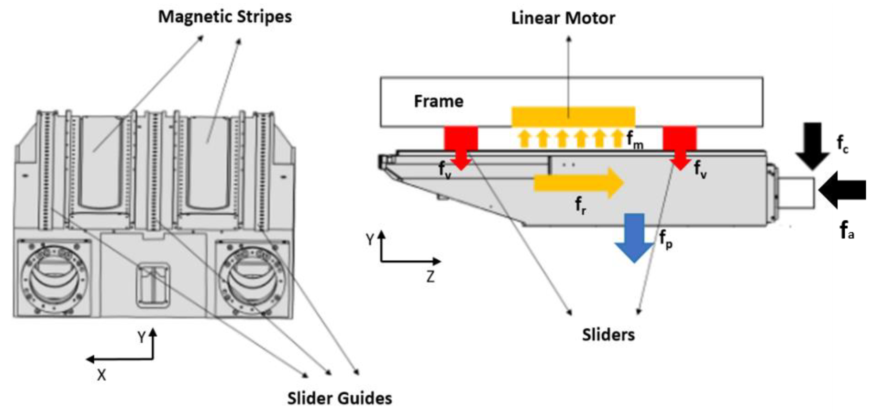
Figure 1 depicts the Z-axis carriage of a multi-spindle CNC machine with two housings for spindles. The carriage is supported by two sliders. In this work, the carriage was considered supported by moving constraint instead of modeling a moving carriage with fixed supports. This assumption does not affect the dynamic behavior of the model and simplifies the development of the model itself.

Two linear motors are integral with the frame and allow the motion along the Z-axis of the machining center. The magnetic stripes of the linear motor are installed on the carriage and the actuation of motion is due to the interaction between the coils of the slider of the linear motor and the magnetic stripes on the carriage.

The sliders are linear motion bearings that constrain the carriage along the transverse directions X and Y, while providing free motion along the Z-axis direction. The magnetic field of the stripes exerts a magnetic force f_r along the Z-axis that accelerates the carriage. As a side effect, a secondary vertical force f_m is also exerted along the Y-axis by the magnetic field. The magnetic force f_m is balanced by the sliders that provide a reaction force f_v in the opposite direction, and by the weight of the carriage f_p. The reaction force f_v and the related displacement in the slider depend on the stiffness of the slider k_s. A force with an axial and a transversal component f_c and f_a is applied at the spindle.

3. Model Description

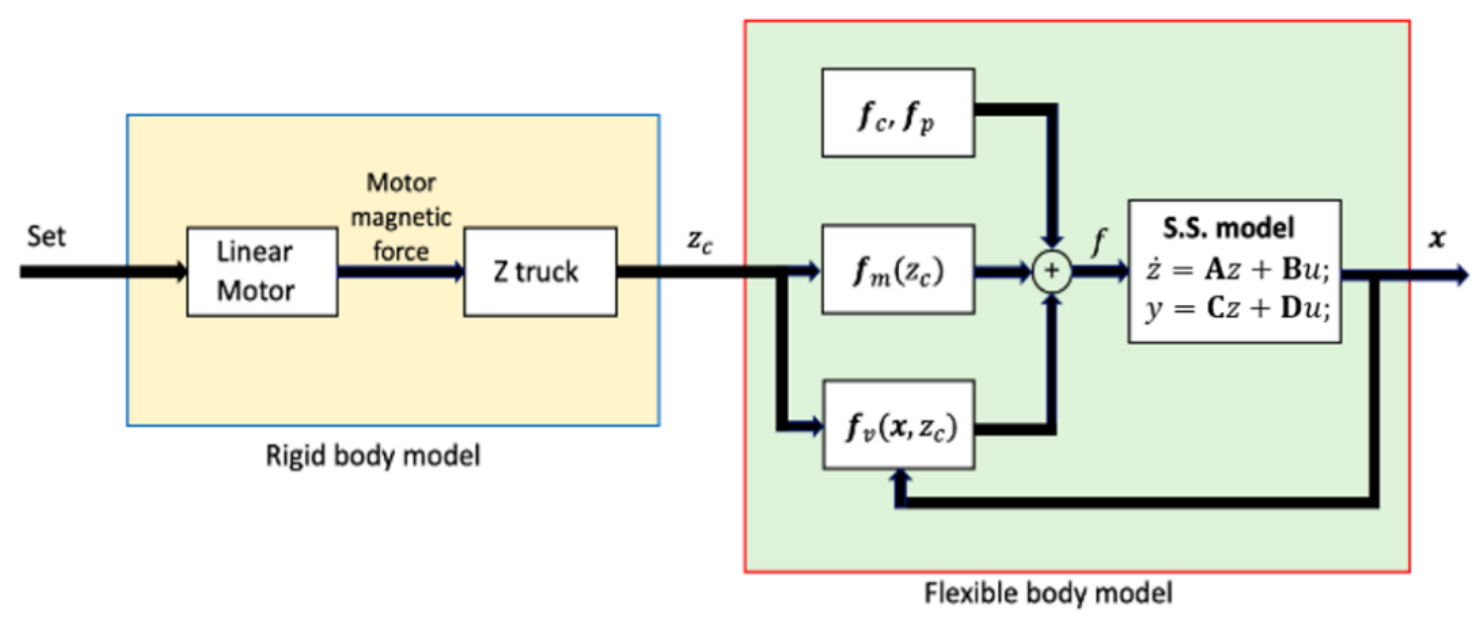
The motion of the carriage is given by the superposition of a rigid body motion (actuated by the linear motors) and vibrations due to its flexibility. These two motions are studied separately and then coupled. Figure 2 shows the block diagrams of the rigid and flexible models. The actuation of the carriage is modeled in Matlab (R2019a, MathWorks, Natick, MA, USA, 2019) considering the electric linear motor. The flexible motion is modeled in the state-space (S.S.) representation. The system is fed with the forces f while the outputs are the position x and velocity $\dot{x}$ of the tool.

The force vector f is composed by four types of forces acting on the carriage:

• the weight force f_p constant in time;
• the magnetic force with components f_m and f_r, due to the linear motor and depending on the position of the carriage according to the action of the control;
• the cutting force f_c between the spindle of the carriage and the workpiece, variable in time according to the machining process, with a possible axial component f_a;
• the slider-guide force f_v, depending both on the Z-axis position of the carriage and on the position x of the nodes currently in contact with the slider.

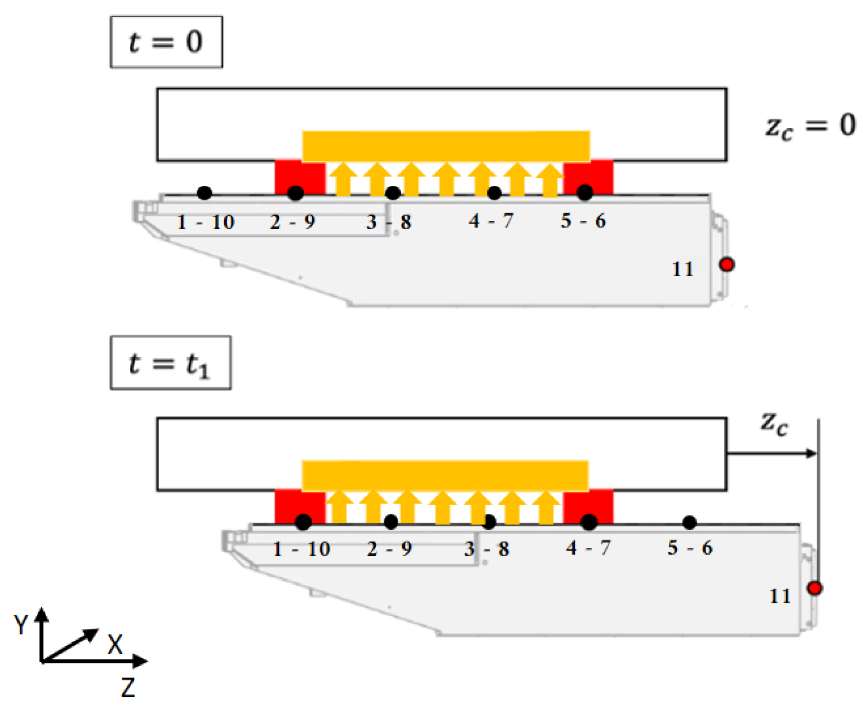
Figure 3 shows the Z-carriage in two different configurations. The numbered nodes were selected as master nodes for the Craig-Bampton reduction of the full FE model of the carriage. This model was developed with a commercial FE software. The Craig-Bampton reduction was performed using the first 20 modes and 11 master nodes. This kind of reduction gives an accurate dynamic behavior of the carriage in the frequency range chosen for the reduction. Since the first modes are the most influencing in dynamic systems, considering 20 modes provides a good approximation. At the same time, mass and stiffness matrices (denoted as M and K, respectively) are small enough to allow fast simulations with an in-house code. Further details on the reduction are reported in [22].

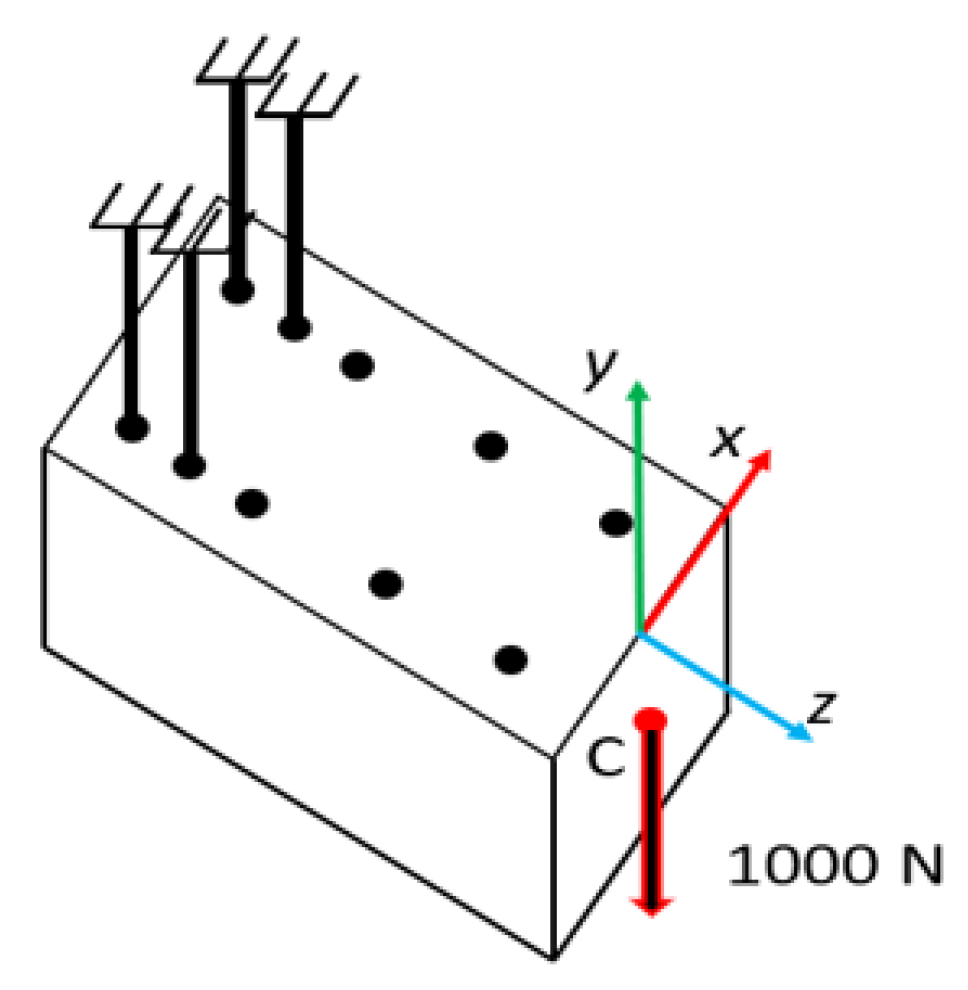
The reduced model of the carriage was compared with the full FE model in the situation as depicted in Figure 3.

As shown in Figure 4, four nodes were constrained along X-, Y- and Z-directions. In Matlab environment, this is expressed adding stiffness in stiffness matrix. The values of the stiffness were assumed 1.58 × 10²⁰ N/m along X- and Z-directions and 1.50 × 10²⁰. N/m along Y-direction. A force equal to 1000 N along the negative direction of the Y-axis is applied on a target node, whose displacement is the element of comparison between the two approaches.

Table 1. Results of the comparison.

	Full FE Model m	Reduced FE Model m
X displacement	1.2726 × 10−15	1.2592 × 10−15
Y displacement	1.3647 × 10−4	1.3647 × 10−4
Z displacement	1.8039 × 10−5	1.8039 × 10−5

shows the results of the comparison in terms of displacements.

When the carriage moves from an initial configuration at time t = 0, in which the Z-coordinate is z_c = 0, to the next configuration at t = t₁ with z_c = z_c1, the relative position of the corresponding nodes on the carriage with the frame changes. Therefore, the magnetic force (in yellow in both Figure 1 and Figure 4) and the constraint due to the sliders (in red in both Figure 1 and Figure 4) are applied to a different set of nodes on the carriage.

3.1. Flexible Model of the System

The reduced model is

$$\left[\begin{array}{cc}{M}_{xx}& M_{x\eta }\\ M_{\eta x}& M_{\eta \eta }\end{array}\right]\left\{\begin{array}{c}{\ddot{x}}_1\\ ⋮\\ {\ddot{x}}_{3N}\\ {\ddot{\eta }}_{3N+1}\\ ⋮\\ {\ddot{\eta }}_{3N+M}\end{array}\right\}+\left[\begin{array}{cc}{K}_{xx}& 0\\ 0& K_{\eta \eta }\end{array}\right]\left\{\begin{array}{c}{x}_1\\ ⋮\\ x_{3N}\\ {\eta }_{3N+1}\\ ⋮\\ {\eta }_{3N+M}\end{array}\right\}=\left\{\begin{array}{c}{f}_1\\ ⋮\\ f_{3N}\\ 0\\ ⋮\\ 0\end{array}\right\}$$

(1)

where K and M are the reduced stiffness and mass matrices, respectively. Throughout this paper, vectors and matrices are denoted by boldface letters. If not explicitly stated otherwise, vectors are column vectors. In the displacement vector indexed elements, x_i represents the displacement along directions X, Y and Z. For the index i, the following rule applies: I = 3(n − 1) + 1, I = 3(n − 1) + 2 and I = 3(n − 1) + 3 corresponds to displacement along X, Y and Z, respectively, where n is the actual master node and N the total number of master nodes. Indexed elements η_j are the modal coordinates, with j = 3N + 1 → 3N + M with M total number of selected modes in the reduction.

The force vector f contains the forces f_i on the master nodes along the three directions, X, Y and Z. The nodal forces on the modal coordinates are zero.

3.1.1. State-Space Representation

It is convenient to use the state-space representation, so that the input of the system is the external forces and constraints, while the outputs are the displacements and velocities of the nodes. The state vector z, the input vector u and the output vector y are:

$$z ={\displaystyle \mathbf{\{}}\mathrm{x};·;\mathrm{x}{\displaystyle \mathbf{\}}};\hspace{1em}u = f;\hspace{1em}y = {\displaystyle \mathbf{\{}}\mathrm{x};·;\mathrm{x}{\displaystyle \mathbf{\}}},$$

(2)

while the state-space representation has the form:

$$\{\begin{array}{c}\dot{z}=\mathbf{A}z+\mathbf{B}u\\ y=\mathbf{C}z+\mathbf{D}u\end{array} ;$$

(3)

the values of the matrices A, B, C and D are obtained by rearranging Equation (1):

$$\left[A\right]= \left[\begin{array}{cc}\mathbf{0}& I\\ -M^{-1}K& \mathbf{0}\end{array}\right]; \left[B\right]=\left[\begin{array}{c}\mathbf{0}\\ -M^{-1}\end{array}\right]; \left[C\right]=\left[\begin{array}{cc}I& \mathbf{0}\\ \mathbf{0}& I\end{array}\right]; \left[D\right]= \left[\begin{array}{c}\mathbf{0}\\ \mathbf{0}\end{array}\right].$$

(4)

3.1.2. External Forces

The forces acting on the carriage are:

• the weight of the carriage f_p;
• the cutting force with components f_c and f_a;
• the magnetic force f_m generated by the linear motor.

In the proposed method, the constraints imposed by the sliders of the carriage have been considered as moving reactions, called slider-guide forces f_v. It will be shown in Section 5 that replacing the physical constraints with the slider-guide forces does not alter the dynamic behavior of the carriage. The carriage was considered to have uniformly distributed mass, so its weight W was equally distributed among the N master nodes. The force is exerted on the vertical axis, downwards, which means that the relative force vector f_p must be filled only in the rows relative to the Y-axis, with negative sign:

$$\left\{f_p\right\}= \left\{W_1\dots W_{3N} 0\right\}$$

(5)

with $W_{3\left(n-1\right)+1}=W_{3\left(n-1\right)+3}=0; W_{3\left(n-1\right)+2}=-\frac{W}{N}; n=1\to N$

The cutting force depends on the machining operation. In a generalized form, it is represented as a sinusoidal function. It is applied only on the node representing the position of the spindle, in vertical direction, when the carriage approaches the position of the workpiece. Its transversal component is f_c = F_c sin(ωt), with ω the spindle speed, in rad/s, and F_c the amplitude of the cutting force. Their value is reported in Section 6.

The magnetic force is exerted in the area, denoted to as magnetic area, located between the middle points of the sliders. The magnetic force on the nodes was modeled with a trapezoidal shape as a function of the position z_c of the carriage. The total magnetic force is given by the sum of all the magnetic forces on the nodes. With a proper choice of the trapezoidal shape, the total magnetic force remains constant when the nodes enter or leave the magnetic area. Nodes outside the magnetic area undergo a null magnetic force. Figure 5 plots the magnetic force perceived by 4 adjacent nodes as a function of the normalized carriage position z_c/z_c,max. For a simplicity’s sake, only two nodes at most were considered to lie in the magnetic area. Considering the magnetic force acting on node 2, the trapezoidal function works as follows (see Figure 5):

• in the area between 0 and A, both node 1 and node 2 are in the magnetic area. Node 2 is entering in the area in position 0 and node 1 is leaving the area in position A. The value of the magnetic force of node 1 is decreasing from the maximum value of the total magnetic force to zero. The value of the magnetic force on node 2, instead, is increasing from zero to the maximum force. The sum of the two force contributions is constant and equal to the value of the total magnetic force; this is evident in position D where both the forces are equal to half of the total magnetic force.
• In the area between A and B, only node 2 is in the magnetic area. The trapezoidal function is constant and equals the total magnetic force.
• In the area between B and C, node 3 enters the magnetic area: the magnetic force on node 3 is increasing and the magnetic force in node 2 is decreasing.

Generalizing, the magnetic force for a master node is developed as follows:

• before entering the magnetic area, a node i does not sense the influence of the magnetic force, so the value of the magnetic function on node i is equal to zero.
• When node i enters the magnetic area, a node (i − 1) is present in the magnetic area; the value of the force on the node i increases from zero in a straight line, and the value of the force on node (i − 1) decreases, following a straight line having the same slope as the previous one, but with opposite sign. This ensures that the sum of the force on nodes is constant and equals the value of the total magnetic force.
• Once the node (i − 1) has left the magnetic area, only node i senses the magnetic force, so the value of the magnetic function is equal to the total magnetic force.
• When node (i + 1) is entering the magnetic area, the value of the magnetic force on node i decreases as already seen for node (i − 1) till it gets equal to zero where it leaves the magnetic area.
• Once node i has left the magnetic area, the value of the function of the magnetic force on node i is equal to zero.

The magnetic force is equal to the sum of the contributions of all the nodes. Developing the functions of the magnetic force on the nodes in the way described ensures that the magnetic force is constant and equal to the total magnetic force, for every position z of the carriage.

When only one node lies in the area between the sliders, the value of the force is equal to the value of the magnetic force. This condition is true in the area where the function is constant in Figure 5.

The magnetic force is considered only along the Y-axis, in positive direction. Therefore, the resulting magnetic force vector is:

$$\left\{f_m\left(z\right)\right\}= \left\{F_{m,1}\left(z\right)\dots F_{m,3N}\left(z\right) 0\right\}$$

(6)

where $F_{m,}{}_{3i+1}=F_{m,}{}_{3i+3}=0; F_{m,}{}_{3i+2}=M;i=0\to \left(N-1\right)$

4. Moving Constraints: Sliding–Guide Force

A multi-degree of freedom (mdof) system can be expressed as:

$$\left[M\right]\left\{\ddot{\mathit{x}}\right\}+\left[K\right]\left\{\mathit{x}\right\}=\left\{\mathit{F}\right\}.$$

(7)

In this particular case, the system in (7) is relative to a free system, in which elastic constraints are not considered. Stiffness matrix K is symmetric and has dimension h × h, with h equal to the number of degrees of freedom (dof). Constraining the mdof system can be obtained adding to K a constraint matrix K_C:

$$\left[K_c\right]=\mathit{d}\mathit{i}\mathit{a}\mathit{g}\left({\mathit{c}}_{\mathbf{1}}, {\mathit{c}}_{\mathbf{2}}, \dots , {\mathit{c}}_{\mathit{a}}\right)$$

(8)

K_C has dimension h × h and it is a diagonal matrix. On its main diagonal, the values of the constraints relative to the different dof are present. System (7) becomes:

$$\left[M\right]\left\{\ddot{\mathit{x}}\right\}+\left(\left[K\right]+\left[K_C\right]\right)\left\{\mathit{x}\right\}=\left\{\mathit{F}\right\},$$

(9)

which rearranging is:

$$\left[M\right]\left\{\ddot{\mathit{x}}\right\}+\left[K\right]\left\{\mathit{x}\right\}=\left\{\mathit{F}\right\}-\left[K_C\right]\left\{\mathit{x}\right\}.$$

(10)

This is the solution chosen to represent a constraint as an external force, considering the stiffness matrix of the free system.

The constraints due to the sliders were introduced in the model using elastic constraints representing the contact stiffness of the slider along the X and the Y axes. The reaction force is given by the contact stiffness times the displacement x of the constrained node. The reaction force is a function of the displacement x, and its point of application depends on the relative position along the Z-axis between the carriage and the frame. The supports are modeled with discretized contact points. Therefore to correctly model the effect of the supports, it is necessary to ensure:

• the continuity of the reaction force during its transition between two neighboring nodes;
• that the total stiffness of the constrained nodes is equal to the total stiffness of the slider.

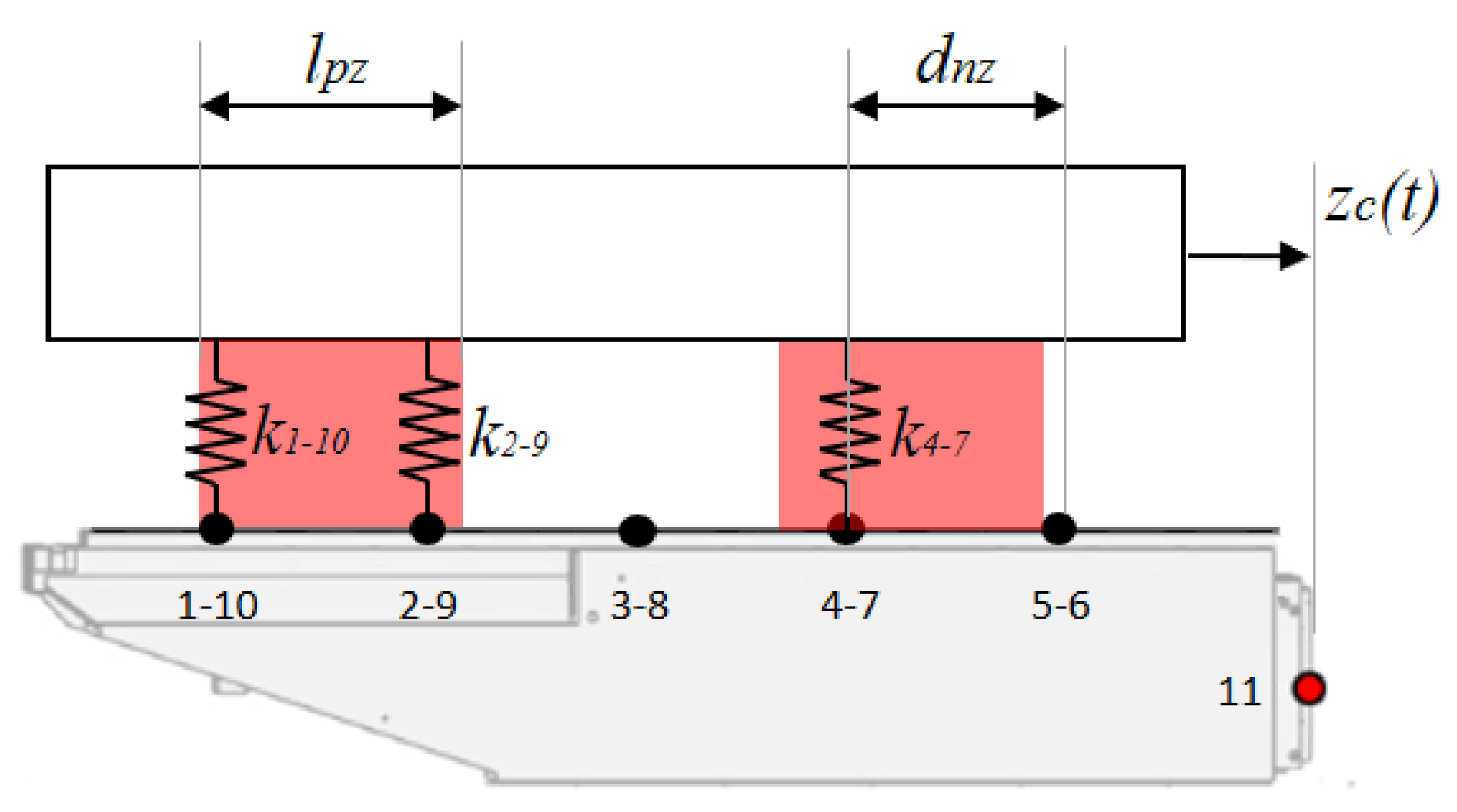
In Figure 6, the slider is represented by stiffness connected to the nodes denoted to as constraining nodes. The constraining nodes depend on the Z-position of the carriage; therefore, the sliders were considered as moving in the reference frame of the carriage. The stiffness was defined as function of the Z-position of the carriage.

To ensure the continuity of the total stiffness of the constraints, the distance between two adjacent nodes must be less than the length of the slider. This condition must be addressed during the reduction step. The nodes must be placed at a distance d_zn included between half the length of the slider l_pz/2 and its total length l_pz, see Figure 6. The slider-guide force along the Y axis can be expressed as:

$$f_v=-k_s\delta ,$$

(11)

with δ the elastic approach of the contact points between the carriage and the slider and k_s the total stiffness of the slider. When there are two nodes in the slider area, the force can be expressed as:

$$f_v=f_{v_1}+f_{v_2}=-k_1{\delta }_1-k_2{\delta }_2=\left(k_1+k_2\right)\delta .$$

(12)

The approaches of the contact points were assumed the same.

The stiffness is represented by the following vector:

• in the rows relative to the modes, the value of the stiffness is equal to zero;
• in the rows relative to the Z-coordinate of the nodes is equal to zero, too, because the carriage is free to move in this direction;
• the x and y rows of each node, instead, are filled with the function expressing the value of the stiffness.

The vector has the form:

$$\left\{K_s\left(\mathrm{z}\right)\right\}=\left\{-{\mathit{K}}_1\left(z\right)\dots -{\mathit{K}}_N\left(z\right) 0\right\}.$$

(13)

with K_i = {k_x,i k_y,i 0}.

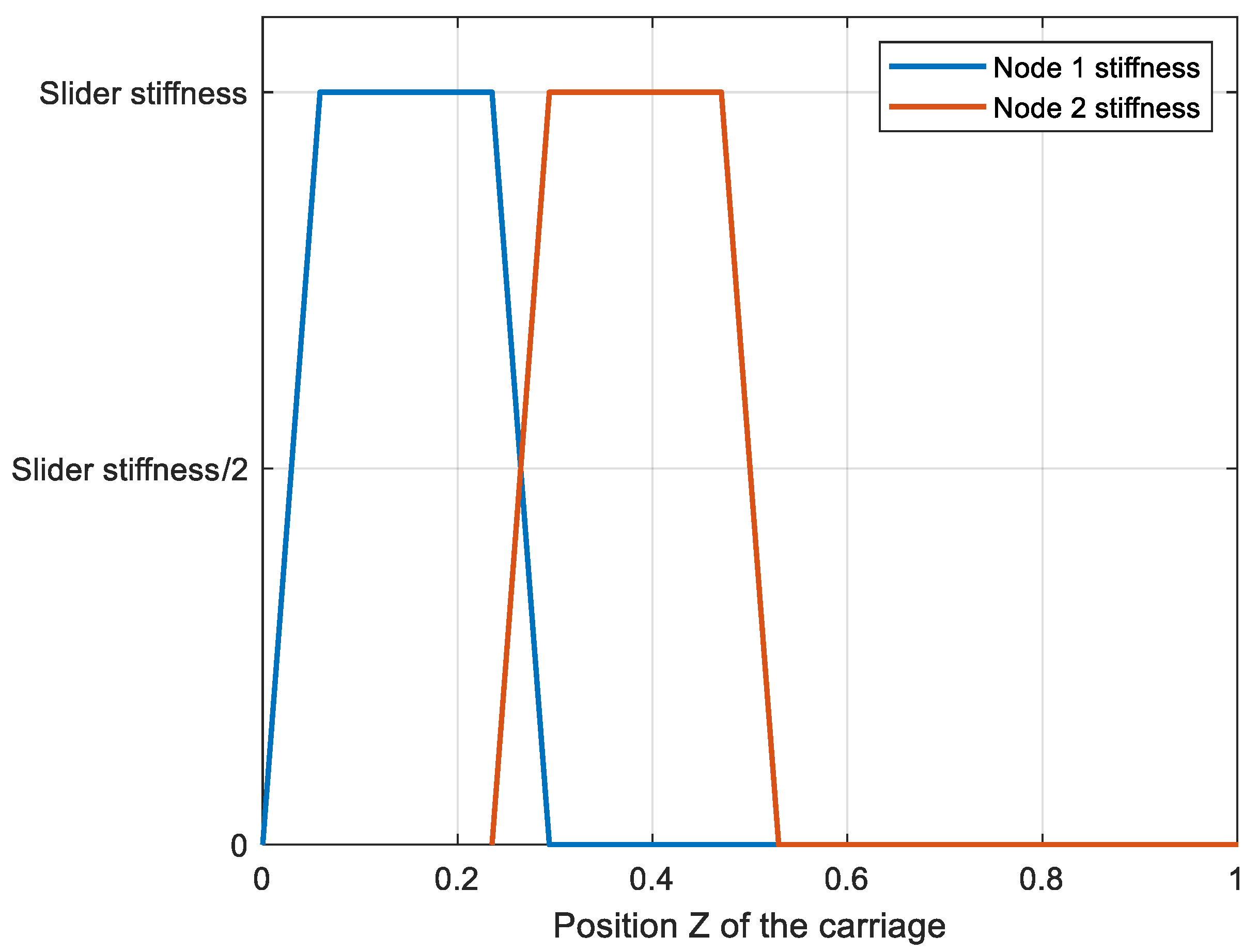
The reaction force due to the elastic constraints can be modeled in a similar way as done for the magnetic force. For this aim, a trapezoidal function was chosen to represent the contact stiffness on a single node. As for the magnetic force, this function equals the total stiffness when only a node is in contact with the slider. The function is zero if the node is outside the contact area. The transition between the two extreme stages is linear and allows to simulate when adjacent nodes enter or leave the contact area. This trapezoidal function was designed so that the total stiffness of the slider is constant.

Considering that only one slider sustains the carriage, the functions of two adjacent nodes are those presented in Figure 7.

When the carriage runs from 0.25 to 0.3, the two nodes are both in full contact with the slider. The stiffness of node 1 decreases to zero while the stiffness of node 2 increases up to the total stiffness of the slider. The two curves have the same slope, with opposite sign. During the transition from full contact at node 1 to full contact at node 2 (the linear part of the trapezoidal function), the sum of the stiffnesses equals the total stiffness of the slider. When only one node is in the contact area (from 0.05 to 0.25, for example) the stiffness of this node equals the total stiffness of the slider.

The stiffness vector has the form:

$$\left\{K_s\left(\mathrm{z}\right)\right\}=\left\{-{\mathit{K}}_1\left(z\right)\dots -{\mathit{K}}_N\left(z\right) 0\right\}.$$

(14)

with K_i = {k_x,i k_y,i 0}.

5. Model of the Body with Moving Constraint

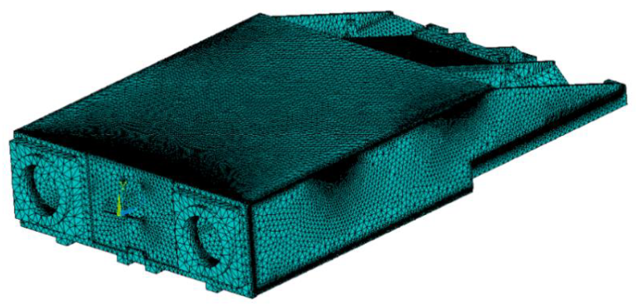
The body meshing of the carriage of the Z-axis is shown in Figure 8.

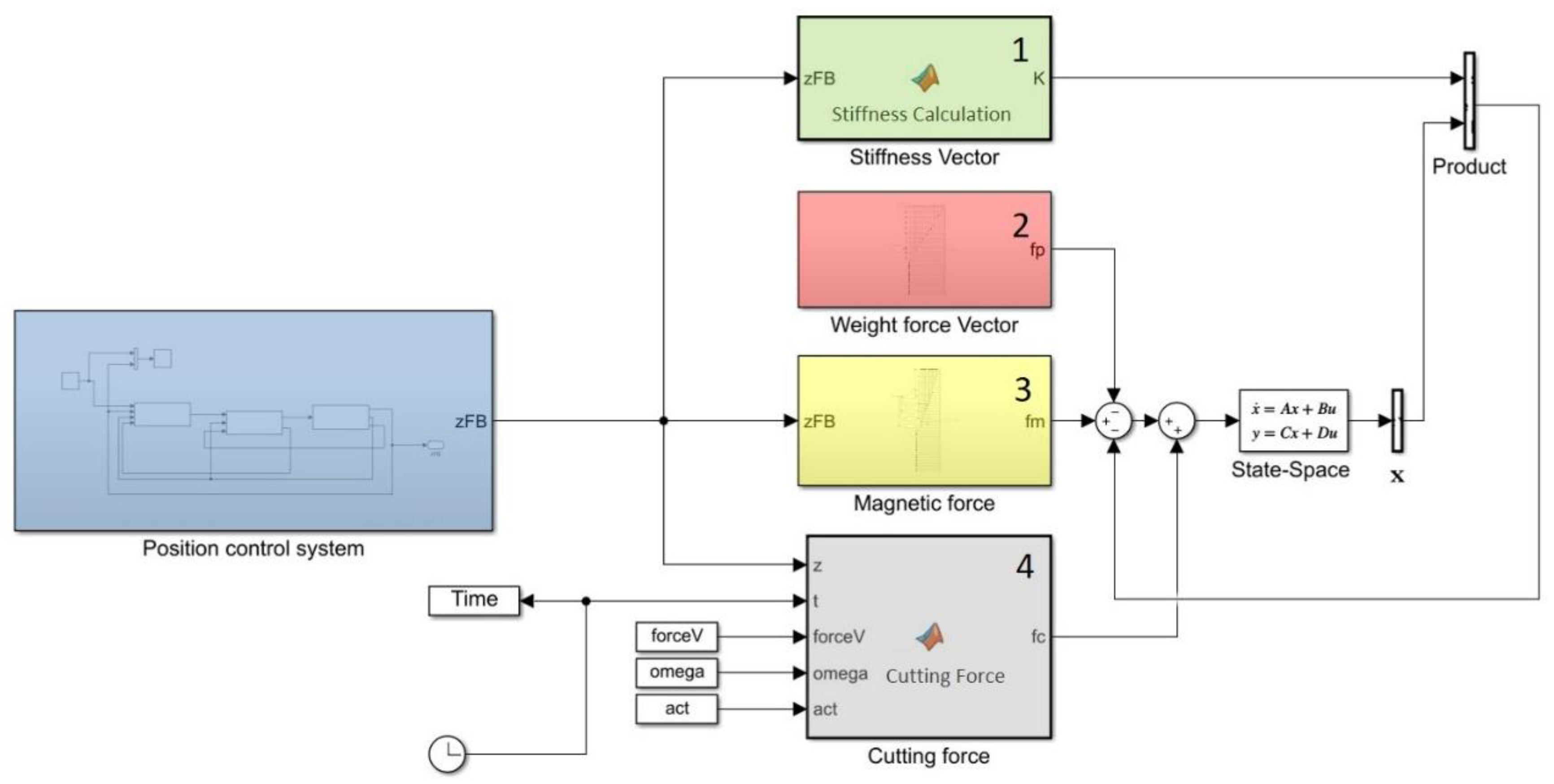
The model described in Section 3 is implemented in Simulink.

The Simulink system used is the one presented in Figure 9. The leftmost subsystem is the position control loop, within which a PID controller provides command to the linear electric drive, while:

• in box 1 the functions relative to the value of the stiffness are calculated;
• in box 2 the weight force vector is assembled;
• in box 3 the magnetic force is computed;
• in box 4 the cutting force vector is evaluated, as a zero vector but on the y-direction of the 11th node (spindle nose node), where the force calculated as:

$$F= \{\begin{array}{c}0 for z<c\\ F_c\sin \left(\omega t\right) for z\ge c\end{array},$$

(15)

with F_c the value of the amplitude of the force, ω the pulsation of the sinusoidal force, z the position of the carriage along Z-direction, and c the target position, where the piece is considered to start being machined.

From the position control system block, the position of the carriage along the Z-direction were derived. This information was the input of the stiffness vector block, of the magnetic force block and of the cutting force block, because, as seen before, the values of the corresponding variables are functions of the Z-position of the carriage. The cutting force inputs were, in addition, the time of the simulation, the amplitude of the force, the spindle speed and the position of the workpiece (in Figure 9, the constant act). The sum of the forces was input for the state-space block. The displacement vector x was the output of the state-space block and it was multiplied by the stiffness vector for sliding-guide force evaluation.

The mean time to complete one second of simulation is around 600 s. Though quite a long time, this made possible to perform many simulations, in order to define a map of the possible errors that can derive when machining a part because of the vibrations of the system. As the carriage moves, the stiffness (and so the complete dynamics) of the system changes as well.

The values used are summarized in

Table 2. Values of the variables of interest of the model.

Variable	Value
Slider Stiffness	2 × 106 N/m
Total Weight Force	132.30 N
Total Magnetic Force	300.00 N
Cutting Force Amplitude	100.00 N

.

The map we are going to present contains the value of the maximum possible error with respect to the position where the cutting process starts and to the frequency ω of the cutting force.

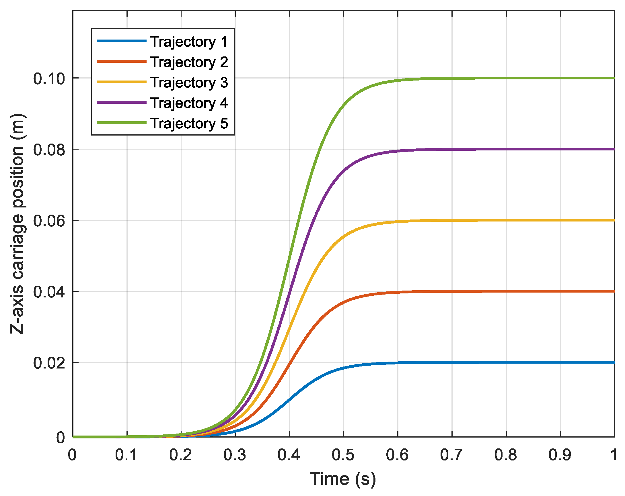
In Figure 10, the five trajectories of the carriage chosen for the realization of the map are shown. These are sigmoid functions, and we assume that the part to cut is in five different positions: 0.02 m, 0.04 m, 0.06 m, 0.08 m and 0.10 m.

Spindles can be divided in:

• spindles with external motor (transmission generally with belts), which run at 12,000 ÷ 15,000 rpm;
• spindles with internal motor (electrospindles), running at 20,000 ÷ 60,000 rpm.

In the following, results relative to both the situations are presented.

6. Results and Discussion

Each simulation considers a step motion of the carriage and the application of a rotating cutting force. The following maps show results for different width of the step motion and for different angular velocity of the spindle.

Data obtained in time simulation are filtered using a band pass filter, to maintain only the information relative to the cutting force.

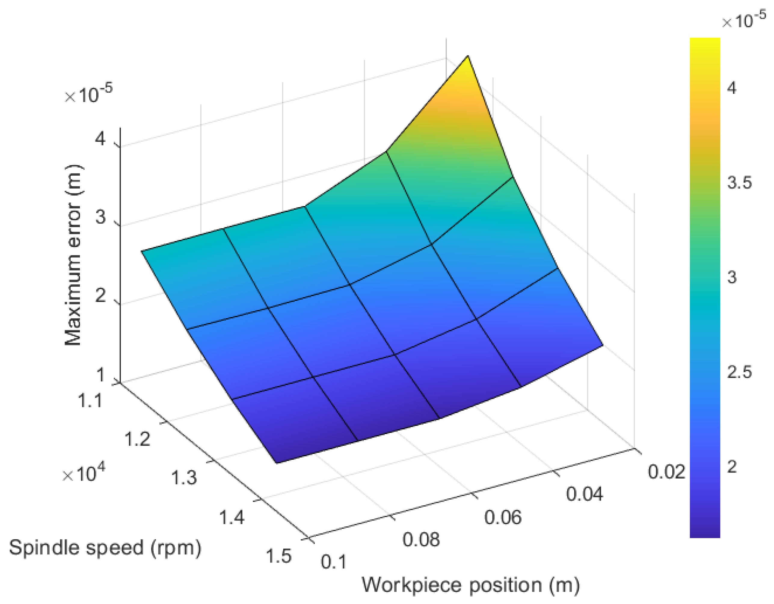
Figure 11 shows the map obtained for an example of spindle with external motor.

The data are collected for a spindle running at a velocity equal to 1200 rad/s, 1300 rad/s, 1400 rad/s and 1500 rad/s. For all the velocities, the higher is the value of the position of the workpiece the lower is the error.

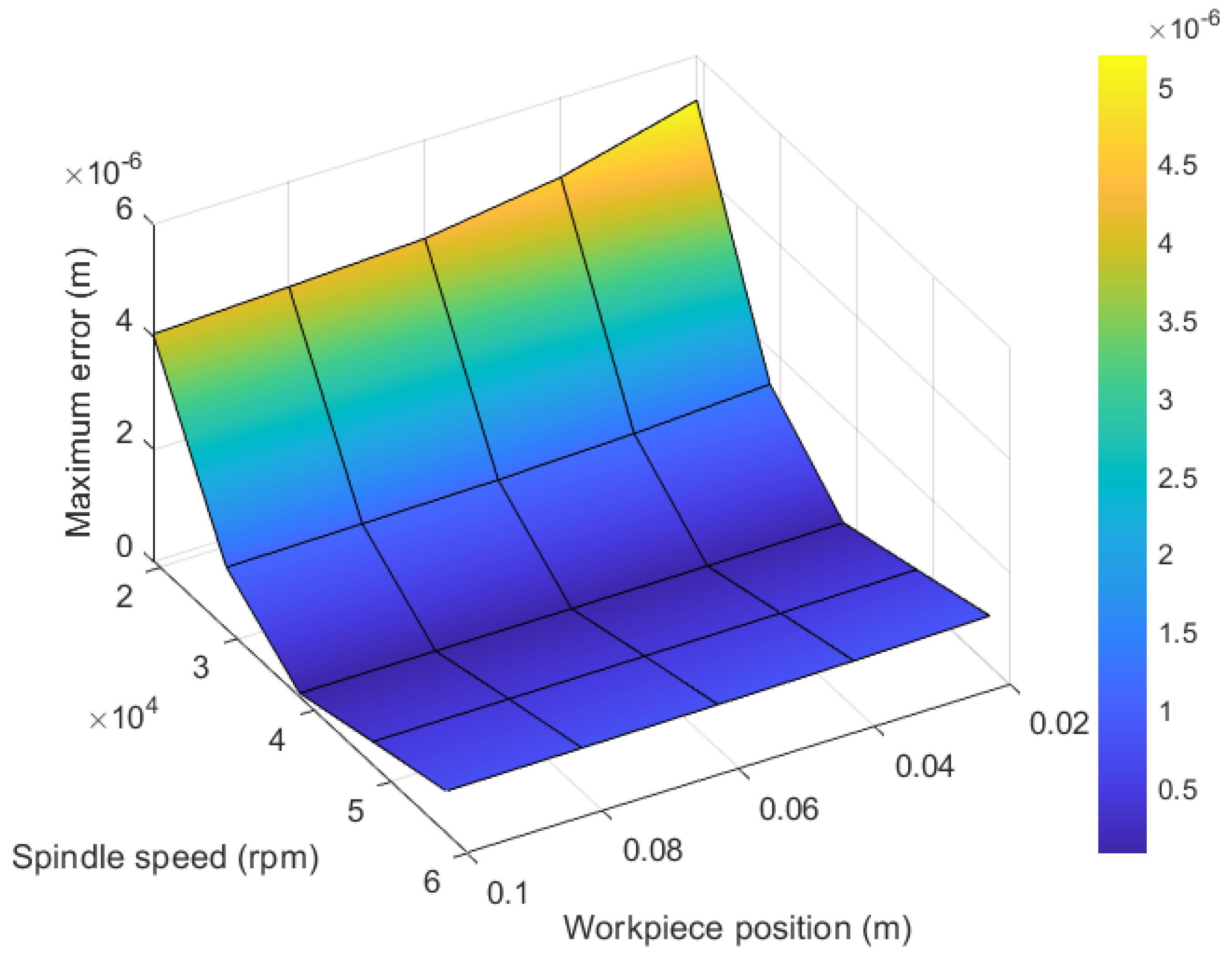
Figure 12, instead, shows the map relative to an example with an electrospindle.

The collected data refer to an electrospindle running at 2000 rad/s, 3000 rad/s, 4000 rad/s and 5000 rad/s. The same reasoning about the position of the carriage holds.

These maps are a very quick instrument to investigate which run that the carriage performs is the best, in order to obtain the minimum error possible. Once the system is built, it is also possible to make tests with different positions of the carriers, changing the values of the forces or changing the design of the carriage, simply substituting the mass and stiffness matrices obtained by FE analysis.

7. Conclusions

The main result of this paper is to suggest a method to model a flexible system in the Matlab/Simulink environment, in order to study its motion control, without requiring the development of a multibody model. This result can be useful as Simulink is a standard simulation environment for control design. The proposed method can be applied in those cases in which vibrations can have a significant impact on the performance of a controlled system, making rigid body simulation unsatisfactory for the purpose of control design.

The suggested method considers the use of a reduced dynamic model of the flexible body obtained by reducing a full FE model with the Craig-Bampton method.

As a case study, the carriage of a machining center was considered. The carriage is powered by a linear electric motor and it is supported by a pair of sliders that provide moving constraints and modify the dynamic behavior of the assembly. The problem of the moving constraints has been treated in an original way. The constraints were introduced in the system as external forces given by the stiffness of the supports. A trapezoidal function was introduced to simulate the stiffness of the supports. This function was designed so that the total stiffness is constant as the carriage moves along its Z-axis. A similar solution was introduced to model the magnetic force exerted by the linear motor on the carriage along the transverse Y-direction.

The Craig-Bampton reduced dynamic model consists of 53 degrees of freedom instead of the thousands dofs of the full model, and the outputs were proven to be close to those provided by the complete model.

The complete model can run a 1 s simulation in 600 s, making possible its use for control design and parametric analysis of the system.

References

- Shabana, A.A. Flexible multibody dynamics: Review of past and recent developments. Multibody Syst. Dyn. 1997, 1, 189–222. [Google Scholar] [CrossRef]
- Wallrapp, O. Flexible bodies in multibody system codes. Veh. Syst. Dyn. 1998, 30, 237–256. [Google Scholar] [CrossRef]
- Hu, F.L.; Ulsoy, A.G. Dynamic modeling of constrained flexible robot arms for controller design. J. Dyn. Syst. Meas. Control. Trans. ASME 1994, 116, 56–65. [Google Scholar] [CrossRef]
- Omar, M.A. Modeling flexible bodies in multibody systems in joint-coordinates formulation using spatial algebra. Adv. Mech. Eng. 2014, 2014. [Google Scholar] [CrossRef]
- Ferretti, G.; Schiavo, F.; Viganò, L. Modular modelling of flexible thin beams in multibody systems. In Proceedings of the 44th IEEE Conference on Decision and Control, and the European Control Conference, CDC-ECC ‘05, Seville, Spain, 12–15 December 2005. [Google Scholar] [CrossRef]
- Mukherjee, R.M.; Anderson, K.S. A logarithmic complexity divide-and-conquer algorithm for multi-flexible articulated body dynamics. J. Comput. Nonlinear Dyn. 2007, 2, 10–21. [Google Scholar] [CrossRef][Green Version]
- Hosseinabadi, A.H.H.; Altintas, Y. Modeling and active damping of structural vibrations in machine tools. CIRP J. Manuf. Sci. Technol. 2014, 7, 246–257. [Google Scholar] [CrossRef]
- Wang, X.; Mills, J.K. A FEM model for active vibration control of flexible linkages. In Proceedings of the IEEE International Conference on Robotics and Automation 2004 (ICRA ‘04), New Orleans, LA, USA, 26 April–1 May 2004. [Google Scholar] [CrossRef]
- Arisoy, A.; Gökasan, M.; Bogosyan, O.S. Tip position control of a flexible-link arm. Int. Work. Adv. Motion Control. AMC 2006, 445–450. [Google Scholar] [CrossRef]
- Jnifene, A. Active vibration control of flexible structures using delayed position feedback. Syst. Control Lett. 2007, 56, 215–222. [Google Scholar] [CrossRef]
- Fernando, J.; Solís, P.; Navarro, G.S.; Linares, R.C. Modeling and tip position control of a flexible link robot: Experimental results. Comput. Sist. 2009, 12, 421–435. [Google Scholar] [CrossRef]
- Neugebauer, R.; Scheffler, C.; Wabner, M.; Schulten, M. Advanced state space modeling of non-proportional damped machine tool mechanics. CIRP J. Manuf. Sci. Technol. 2010, 3, 8–13. [Google Scholar] [CrossRef]
- Bianchi, G.; Cagna, S.; Cau, N.; Paolucci, F. Analysis of vibration damping in machine tools. Procedia CIRP 2014, 21, 367–372. [Google Scholar] [CrossRef]
- Neugebauer, R.; Scheffler, C.; Wabner, M. Implementation of control elements in FEM calculations of machine tools. CIRP J. Manuf. Sci. Technol. 2011, 4, 71–79. [Google Scholar] [CrossRef]
- Gao, X.; Zhang, Y.; Zhang, H.; Wu, Q. Effects of machine tool configuration on its dynamics based on orthogonal experiment method. Chin. J. Aeronaut. 2012, 25, 285–291. [Google Scholar] [CrossRef]
- Allotta, B.; Angioli, F.; Rinchi, M. Constraints identification for vibration control of time-varying boundary conditions systems. In Proceedings of the 2001 IEEE/ASME International Conference on Advanced Intelligent Mechatronics, Como, Italy, 8–12 July 2001. [Google Scholar] [CrossRef]
- Brecher, C.; Fey, M.; Tenbrock, C.; Daniels, M. Multipoint constraints for modeling of machine tool dynamics. J. Manuf. Sci. Eng. Trans. ASME 2016, 138, 1–8. [Google Scholar] [CrossRef]
- Miller, S.; Soares, T.; Van Weddingen, Y.; Wendlandt, J. Modeling Flexible Bodies with Simscape Multibody Software An Overview of Two Methods for Capturing the Effects of Small Elastic Deformations. Available online: https://it.mathworks.com/campaigns/offers/model-flexible-bodies.html?elqCampaignId=10588# (accessed on 7 January 2019).
- Botto, D.; Lavella, M. A numerical method to solve the normal and tangential contact problem of elastic bodies. Wear 2015, 330–331, 629–635. [Google Scholar] [CrossRef]
- Botto, D.; Lavella, M. High temperature tribological study of cobalt-based coatings reinforced with different percentages of alumina. Wear 2014, 318, 89–97. [Google Scholar] [CrossRef]
- Mauro, S.; Pastorelli, S.; Mohtar, T. Sensitivity analysis of the transmission chain of a horizontal machining tool axis to design and control parameters. Adv. Mech. Eng. 2014, 6, 1–8. [Google Scholar] [CrossRef]
- Haile, W.B. Craig-Bampton Method an Introduction To Boundary Node Functions, Base Shake Analyses, Load Transformation Matrices, Modal Synthesis and Much More. Available online: https://femci.gsfc.nasa.gov/craig_bampton/Primer_on_the_Craig-Bampton_Method.pdf (accessed on 7 January 2019).
© 2020 by the authors. Licensee MDPI, Basel, Switzerland. This article is an open access article distributed under the terms and conditions of the Creative Commons Attribution (CC BY) license (http://creativecommons.org/licenses/by/4.0/).