Abstract
Degraded electrodes in a resistance spot welding system should be replaced to ensure that weld quality is maintained. Welding electrodes are subjected to different environmental and operational loading conditions during use. When they are replaced with a fixed interval, replacement may occur too early (raising maintenance costs) or too late (leading to quality issues). This motivates condition monitoring strategies for resistance spot welding electrode tips. Thus, this paper proposes a modified recurrence plot (RP) for robust condition monitoring of welding electrode tips in resistance spot welding systems. The overall procedure for the proposed condition monitoring approach consists of three steps: (1) transformation of a one-dimensional signal to a two-dimensional image, (2) unsupervised feature extraction with LeNet architecture-based convolutional neural networks, and (3) health indicator calculation. RP methods convert dynamic resistance waveforms to RPs. The original RP method provides an image with binary-colored pixels (i.e., black or white) that makes this method insensitive to the change of the waveform signal. The proposed RP method is devised to be sensitive to the change of the waveform signal, while enhancing robustness to external noise. The performance of the proposed RP method is evaluated by examining simulated aperiodic waveform signals with and without external noise. A case study is presented to examine the proposed method’s ability to monitor the condition of resistance spot welding electrodes. The results show that the proposed method outperforms handcrafted, feature-based condition monitoring methods. This study can be used to accurately determine the lifetime of welding electrodes in real time during the spot welding process.
1. Introduction
Spot welding is widely used in various industrial fields, such as automobile assembly lines, ship building, and automated manufacturing facilities. The quality of spot welds is critical to the structural integrity and safety of the welded products. Poor-quality welds, which may occur due to improper setting of welding parameters and adversarial environmental conditions, can lead to catastrophic failure of engineered products [1]. Therefore, it is important to secure weld quality during the spot welding process. To this end, an efficient testing method for spot welds is desired.
Spot weld testing methods can be divided into destructive testing and nondestructive testing [2]. Destructive testing can provide a sufficient amount of direct evidence on weld quality. However, it cannot be performed on welds in every product, since samples have to be inspected in a destructive manner. Therefore, destructive testing is only applicable for inspecting a small number of products sampled from a population of products.
Nondestructive testing can be conducted by visual inspection. Visual inspection can be conducted with radiographs of the welding pool [3] and images taken from welding electrode tips [4]. The welding pool radiograph can be used to identify discontinuities that correspond to different types of defects. The wearout of welding electrode tips is evaluated by examining the changes in the relative radius of the welding electrode tip in the images. Image data provide information that is useful for monitoring the welding quality during the spot welding process [5]. However, the results from visual inspection can often be unreliable due to adversarial environmental conditions, such as surface contamination [6]. Thus, nondestructive testing by visual inspection has had limited success in industry.
Another nondestructive testing method is to analyze waveforms taken from mechanical and electric signals during spot welding, e.g., ultrasonic signals [7], dynamic resistance [8], electrode displacement [9], and electrode force [10]. Among them, dynamic resistance waveforms have commonly been employed to evaluate weld quality since they are robust to external noise [11,12]. Dynamic resistance directly represents the physical characteristics of the spot welding process. Dynamic resistance waveforms during the spot welding process are divided into three regions. First, the dynamic resistance drops rapidly when the electric current starts to flow. Second, the dynamic resistance of the welding electrode increases due to the increase in the temperature of the welding spot. Finally, the dynamic resistance of the welds decreases as the molten metal bond grows. It should be noted that waveforms contain valuable information regarding the dynamic change in a system.
Numerous researchers have attempted to find the best feature that presents the condition of welding electrode tips. Several handcrafted features—including half-cycle peak, maximum, slope, mean, and standard deviation—have been proposed in prior work [1,13,14]. However, it is challenging to develop a single feature that represents the whole process. To address this challenge, a combination of various handcrafted features that use principal component analysis [15] and neural networks [16] have been developed. Nonetheless, there is not yet a universal feature (or health indicator) for monitoring welding electrode tips in a spot welding system.
The type of waveforms can be generally divided into stationary and non-stationary as shown in Figure 1. The stationary waveforms can be further categorized into random, periodic, and quasi-periodic. Periodic and quasi-periodic waveforms are deterministic and made up of discrete sinusoidal components. The non-stationary waveforms can be grouped into transient, cyclostationary, and continuously varying. Cyclostationary waveforms are an amplitude modulated white noise. To understand the characteristic of the waveforms, appropriate signal processing techniques should be used. For example, periodic and quasi-periodic waveforms can be visualized in one-dimensional (1D) space (i.e., the frequency domain) using Fourier transform (FT), while nonstationary waveforms can be plotted in two-dimensional (2D) space using wavelet transform (WT) and Wigner-Ville distribution (WVD). If nonstationary waveforms are analyzed using FT, the changes in frequency with time will be ignored as FT integrates the waveform over all time. Therefore, a proper technique should be selected by the user depending on the type of waveforms. However, it is challenging to select the most relevant signal technique since the dynamics of an engineered system are often complex and multiple waveform types exist in data collected from the system.
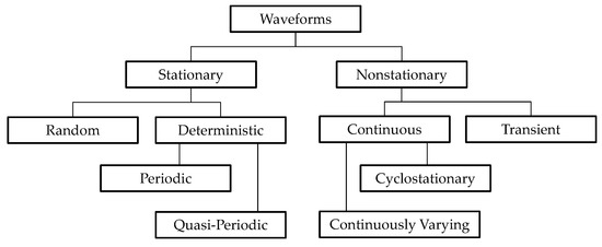
Figure 1.
Waveform types [17].
The state of engineered systems usually changes in time. The study of complex dynamics can help describe, forecasting such changes. A dynamical system can be described by (1) a phase space, (2) a continuous or discrete time and (3) a time-evolution law [18]. Suppose that the state x of a system at a fixed time t can be defined by d components.
where is the vector in the d-dimensional phase space of the system. As an example, for the dynamic resistance waveform reduces to the scalar in a single dimensional phase space.
For time-continuous systems, the time evolution is described by a set of differential equations:
In general, a system returns to former states. A recurrence is a fundamental characteristic of dynamical systems. The method of recurrence plots (RPs) [19] received significant attentions in the fields of engineering [20], biology [21], and neuroscience [22]. RPs that visualize trajectories in the phase space are especially advantageous in the case of high dimensional systems. Other signal processing techniques (e.g., FT, WT, and WVD) mentioned above can visualize only the state of a single dimensional system, not the state of high dimensional systems.
Recently, convolutional neural networks (CNNs), such as VGG-16 [23] and ResNet [24], have shown excellent performance for classifying hundreds and thousands of images. Unlike traditional feature engineering, CNNs can be used to extract features in an unsupervised manner (i.e., unsupervised feature engineering) that does not require human experience. An objective interpretation regarding images of RP structures can be made. Therefore, it is worth examining a combination of RP imaging technique and CNN for monitoring welding electrode tips in a spot welding system.
Motivated by this need, this paper proposes a methodology that can be used to evaluate the condition of welding electrode tips during the spot welding process. First, the waveform is extracted from the dynamic resistance during the spot welding process. To maximize the representation capability of waveforms, one-dimensional (1D) waveforms are converted into two-dimensional (2D) images. The overall procedure consists of (1) waveform imaging; (2) unsupervised feature extraction; and (3) welding electrode condition assessment. The rest of this paper is organized as follows. Section 2 describes the proposed methodology. Section 3 examines the proposed method using a case study of a real spot welding system. Section 4 concludes this paper and discusses future work.
The contributions of this paper can be summarized into two primary areas. First, a new recurrence plot (RP) that converts 1D waveforms into 2D images is proposed to increase the sensitivity of weak signals, while suppressing the effect of external noise. Second, a new methodology is proposed to assess the health condition of welding electrode tips in an unsupervised manner. Waveform signals collected from healthy welding electrode tips in a spot welding system are the only requirement of the proposed method.
2. Proposed Methodology
This section proposes a methodology that combines waveform imaging with deep learning to monitor the health condition of welding electrode tips in a spot welding system. The proposed methodology consists of three steps: (1) waveform imaging, (2) unsupervised feature extraction by CNNs, and (3) welding electrode tip condition assessment. The overall procedure is shown in Figure 2. The condition monitoring signals can be selected with the criteria of (1) ease of data acquisition, (2) correlation with welding electrode condition, and (3) robustness of the data. In the area of nondestructive testing, 1D waveforms (e.g., dynamic resistance, electrode displacement, electrode force, and ultrasonic signals) are commonly employed. First, the 1D waveforms are converted into 2D images. As discussed in the previous section, several waveform imaging methods exist. This study proposes a novel imaging method that is modified from the original RP imaging method. The proposed RP imaging method is devised to improve sensitivity to weak changes in a nonstationary signal and to enhance robustness to external noise. Second, CNNs are used for unsupervised feature engineering. Next, a pre-trained CNN is used to develop activation maps. Finally, a health indicator that assesses the condition of the welding electrode tips is built using the Mahalanobis distance (MD) that is calculated using the outputs from the activation maps.
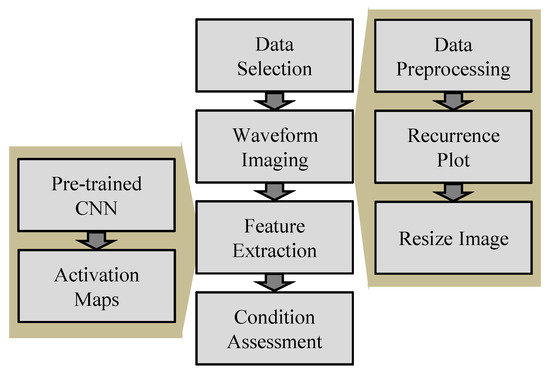
Figure 2.
Flowchart of the proposed methodology.
Section 2.1 describes the process of waveform imaging using the proposed RP method. Section 2.2 outlines the proposed approach for unsupervised feature extraction using pre-trained CNNs. Section 2.3 shows welding electrode tip condition assessment with MD.
2.1. Waveform Imaging Using a Modified Recurrence Plot
Recurrence plot (RP) is a method that can visualize the periodic nature of dynamical systems. To visualize a trajectory of the dynamical system in m-dimensional space (m: integer), the trajectory should be projected on a 2D or 3D sub-space. For example, a trajectory of the dynamical system in a one-dimensional (1D) space can be projected to a 2D or 3D space. RPs are advantageous over other signal processing techniques (e.g., FT, WT, and WVD) since RPs can capture various patterns such as stationary, periodic/quasi-periodic, cyclostationary, and fluctuations. FT fails to capture the characteristic of cyclostationary waveforms. In this study, the trajectory in phase space corresponds to the dynamic resistance waveform acquired from a resistance spot welding system. The RP method enables conversion of waveforms into 2D images.
Let x(i) be the ith data point of the 1D waveform where i = 1, …, K; K is the number of data points. In the same manner, x(j) is the jth data point of the 1D waveform, where j = 1, …, K. The RP matrix at the ith row and the jth column is defined as [18]:
where ε is the predefined threshold (ε > 0). When x(j) is sufficiently close to x(i), one is placed at the ith row and the jth column of the matrix. Otherwise, zero is placed.
The original RP (Ro (i, j)) was introduced to present the closeness of two data points whose output is binary. However, the original RP cannot present the evolution of states between two data points, since the outcome from the original RP is either one or zero. In reality, dynamic resistance waveforms from spot welding systems show gradual changes due to the dynamic nature of the systems, as well as due to external noise. To incorporate the evolution of the system behavior, a modified RP is proposed:
where i and j are the vectors of the waveform data points, respectively; N is the predefined threshold (N > 0); and Rp (i, j)) is the proposed RP matrix at the ith row and the jth column. The proposed RP is devised to give a fixed value of N when the difference between x(i) and x(j) is larger than the threshold N. Otherwise, the difference is the output value of the modified RP.
To compare the performance of the original RP and the proposed RP, simulation studies were conducted with two different types of waveform signals. The signals examined included (1) the positive half cycle of the sinusoidal waveforms and (2) the waveforms that emulate the evolution of dynamic resistance during resistance spot welding. The positive half cycles of the sinusoidal waveforms are shown with different amplitudes f(x), 2f(x), and 4f(x) in Figure 3. As shown in Figure 4, both the original and proposed RP show that the yellow area increases as the amplitude of the simulated waveforms increases. However, the rate of increase in the yellow area for the proposed RP is larger than that for the original RP. Therefore, it was verified that the proposed RP is more sensitive to the amplitude change of waveforms than the original RP.
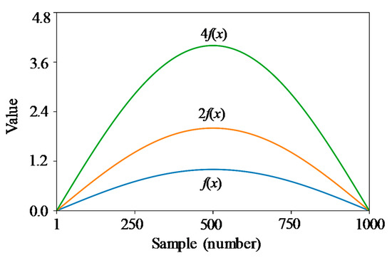
Figure 3.
Simulated aperiodic signals.
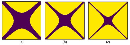
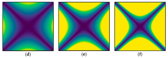
Figure 4.
RP images of simulated aperiodic signals: (a) original RP of f(x), (b) original RP of 2f(x), (c) original RP of 4f(x), (d) proposed RP of f(x), (e) proposed RP of 2f(x), and (f) proposed RP of 4f(x).
To understand the effect of the random noise from external sources on the proposed RP, random noise was added to the simulated waveforms. Three cases are shown in Figure 5: (1) 2f(x), (2) 2f(x) + w(x), and (3) 2f(x) + 2w(x). The yellow area from the original RP fluctuated as the amplitude of the random noise increased, as is shown in Figure 6a–c. However, the yellow area from the proposed RP did not show any significant change as the amplitude of the noise increased; this is depicted in Figure 6d–f. Therefore, it was verified that the proposed RP is more robust to random noise than the original RP. It is worth noting that the yellow area of the proposed RP kept the shape under noisy conditions while the original RP did not.
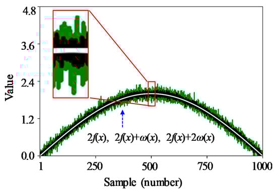
Figure 5.
Simulated aperiodic signals with random noise.
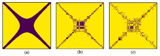
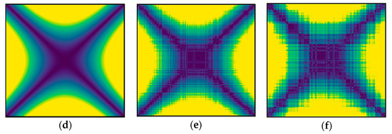
Figure 6.
RP images of simulated noisy aperiodic signals: (a) original RP of 2f(x), (b) original RP of 2f(x) + ω(x), (c) original RP of 2f(x) + 2ω(x), (d) proposed RP of 2f(x), (e) proposed RP of 2f(x) + ω(x), and (f) proposed RP of 2f(x) + 2ω(x).
From visual inspection, it was observed that the yellow area from the proposed RP was more sensitive to amplitude change of the waveforms, while the proposed RP was more robust to random noise. To quantitatively verify the relationship, the yellow area ratio was calculated by dividing the number of pixels of the yellow area by the total number of pixels. As shown in Figure 7 and Table 1, the increase of the yellow area’s ratio between f(x) and 4f(x) using the proposed RP was 56.43% (= 56.65%–0.22%); whereas, the increase using the original RP was only 24.95% (= 87.74%–62.79%). These results show that the proposed RP was twice as sensitive to the amplitude change of the simulated waveform. For the original RP with no random noise, w(x), and 2w(x) random noise, the yellow area increased to 78.39%, 93.95%, and 94.64%, respectively. However, for the proposed RP with no random noise, w(x), and 2w(x) random noise, the yellow area did not show such an increase; results were 29.54%, 29.70%, and 29.86%, respectively. Therefore, it was concluded that the proposed RP is sensitive to amplitude changes of the simulated waveform, while being robust to random noise.
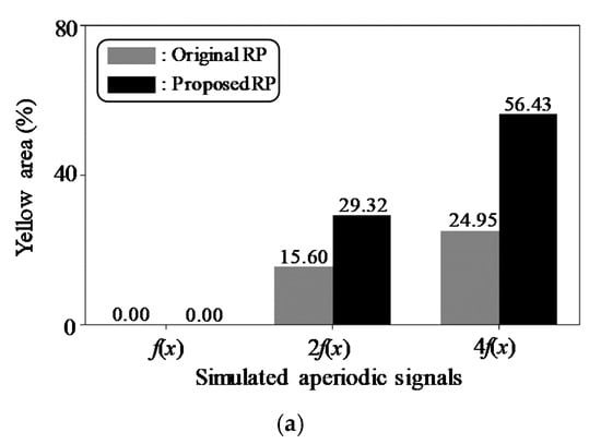
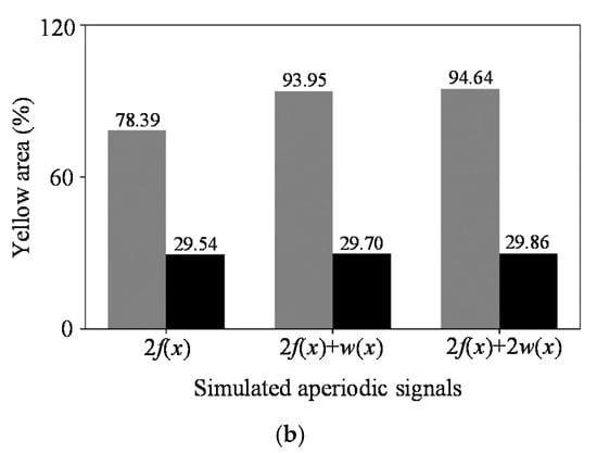
Figure 7.
Performance comparison of the original and proposed RPs using a simulated aperiodic waveform: (a) the change of yellow area as the waveform amplitude increases and (b) the change of yellow area as the random noise increases.

Table 1.
Comparison of yellow area ratio for a simulated aperiodic waveform.
The performance of the proposed RP was also evaluated using another type of waveform signal that emulates the evolution of the dynamic resistance signals during resistance spot welding. We followed a procedure similar to that used for analysis of the simulated aperiodic signals. As presented in Figure 8 and Figure 9, it was visually observed that the proposed RP is more sensitive to the amplitude change of waveforms than the original RP. As depicted in Figure 10 and Figure 11, it was visually verified that the proposed RP is more robust to random noise than the original RP.
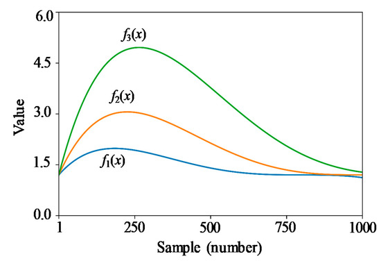
Figure 8.
Simulated dynamic resistance signals.
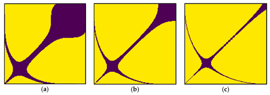
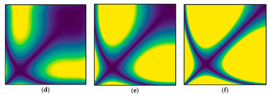
Figure 9.
RP images of simulated dynamic resistance signals: (a) original RP of f1(x), (b) original RP of f2(x), (c) original RP of f3(x), (d) proposed RP of f1(x), (e) proposed RP of f2(x), and (f) proposed RP of f3(x).
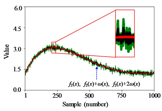
Figure 10.
Simulated dynamic resistance signals with random noise.
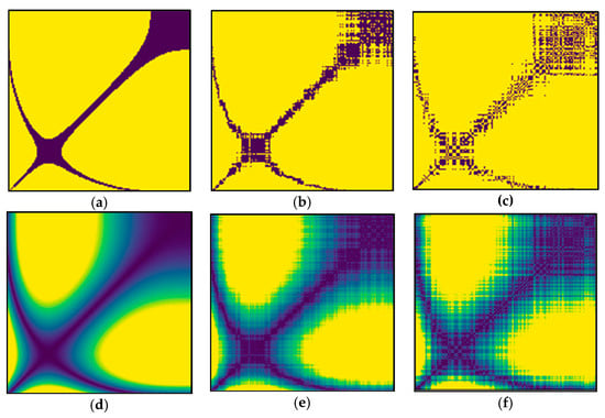
Figure 11.
RP images of simulated noisy dynamic resistance signals: (a) original RP of f2(x), (b) original RP of f2(x) + ω(x), (c) original RP of f2(x) + 2ω(x), (d) proposed RP of f2(x), (e) proposed RP of f2(x) + ω(x), and (f) proposed RP of f2(x) + 2ω(x).
To quantitatively verify the relationship, the yellow area ratio was calculated. As shown in Figure 12 and Table 2, the increase of the yellow area’s ratio between f1(x) and f3(x) using the proposed RP was 21.75% (= 93.68%–71.93%); whereas, the increase using the original RP was only 45.06% (= 59.23%–14.17%). These results show that the proposed RP was three times more sensitive to the amplitude change of the simulated waveform. For the original RP with no random noise, w(x), and 2w(x) random noise, the yellow area increased to 86.97%, 87.73%, and 89.51%, respectively. However, for the proposed RP with no random noise, w(x), and 2w(x) random noise, the yellow area showed a relatively small change; results were 36.41%, 36.50%, and 36.39%, respectively. Therefore, it was concluded that for another type of signal that emulates dynamic resistance waveforms, the proposed RP is sensitive to amplitude changes of the simulated waveform, while being robust to random noise. In summary, an identical conclusion can be drawn from both simulation studies, which examined two different types of waveform signals.
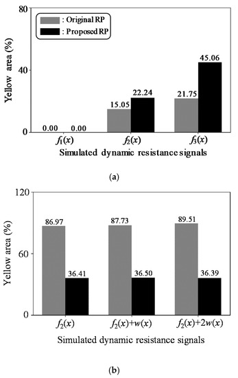
Figure 12.
Performance comparison of the original and proposed RPs using a simulated dynamic resistance waveform: (a) the change of yellow area as the waveform amplitude increases and (b) the change of yellow area as the random noise increases.
Table 2.
Comparison of yellow area ratio for a simulated dynamic resistance waveform.
RPs reveal different patterns (i.e., topology and texture) for phase space trajectories with randomness, periodicity, chaos, and trend as shown in Table 3. For example, single isolated points indicate that strong fluctuation exists in the process. Another example is that diagonal lines parallel to the line of identity (LOI) represent that the evolution of the states is similar at different epochs; the process can be deterministic. RP structures should be quantified with more objective criteria. Marwan et al. [18] states that “the visual interpretation of RPs requires some experience”. It is challenging to interpret the image of RP structures by naked human eyes. Moreover, interpretation results can be changed since personal experiences are different.
Table 3.
Typical pattern in RPs and meanings [18].
2.2. Unsupervised Feature Extraction by CNN
Convolutional neural networks (CNNs) are artificial neural networks that incorporate convolution (in fact, cross correlation) operations. By using the convolution operations, the spatial information of the 2D data can be preserved. The initial layers of convolutional neural networks learn low-level features, such as edges, while the deeper layers learn more complicated features, such as shape. CNN has shown excellent performance in the area of image recognition. Pre-trained CNNs contain informative features of an image. Therefore, pretrained CNNs can be used for unsupervised feature extraction [25,26].
For unsupervised feature extraction, first, a proper CNN architecture should be determined. The complexity of a pretrained CNN is associated with the number of features that can be extracted from images converted from resistance spot welding waveforms. If the complexity is too low, relevant features cannot be captured. If the complexity is too high, unnecessary computational resources can be wasted. For example, CNNs can be implemented by modifying LeNet-5 [27]. As illustrated in Figure 13, the CNN architecture consists of two convolution layers and two fully connected layers. The kernel sizes of the convolution layers in this example were 1 × 1, 3 × 3. The activation function was a rectified linear unit (ReLU). The CNN architecture can be pretrained using the RP images of the dynamic resistance waveforms from resistance spot welding machines with healthy electrode tips. When the pretrained CNN becomes available, the activation maps of the last convolutional layer are used for unsupervised feature extraction. Only the information from the activation maps of the pretrained CNN is used to assess the health condition of the welding electrode tips. The specific procedures are described in Section 2.3.
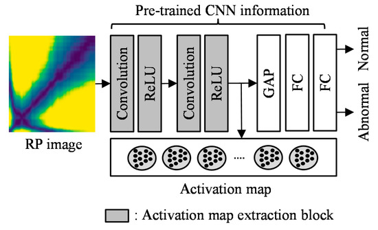
Figure 13.
CNN architecture for unsupervised feature extraction.
2.3. Health Indicator with Mahalanobis Distance
Mahalanobis distance (MD) is a distance measure between multivariate data points that considers the correlation of the multi-variates. An MD value is calculated using the normalized value of multi-variates and the covariance [28]. A health indicator (HI) is defined using MD to assess the health condition of the welding electrode tip.
where a(i) is the absolute value of the flattened vector of the activation maps for the ith weld point; μ is the average value of the flattened vector of the activation maps of the weld points during the training process; and Σ is the covariance of the activation maps of the weld points during the training process. When the average value and covariance are calculated using training RP images, MD values can be computed using individual test RP images acquired during the spot welding process.
3. Case Study
This section presents a case study to determine when degraded electrodes in a resistance spot welding system should be replaced to ensure the quality of welds in a product. Section 3.1 describes the experimental setup. Section 3.2 evaluates the performance of the proposed methodology using the testbed data.
3.1. Experimental Setup
The spot welding testbed is shown in Figure 14. The testbed was manufactured by Chowel (Ansan-si, Korea) and Hubis (Daejeon, Korea). The spot welder of the testbed was controlled by the Welcom-1000 software. To accelerate the degradation of the welding electrode tips, the electrical current used for welding was intentionally increased above that of normal conditions. The waveforms and images were recorded for individual spot welding, including dynamic resistance, pressure, current, and images of the upper and lower welding electrodes. A single set of data was collected every 2.2 s. The sampling rate was 50 kHz. A dataset was collected until 100 weld points were obtained. Then, the degraded welding electrode was replaced with a new one. Five welding electrodes were tested. Therefore, five datasets were generated for the five welding electrode tests.
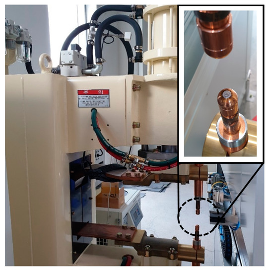
Figure 14.
Spot welding testbed.
Another dataset was collected until 500 weld points were obtained. For this particular dataset, the experiment was terminated when the symptoms of failure were observed by domain experts in the field. As shown in Figure 15, the maximum value and the slope of the dynamic resistance decreased from one to 375 weld points. After 375 weld points, the dynamic resistance waveform shape changed drastically. The database collected from the accelerated testing of the welding electrodes is summarized in Table 4.
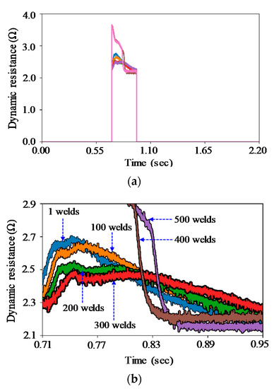
Figure 15.
Dynamic resistance data by weld number: (a) full view and (b) magnified view between 0.71 s and 0.95 s.
Table 4.
Database collected from the accelerated testing of welding electrodes.
CNN was trained using an Adam optimizer [29]. The learning rate was 0.001, while the batch size was 16. The number of training images was 500, while the number of test images was 1000. The shape of the activation maps was 12 × 1. The activation maps were used to calculate the health indicator using MD. The graphical processing unit was an NVIDIA Geforce Titan V GPU. Python 3.6 and TensorFlow 1.8 were used on the Linux operating system (Ubuntu 18.04).
3.2. Results and Discussion
Images with the size of 600 pixels by 600 pixels were obtained by converting the dynamic resistance waveforms using the proposed RP. Representative examples are shown in Figure 16. The yellow area decreases as the weld points increase, as presented from Figure 16a–d. The yellow area increases as the maximum value of dynamic resistance increases. The blue line increases as the slope of dynamic resistance increases. Therefore, the proposed RP can present multiple features of dynamic resistance in a single image. Figure 16e,f shows the images after failure. The domain experts determined that the welding electrode should be replaced after 375 welds were conducted.
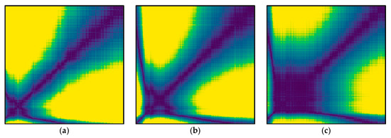
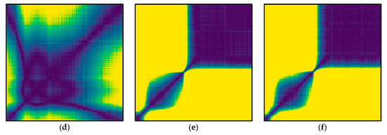
Figure 16.
Proposed RP images of dynamic resistance after (a) one, (b) 100, (c) 200, (d) 300, (e) 400, and (f) 500 spot welding instances.
Health indicators (HIs) were compared using the images from the original and proposed RP, as shown in Figure 17. As presented in Figure 17a, the HI curve using the original RP showed a gradual increase until 375 welds were conducted; whereas, the HI value decreased after 375 welds were conducted. As presented in Figure 17b, the HI curve using the proposed RP presented a monotonic increase even after 360 weld points. Therefore, it was concluded that the proposed RP outperforms the original RP. The instant spatter phenomenon that occurred after 420 weld points was also captured by the HI curve.
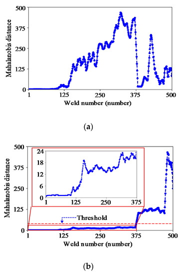
Figure 17.
Proposed degradation curve of a welding electrode: (a) original RP and (b) proposed RP.
A peel test was conducted to provide direct evidence of failure. The peel test results are shown in Figure 18. The replacement point was determined to be approximately 353 weld points when the nugget size was below 5 mm. When the HI value was 20, the replacement point for the welding electrode tip corresponded to 360 weld points.
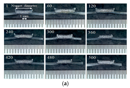

Figure 18.
Peel test result by weld number: (a) cross sectional view of welding and (b) nugget diameter versus weld number.
To compare the performance of the proposed methodology with prior methods, handcrafted features were employed. The knowledge-based features consisted of the resistance at each half-cycle peak, maximum resistance, time of maximum resistance, positive resistance slope, negative resistance slope, mean resistance value, final resistance value, and standard deviation of the resistance [1,13,14]. In this study, either five or eight features were incorporated. Depending on the number of features, the degradation curves fluctuated, as shown in Figure 19. It was difficult to decide a particular threshold value since the HI curve was not monotonic. The results showed that the proposed RP-based approach outperformed the handcrafted, feature-based approach.
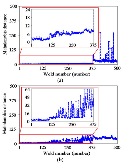
Figure 19.
Feature-based degradation curve of a welding electrode: (a) five features and (b) eight features.
4. Conclusions
This paper presented a methodology to determine the replacement cycle of welding electrode tips using dynamic resistance data. The proposed methodology consists of three key steps: (1) waveform imaging; (2) unsupervised feature extraction; and (3) welding electrode condition assessment. First, 1D waveforms are converted into 2D images. This study proposed a novel imaging method that is modified from the original recurrence plot (RP) imaging method. The proposed RP imaging method was devised to improve sensitivity to weak changes in a nonstationary signal and to enhance the method’s robustness to external noise. Convolutional neural networks (CNNs) were used for unsupervised feature engineering. A pre-trained CNN was used to develop activation maps. Finally, a health indicator that assesses the condition of welding electrode tips was built using Mahalanobis distance (MD), which was calculated from the outputs of the activation maps.
The performance of the proposed RP was evaluated with two different types of waveform signals, including (1) the positive half cycle of the sinusoidal waveforms and (2) the waveforms that emulate the evolution of dynamic resistance during resistance spot welding. From visual inspection and quantitative evaluation, it was found that the proposed RP is sensitive to amplitude changes of the simulated waveform, while being robust to random noise. For example, with the simulated dynamic resistance waveforms, the increase of the yellow area’s ratio between f1(x) and f3(x) using the proposed RP was 21.75%; whereas, the increase using the original RP was only 45.06%. The proposed RP showed double the sensitivity of the original RP.
A case study was conducted with a testbed using a real spot welding machine. From the case study, it was concluded that the methodology with the proposed RP imaging method outperformed the original RP imaging method and outperformed handcrafted, feature-based approaches. The results of presented methodology demonstrated the feasibility of monitoring a welding electrode condition in real time. It is anticipated that this study will help to determine the optimal replacement interval of electrode tips in spot welding systems subjected to variable working conditions.
The proposed methodology has two limitations. First, the threshold of N in the proposed RP should be determined by the user. Second, a criterion that determines the failure of welding electrodes was chosen based on the data from a single experiment. A statistical test method such as the sequential probability ratio test (SPRT) may help select the criterion. In the future, the proposed method will be further evaluated with data from real spot welding machines in the field.
Author Contributions
Conceptualization, H.O.; methodology, W.J.; validation, D.H.Y. and Y.G.K.; resources, J.P.Y. and J.H.P.; writing—original draft preparation, W.J.; writing—review and editing, H.O.; supervision, H.O. All authors have read and agreed to the published version of the manuscript.
Funding
This research was supported in part by Korea Ministry of Planning and Budget Foundation through Korea Institute of Industrial Technology (Project Number: JH190001) and in part by the Cross-Ministry Giga KOREA Project grant funded by the Korea Government (MSIT), (GK20P0700, 5G-Based Production/Logistics Service and Machine-Learning Platform Development for Cloud Manufacturing).
Conflicts of Interest
The authors declare no conflict of interest.
References
- Li, W. Monitoring and Diagnosis of Resistance Spot Welding Process. Ph.D. Thesis, University of Michigan, Ann Arbor, MI, USA, 1999. [Google Scholar]
- Ma, Y.; Wu, P.; Xuan, C.; Zhang, Y.; Su, H. Review on techniques for on-line monitoring of resistance spot welding process. Adv. Mater. Sci. Eng. 2013, 2013, 1–6. [Google Scholar] [CrossRef]
- Zapata, J.; Vilar, R.; Ruiz, R. Performance evaluation of an automatic inspection system of weld defects in radiographic images based on neuro-classifiers. Expert Syst. Appl. 2011, 38, 8812–8824. [Google Scholar] [CrossRef]
- Peng, J.; Fukumoto, S.; Brown, L.; Zhou, N. Image analysis of electrode degradation in resistance spot welding of aluminum. Sci. Technol. Weld. Join. 2004, 9, 331–336. [Google Scholar] [CrossRef]
- Simoncic, S.; Podrzaj, P. Image-based electrode tip displacement in resistance spot welding. Meas. Sci. Technol. 2012, 23, 065401. [Google Scholar] [CrossRef]
- You, D.; Gao, X.; Katayama, S. WPD-PCA-based laser welding process monitoring and defects diagnosis by using FNN and SVM. IEEE Trans. Ind. Electron. 2015, 62, 628–636. [Google Scholar] [CrossRef]
- Martín, Ó.; Pereda, M.; Santos, J.I.; Galán, J.M. Assessment of resistance spot welding quality based on ultrasonic testing and tree-based techniques. J. Mater. Process. Technol. 2014, 214, 2478–2487. [Google Scholar] [CrossRef]
- Luo, Y.; Rui, W.; Xie, X.; Zhu, Y. Study on the nugget growth in single-phase AC resistance spot welding based on the calculation of dynamic resistance. J. Mater. Process. Technol. 2016, 229, 492–500. [Google Scholar] [CrossRef]
- Tseng, K.H.; Chuang, K.J. Monitoring nugget size of micro resistance spot welding (Micro RSW) using electrode displacement-time curve. Adv. Mater. Res. 2012, 463–464, 107–111. [Google Scholar] [CrossRef]
- Ji, C.T.; Zhou, Y. Dynamic electrode force and displacement in resistance spot welding of aluminum. J. Manuf. Sci. Eng. 2004, 126, 605–610. [Google Scholar] [CrossRef]
- Dickinson, D.W.; Franklin, J.E.; Stanya, A. Characterization of spot welding behavior by dynamic electrical parameter monitoring. Weld. J. 1980, 59, 170–176. [Google Scholar]
- Hao, M.; Osman, K.A.; Boomer, D.R.; Newton, C.J. Developments in characterization of resistance spot welding of aluminum. Weld. J. 1996, 75, 1–8. [Google Scholar]
- Xing, B.; Xiao, Y.; Qin, Q.H.; Cui, H. Quality assessment of resistance spot welding process based on dynamic resistance signal and random forest based. Int. J. Adv. Manuf. Technol. 2018, 94, 327–339. [Google Scholar] [CrossRef]
- Wan, X.; Wang, Y.; Zhao, D.; Huang, Y.; Yin, Z. Weld quality monitoring research in small scale resistance spot welding by dynamic resistance and neural network. Measurement 2017, 99, 120–127. [Google Scholar] [CrossRef]
- Wan, X.; Wang, Y.; Zhao, D. Quality monitoring based on dynamic resistance and principal component analysis in small scale resistance spot welding process. Int. J. Adv. Manuf. Technol. 2016, 86, 3443–3451. [Google Scholar] [CrossRef]
- Wan, X.; Wang, Y.; Zhao, D.; Huang, Y. A comparison of two types of neural network for weld quality prediction in small scale resistance spot welding. Mech. Syst. Signal Process. 2017, 93, 634–644. [Google Scholar] [CrossRef]
- Randall, R.B. Vibration-Based Condition Monitoring, 1st ed.; Wiley: New Delhi, India, 2011. [Google Scholar]
- Marwan, N.; Carmen Romano, M.; Thiel, M.; Kurths, J. Recurrence plots for the analysis of complex systems. Phys. Rep. 2007, 438, 237–329. [Google Scholar] [CrossRef]
- Eckmann, J.P.; Kamphorst, S.O.; Ruelle, D. Recurrence plots of dynamical systems. Europhys. Lett. 1987, 4, 973–977. [Google Scholar] [CrossRef]
- Nichols, J.M.; Trickey, S.T.; Seaver, M. Damage detection using multivariate recurrence quantification analysis. Mech. Syst. Signal Process. 2006, 20, 421–437. [Google Scholar] [CrossRef]
- Manetti, C.; Giuliani, A.; Ceruso, M.-A.; Webber Charles, L.; Zbilut, J.P. Recurrence analysis of hydration effects on nonlinear protein dynamics: Multiplicative scaling and additive processes. Phys. Lett. A 2001, 281, 317–323. [Google Scholar] [CrossRef]
- Marwan, N.; Wessel, N.; Meyerfeldt, U.; Schirdewan, A.; Kurths, J. Recurrence-plot-based measures of complexity and their application to heart-rate-variability data. Phys. Rev. E 2002, 66, 026702. [Google Scholar] [CrossRef]
- Simonyan, K.; Zisserman, A. Very deep convolutional networks for large-scale image recognition. In Proceedings of the 3rd International Conference on Learning Representations, San Diego, CA, USA, 7–9 May 2015. [Google Scholar]
- He, K.; Zhang, X.; Ren, S.; Sun, J. Deep residual learning for image recognition. In Proceedings of the IEEE Conference on Computer Vision and Pattern Recognition, Las Vegas, NV, USA, 27–30 June 2016. [Google Scholar]
- Guerin, J.; Gibaru, O.; Thiery, S.; Nyiri, E. CNN features are also great at unsupervised classification. In Proceedings of the 4th International Conference on Artificial Intelligence and Applications, Melbourne, Australia, 17–18 February 2018. [Google Scholar]
- Girish, D.; Singh, V.; Ralescu, A. Unsupervised clustering based understanding of CNN. In Proceedings of the IEEE Conference on Computer Vision and Pattern Recognition Workshops, Long Beach, CA, USA, 16–20 June 2019; pp. 9–11. [Google Scholar]
- LeCun, Y.; Bottou, L.; Bengio, Y.; Haffner, P. Gradient-based learning applied to document recognition. Proc. IEEE 1998, 86, 2278–2324. [Google Scholar] [CrossRef]
- Mahalanobis, P.C. On the generalized distance in statistics. Proc. Natl. Inst. Sci. India 1936, 2, 49–55. [Google Scholar]
- Kingma, D.P.; Ba, J. Adam: A method for stochastic optimization. In Proceedings of the 3rd International Conference for Learning Representations, San Diego, CA, USA, 7–9 May 2015. [Google Scholar]
© 2020 by the authors. Licensee MDPI, Basel, Switzerland. This article is an open access article distributed under the terms and conditions of the Creative Commons Attribution (CC BY) license (http://creativecommons.org/licenses/by/4.0/).