Featured Application
Indoor and outdoor air pollution has reached a hazardous level. Therefore, there is an urgent necessity to monitor and control air quality to protect human health. In this scenario, research in the field of sensors and advanced sensing techniques plays a strategic role. This work is a review of the state-of-the-art and future possibilities of FES aiming at providing a starting point and aid for researchers interested in working in this promising field of advanced sensing.
Abstract
Fluctuation-enhanced sensing (FES) is a very powerful odor and gas sensing technique and as such it can play a fundamental role in the control of environments and, therefore, in the protection of health. For this reason, we conduct a comprehensive survey on the state-of-the-art of the FES technique, highlighting potentials and limits. Particular attention is paid to the dedicated instrumentation necessary for the application of the FES technique and also in this case limits and possible future developments are highlighted. In particular, we address resolution, measurement speed, reproducibility, memory, noise, and other problems such as the influence of humidity. A number of techniques and guidelines are proposed to overcome these problems. Circuit solutions are also discussed.
1. Introduction: Gas Sensing for Health Protection
The problem of air pollution is now being actively investigated all over the world [1,2,3,4]. Due to its influences both on health and on global economy, air pollution is the foremost concern especially in modern cities [5], but also for fragile and highly sensitive ecosystems that are increasingly affected by upwind urban areas and industrial activities [6]. Due to the increase in population density, with consequent increase in means of transport and the rising of global warming leading to the abrupt climate changes, air pollution has reached a hazardous level. Therefore, there is an urgent necessity to monitor and control the pollution to protect human beings, animal health, and plant life. Great efforts have been made by environmental protection agencies and governments to reduce the influences of the air pollution upon communities [7,8] and recent advancements in the field of wireless communication technology and digital electronics have raised a new paradigm for air pollution monitoring [9,10], which takes advantage of communication and mobile progresses [11,12].
However, the problem of air-pollution does not concern only outdoor air; indoor environment pollution, in fact, could be even more dangerous than the former for the health [13]. Indeed, indoor air may contain a wide variety of volatile organic compounds (VOC) that may cause, in case of exposure to them, mucous irritation, neurotoxic effects, and nonspecific reactions [14,15,16]. Several monitoring techniques are being developed for the study of indoor environment, such as gas distribution mapping (GDM), which can be used to evaluate the efficiency of environmental control systems and identify pollutant sources [17]. Obviously, a fundamental role is played by the quality of the sensors used, in terms of sensitivity, selectivity, and fast response. The classical Taguchi-type semiconductor gas sensor bases its principle of operation on the change of its resistance as the gas to be sensed is adsorbed onto the sensor surface [18] and it represents a low cost solution.
Metal oxides are the most commonly used sensing materials [19]. Nanostructured materials offer some distinctive advantages in this area, such as small grain size, controlled growth of morphology and heterojunction effect provided by compositing techniques, making them good candidates for CO2 gas sensors [20]. The porous structure of one class of these materials, by offering a high surface area, increases the sensitivity of the gas sensors [21,22]. Not only the high surface area, but also the actual nanostructure plays a key role for sensitivity enhancement of nanostructured materials [23]. Sensitivity can also be improved by doping the oxide materials [19,24].
The alarming rise of indoor pollution has promoted, thanks to appealing physical, chemical, optical, and electronic properties of new materials, increasing effort in advanced sensing materials. The state-of-art gas-sensing nanomaterials and their future perspectives are well-documented and summarized in [25].
However, improvements in all the above-mentioned directions cannot be achieved without further research on the mechanisms of the proceeding reactions and phenomena and on other impacting factors. Indeed, much work is still required for the application of new materials in the real life devices [26].
To improve the performance of gas sensors, in parallel with the research in the field of new materials, it is possible to explore new advanced sensing techniques, even exploiting standard sensors. For example, chemical selectivity of semiconductor gas sensors can be boosted by operating an array of sensors, each of them having different sensitivity to different gases (the so called Electronic Nose) [27]. A pattern recognition method must be employed to analyze the output of the sensors array [28] and machine learning technique can also be used [29]. Chemical selectivity can also be improved by investigating the dynamic response of temperature modulated sensors [30].
However, almost all of the investigated gas sensors still suffer from lack of selectivity. Coupling smart gas sensors with artificial intelligence algorithms could be a solution to empower conventional gas sensing technologies and increase accuracy in gas detection [31].
In the next sections we review a powerful sensing technique, which allows to reach sensitivities orders of magnitude higher than that of classical sensing methods, even when compared to standard commercial electronic noses: fluctuation-enhanced sensing (FES). At first, we review the basics of FES and the idea from which it takes its origins, then we review the evolution and the state-of-the-art of FES, together with the most common implementation issue including the dedicated instrumentation required for reaching the highest sensitivity. Prospects and future developments will also be discussed.
2. Fluctuation Enhanced Sensing: A Powerful Sensing Technique
The conception and development of the fluctuation-enhanced sensing (FES) [32] stems from the observation that, even in the field of sensing, the microscopic, random fluctuation phenomena in physical systems are rich sources of information.
Physical and chemical sensing techniques usually involve the measurement of the value of a physical quantity in the detector/sensor. FES was first proposed and developed for chemical and gas sensing and, unlike traditional sensing methods, it takes advantage of the fact the sensed agent changes the statistics of the neural output (a pulse noise) thus acting in a way completely analogous to biological sensing. It is important to underline that in FES it is the noise that carries the sensory useful information. Note that in the past, FES has been used for the measurement of some physical quantities, but the knowledge and technologies available made the application of the technique somewhat complicated.
For example, by measuring Johnson noise voltage of resistors it is possible to estimate the temperature [33].
Figure 1 shows the principle on which the usual Johnson voltage noise thermometry is based (Figure 1b), compared with classical resistor thermometry (Figure 1a) and with the application of FES (Figure 1b and 1c combined together). To measure the temperature with a classic resistor, the law of variation of the resistance with temperature R(T) must be known and, furthermore, to measure the actual value of the resistance a DC bias current is required. This current, however, heats up the resistor thus causing errors in the measurement of T. Although for the conventional Johnson-noise thermometry the R(T) function is not needed, the problem of measuring the resistance value R still exists, unless its value is independent of the temperature.
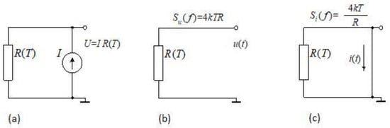
Figure 1.
(a) Resistor thermometer; the R(T) function and R value must be known and a biasing DC current I that, by unavoidably heating the thermometer causes error, is needed; (b) the usual Johnson-noise thermometry: SU is the power spectral density of the voltage fluctuations across the resistor, k is the Boltzmann constant, and T is the absolute temperature. Differently from the resistor thermometer, the R(T) function is not needed but the resistance value R must be known; (c) fluctuation-enhanced absolute thermometry based on Johnson noise and first principles: the Johnson voltage and current noise are measured (circuits b and c). The combination of the two measurements provides both the absolute temperature T and the resistance R. No heating occurs and no preliminary knowledge is needed if accurate current and voltage noise measurement systems are available.
However, if the measurement of the voltage noise (b) and of the current noise (c) are combined, we can obtain absolute thermometry based on Johnson noise and first principles and this can be regarded as evidence of the power of FES. Indeed, when both Johnson voltage noise and current noise are measured, we obtain two separate equations. The solution of such a system allows to derive both the absolute temperature T and the resistance R:
In Equation (1) Su and Si are the power spectral densities (PSD) of the voltage and current fluctuations, respectively, and k is the Boltzmann constant. Compared to the other measurement methods, it must be stressed that in this case no heating occurs and only precise current and voltage measurements are needed. This consideration also indicates that FES, regardless of its simplicity or cheapness, is a very powerful tool.
In this paper we want to focus on fluctuation-enhanced sensing of gases and odors, being a topic of great current interest for the control of environments and therefore for the protection of health. To understand the principle and the reason for resorting to FES as gas sensing technique, let us start from the observation that classical gas sensing methods are many orders of magnitude less sensitive than the best gas sensing systems we have in nature: dog noses (or even that of humans). It is therefore fundamental, as a first step, to understand how biological noses work. The operating principle of biological noses is shown in Figure 2. They contain a large array of olfactory neurons that communicate stochastic voltage spikes to the brain. When odor molecules are adsorbed by a quantity of neurons, the statistical properties of these stochastic spikes change. The brain decodes the changes in statistics and matches the result with an odor database in memory.
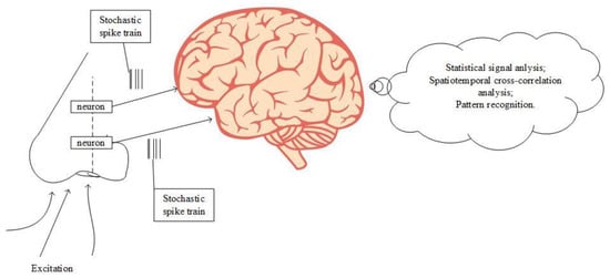
Figure 2.
Operating mode of fluctuation-enhanced odor sensing by biological noses.
The first step is common to the classical sensing method: the value of a physical quantity in the sensing medium is measured (for example the output voltage of a chemical sensor). In FES, however, the microscopic spontaneous fluctuations, due to the dynamically changing molecular-level interactions between the odor molecules and the sensing media, superimposed to the average value taken into consideration in classical sensing, are strongly amplified (typically 1–100,000 times) and the statistical properties of these fluctuations are analyzed, with an approach that is somewhat similar to the operation of a biological nose.
Note that the chemical signature of the odor is contained right in the fluctuations. The results of the analysis are compared with a statistical pattern database to identify the odor. Since, unlike the classic sensing methods in which a measurement of the average values of the electrical signals (voltage or current) is carried out, the biological sensing exploits the fluctuations of the signals to reach much higher sensitivity, the sensing technique we discuss, which operates on the same principle, has been named “fluctuation-enhanced” sensing [34,35,36,37,38,39,40] or FES. Even if the FES method does not reach now the sensitivity level of a dog nose in commercial or proto-type gas sensors, its principle mimics the sense of smell. Moreover, the sensitivity of the FES method can be sharply improved by using a smaller volume of the sensing layer as discussed in Section 4. Indeed, tiny gas sensing layers, made of nano-particle materials, tend to the size of smell cells in biological objects, characterized by lower detection threshold levels.
3. Fluctuation-Enhanced Gas Sensing: A Brief Historical Overview
Most chemical sensors produce a single output, such as, for example, the steady-state value of the resistance of a Taguchi sensor [18], or the steady-state current value of a MOS sensor. To generate a separate pattern corresponding to different chemical compositions, like in the case of electronic noses, a number (6–40) of different types of sensors are needed, which makes the system expensive and unreliable for practical applications. On the other hand, fluctuation-enhanced sensing (FES), as illustrated in Figure 3, by analyzing the fluctuations rather than the DC value, is capable of generating complex patterns even by starting from a single sensor [41,42,43,44,45,46,47,48] and this fact represents a great advantage with respect to other more conventional sensing techniques.
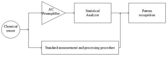
Figure 3.
Schematic diagram for fluctuation-enhanced chemical sensing.
When applying FES, instead of using the mean value (time average) of the sensor signal, the small stochastic fluctuations around the mean value are amplified and statistically analyzed. Resistive film sensors, due to their grainy structure, present electronic resistance fluctuations several orders of magnitude higher if compared to the case of single crystalline materials, and these fluctuations are strongly influenced by the random diffusion dynamics of agents in the proximity of inter-grain junctions and by adsorption-desorption noise. Stochastic analytical tools are used to generate a one-dimensional or two-dimensional pattern from the time fluctuations and pattern recognition tools are employed for their analysis.
The origin of FES dates back to more than two decades ago but the name “fluctuation-enhanced sensing” was coined by John Audia (SPAWAR, US Navy) in 2001. The solution of employing electrical noise (spontaneous fluctuations) to identify chemical agents was first proposed by Bruschi and coworkers [41,42] in 1994–1995 by showing the high sensitivity of conductance noise spectra of conducting polymers to the ambient gas composition. Gottwald and coworkers [43], a few years later (1997), also published similar observations about the conductance noise spectra of semiconductor resistors with non-passivated surfaces. In 1998, Kish and coworkers designed the first FES system capable of quantitative analysis of gas mixtures and conducted mathematical analysis about the limits and the sensor number requirement versus the number of agents [44,45,46]. In [45] it was demonstrated the effectiveness of the sampling-and-hold technique as a way of “freezing the odor” (see Section 6.2.1) in a Taguchi sensor and later a more extensive analysis on the subject was published by Solis et al. [47]. In 2001, Smulko et al. were the first ones to use higher-order statistics to enhance the extracted information from the stochastic signal component [48] and they confirmed the robustness of their approach with successive works [49,50,51]. Hoel et al. showed FES via invasion noise effects at room temperature in nanoparticle films [52]. Schmera and coworkers analyzed the situation of Surface Acoustic Wave (SAW) sensors and predicted the FES spectrum for SAW and MOS sensors with surface diffusion [53,54]. Commercial-Off-The-Shelf (COTS) sensors exposed to environmental pollutants and gas combinations were also studied [55,56,57]. In nanoparticle sensors with a temperature gradient, the possibility of using the noise of the thermoelectric voltage for FES was demonstrated [51]. Ederth et al. analyzed the sensitivity enhancement in the FES mode and compared it to the classical mode in nanoparticle sensors and found an enhancement of a factor of 300 [58]. Gomri et al. [59,60] published FES theories for the cases of adsorption-desorption noise and chemisorption-induced noise and, recently, in [61] Gomri et al. theoretically demonstrated that the product of frequency by the power spectral density of the gas sensing layer resistance fluctuations often has a maximum which is characteristic of the gas, thus providing a valid method for gas classification. They experimentally confirmed this property in the case of the detection of NO2 and O3 using a WO3 sensing layer. Huang et al. explored the possibility of using FES in electronic tongues [62]. When carbon nanotubes gained importance in the field of sensors and there was a strong growth in their applications, the FES technique was also applied to increase the sensitivity of these materials [63,64,65,66] and also the noise characteristics of graphene, which shows, with respect to the vast majority of ordinary semiconductors, a peculiar behavior of the flicker noise power spectral density as a function of the charge carrier density, have been investigated for possible application in FES [67]. FES has also been applied to amperometric gas sensor measurements [68,69].
In order to take advantage of FES potentialities, special low-noise measurement hardware and software to acquire data and perform analysis are required. Although an in-depth discussion on this topic will be made in Section 6, here we briefly emphasize that the FES devices have followed the evolution of electronics, therefore several solutions have been presented in literature, such as, for example, a small, USB-powered device [70], tested on Taguchi and carbon nanotube based gas sensors, and a complete mixed-signal system [71]. Today we live in the era of the Internet of Things (IoT), which provides opportunity to continuously monitor different aspects of our lives in a cost-effective way. Since FES is a promising method to increase the selectivity and sensitivity of the sensors, an attempt to realize a complete wireless sensor node system based on Wi-Fi communication has also been made [72] which is a significant step toward the possibility of using fluctuation-based sensing methods in everyday life.
4. Fundamental FES Resolution Limits
4.1. On the Sensitivity and Selectivity
Microscopic fluctuations perturbations require very small energy, so their statistics in a system carry a lot of information about the system itself. On the other hand, while classical sensing techniques use as information a single value obtained as mean value of the sensor signal, in the case of FES the related statistical distribution functions are data arrays, and thus they can contain orders of magnitude more information.
The underlying physical mechanism behind the enhanced sensitivity is the temporal fluctuations of the agent’s or its fragment’s concentration at various points of the sensor volume where the sensitivity of the resistivity against the agent is different. This effect generates stochastic fluctuations of the resistance and, hence, of the sensor voltage when it is biased with a DC current. The voltage fluctuations can be extracted (by removing the mean value by AC coupling) and strongly amplified. Sensitivity enhancement by several orders of magnitude was demonstrated by Kish and coworkers [56] in Taguchi sensors and by Ederth and coworkers [58] in nanoparticle films.
Significantly increased selectivity can be expected depending on the type of sensor and types of available FES “fingerprints”. We define the selectivity enhancement by the factor specifying how many classical sensors a single fluctuation-enhanced sensor can replace. When using power density spectra, the theoretical upper limit of selectivity enhancement is equal to the number of spectral lines that is, typically, about 10,000. However, when the elementary fluctuations are random-telegraph signals (RTSs) the underlying elementary spectra are Lorentzians [73,74] and the situation is less favorable because their spectra strongly overlap. Consequently, experiments with COTS sensors indicate that the response of spectral lines against agent variations is often not independent. In a simple experimental demonstration with COTS sensors, a selectivity enhancement of six was easily reachable [38]. However, nanosensor implementation may be able to use all the spectral lines more independently. As both the FES signal in macroscopic sensors and the natural conductance fluctuations of the resistive sensors usually show 1/f-like spectra [73,74], the lower the inherent 1/f noise strength in the sensor the cleaner the sensory signal. An interesting analysis can be made if we suppose that we shrink the sensor size so much that the different agents probe different RTS signals. Then principles for 1/f noise generation [75] indicate that one can resolve at most a few Lorentzian components in a frequency decade. Supposing six decades of frequency, the maximal selectivity enhancement would be around 18, supposing three fluctuators/decade.
With bispectra [48,49,50], the potential for selectivity increase is even greater because bispectra are two-dimensional data arrays. In the case of 10,000 spectral lines, as mentioned above, the theoretical upper limit of selectivity increase is 100 million, but in the Lorentzian fluctuator limit that number is again radically reduced. Bispectra sense only the non-Gaussian part of the sensor signal, and for the utilization of the full advantages of bispectra it seems necessary to build the sensor within the submicron characteristic size range in order to utilize elementary microscopic switching events as non-Gaussian components. Moreover, the sixfold symmetry of the bispectrum function yields a further reduction of information by roughly a factor six. Using the above-mentioned estimation with three Lorentzian fluctuators/decade, over six decades of frequency, the selectivity enhancement would be around 50. It should be noted that this enhancement is independent from the spectral enhancement discussed above because bispectra probe the non-Gaussian components [73].
4.2. Information Channel Capacity in Classical (Deterministic) Gas Sensors
Kish and coworkers have shown [73] that in the case of homogeneous probing current density in the sensor and if the sensor resistance fluctuations in the reference gas have 1/f spectrum, by using Shannon’s formula of information channel capacity in analog channels, classical resistive sensors have the following upper limit of information flow rate:
where tm is the measurement time window, R and R0 are the resistance response in the test gas and in the reference gas, respectively, V is the volume of the sensor film, AS is the surface of the sensor film, and d is its thickness. The factor A characterizes the strength of 1/f noise of the conductance noise spectrum [73] in the specific sensor by the simplified Hooge formula:
where U is the DC voltage drop across the resistive sensor and f is the frequency.
According to Equation (2), in the practical (1/f-noise-dominated) limit and at fixed measurement time and film thickness, the larger the surface of the classical resistive sensor the greater the information channel capacity. However, in the limit of a sufficiently large agent concentration, the saturation time is controlled by the underlying diffusion processes taking place through the thickness of the film; therefore, in this case, the shortest measurement time is also controlled by diffusion according to
where D is the diffusion coefficient of the agent and/or its fragments through the film. Therefore, the thinner and larger the film, the greater the information channel capacity. This fact indicates that, in classical films, small thickness and large surface are preferable, with the thickness being the dominant control parameter.
4.3. Information Channel Capacity in Fluctuation-Enhanced (Stochastic) Sensing
Current understanding of related fluctuations implies that the spectrum S(f) is the superposition of elementary Lorentzian spectra sj(f). Physically, each of such a Lorentzian fluctuators has an underlying exponential relaxation process with a single time constant τj determined by microphysical parameters:
where sj(f) is the spectrum originating from the j-th fluctuator, Cj is its strength, and τj is its time constant.
Suppose the power density spectrum of the resistance fluctuations in a FES sensor has K different frequency ranges, in which the dependence of the response on the concentration of the chemical species is different from the response in the other ranges, one can write [43,44,45]:
where ΔS(fi) is the change of the power density spectrum of resistance fluctuations at the i-th characteristic frequency band, and the Ai,j quantities are calibration constants in the linear response limit. Thus, a single sensor is able to provide a set of independent equations to determine the gas composition around the sensor. The number K of different applicable frequency ranges has to be greater than or equal to the number N of chemical species, i.e., K ≥ N. To meet the ideally required requirements, the sensors should exhibit linear responses. Unfortunately, in [55] it has been shown that commercial Taguchi sensors do not satisfy such a condition (see Figure 4, which has been reported here for the sake of clarity). It is however reasonable to speculate that nanoscale devices may meet this requirement because of the linear superposition of elementary fluctuations.
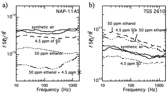
Figure 4.
Experimental proof that the response in Taguchi sensors is not additive (nonlinear) [55]. Both in the case of the sensor NAP-11AS (a) and of the sensor TGS 2610 (b), the response to a mixture of two chemicals (ethanol and S2O) is not the sum of the responses obtained when each chemical is alone in the test chamber.
In [73], the information channel capacity of power density spectrum based FES was estimated by assuming equal frequency bands and supposing that the relative error of the spectrum is much less than unity, then the information channel capacity (roughly) scales as:
where tw is the duration (time window) of a single data sequence (for a single Fourier transformation), tm is the total measurement time (the elementary power spectra are averaged over that), and fs is the sampling frequency. It is supposed that the FES measurement starts after the sensor reached a stationary state in the test gas and that tm is much longer than the time needed to reach the stationary state. Moreover, the condition of thin sensor film must be verified, just like in the case of the considerations for a classical sensor above.
In such a case, the most important conclusion of Equation (6) is that, in resistive FES applications, the sensor surface can be very small without limiting the performance (as large as enough Lorentzian fluctuators are present for each frequency band) because measurement time related statistical inaccuracies limit the information channel capacity, not the background noise.
In [73], similar conclusions are obtained for bispectrum based FES sensor systems.
5. Practical Sources of Errors
5.1. Turbulence and Convection
The flow of the carrier gas around the sensor can cause vortex/turbulence effects that are random in nature. Similarly, the convection of the hot air flying up from the heated sensors has random features. These phenomena contribute to the temperature fluctuations in heated sensors, which, in turn, cause resistance fluctuations because their resistance is usually strongly temperature dependent (they are typically semiconductors). These excess fluctuations are a nuisance because they interfere with the FES signals which are also fluctuations.
There is a method of operation, the “sampling-and-hold” (or “frozen-smell”) technique, that solves the above-mentioned problems (see details in Section 6.2.1 below).
5.2. Ambient Air, Unknown Agents, and Humidity
The FES spectral patterns of various gas compositions are learned by a classifier (a pattern recognizer such as a neural network) that will display the result of the analysis. However, strictly speaking, this approach only works for agents used in the training of the classifier, typically in a lab environment. When the FES system is used in the field, extra agents can be present. If they influence the FES spectra, they become a problem. Humidity can strongly vary and it typically has a major influence on the spectra. In this case, humidity must also be treated as an agent. Note that the human nose is using not only FES (via random neural signals) but also a large quantity of different types of olfactory neurons to compensate for these situations. Possibly, future chip technology can help with this problem by imitating biological smelling. Such a “visionary chip” would include a large number of diverse type and independent FES sensors integrated together with their signal processing units. The output signals of these units would be evaluated in a “spatio-temporal” fashion similarly to dog noses. Thus, not only the spectral features of the sensor signals would be evaluated but also transient, delay, and spatial and time correlation effects between the statistical responses of sensors. This would enrich the sensory information by surface and air diffusion responses similarly to biological noses.
5.3. Memory, Aging, Fabrication Variations
Noise is sensitive to the spatial correlations and their time variations in the molecular lattice of the sensor. This is the reason why FES is a much more sensitive and information rich tool than classical sensing based on resistivity changes. However, these enhancements come at a price: the noise may be too sensitive thus it may reflect on also memory, aging, and variations in fabrication. All these facts must be taken into the account and carefully monitored during applications. For marketable FES systems, the detailed study of aging and memory are yet to be done, similarly to many other sensing methods in the exploratory phase.
We underline that similar drawbacks limit both the FES method and the resistivity measurements. One important issue is time stability and unavoidable drifts of physical properties [65]. This difficulty is reduced by considering changes in the recorded physical properties, including statistical parameters. We have observed similar stability of noise measurements as for resistivity, at least in some of the tested gas sensing layers. The same remark is valid for repeatability of the measurement results delivered by noise phenomena. Data repeatability can be improved by cleansing, by using heating pulse, or UV-light irradiation.
5.4. Measurement Circuitry Problems: Noise, Bandwidth
Performing sensible low frequency noise measurements (LFNM) is never an easy task. The very instrumentation required for performing noise measurements introduce noise that may mask the noise coming from the Device Under Test (DUT), thus reducing the sensitivity that can be obtained. Since in the field of FES we are mainly interested in the low frequency noise generated by the DUT, it is generally the flicker component of the noise introduced by the instrumentation that sets the limit to the sensitivity that can be obtained. It must also be noted that LFNM measurement set-ups are extremely sensitive to interferences coming from the environment. Electro-magnetic interferences (EMI) at frequencies much higher than those one is interested in may translate into what could appear as additional low frequency noise components because of rectifying effects due to the active components in the measurement chain [76]. Even moderate air movement, in the immediate proximity of active components, as caused by unrestricted convection motion due to power dissipation, may result in apparent increase in the noise. Assuming that all causes of interferences are removed by proper shielding and positioning of the components, the ultimate sensitivity is set by the intrinsic noise introduced by the DUT bias systems, by the preamplifiers that detect and amplify the noise signal across the DUT and, possibly, by other auxiliary systems such as DUT temperature control systems. While standard instrumentation exists that can be used for laboratory set ups and even wafer level noise testing [77,78,79], depending on the DUT characteristics, dedicated instrumentation may be a better choice in order to maximize sensitivity [80] and, in the specific case of FES applications, portability. The most important problems to be faced and possible circuitry solutions will be discussed in Section 6.3.
6. Reducing Errors and Enhancing the Sensory Information Channel Capacity
6.1. Photonic Excitation
As we have mentioned before, conductance noise spectra are the superposition of over-damped Lorentzian spectra, which means no sharp peaks in the FES spectrum can be present. However, photonic excitations combined with FES measurements have the potential to increase the information content of measurements. With properly selected photon energies (wavelengths) some of the otherwise dormant states can be activated and they can produce a modified spectrum with new information.
UV Light Excitation Experiments and Results
Resistive gas sensors have limited selectivity and sensitivity, and therefore any cost-efficient method of gas sensing improvement is appreciated. Some gas sensing materials (e.g., WO3, TiO2, SnO2 nanowires, golden nanoparticle organically functionalized, carbon nanotubes, graphene) exhibit a photocatalytic effect. This effect can be easily induced by UV LEDs irradiating the gas sensing layer (Figure 5). Numerous papers are presenting the detailed results of gas sensing modulated by UV light applied to different gas sensing layers [81,82,83,84,85,86,87,88].
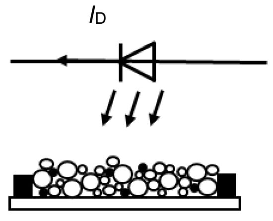
Figure 5.
Illustration of resistive gas sensing layer between the terminals (black rectangles) irradiated by UV LED biased by DC ID; the layer comprises of the grains of different size and dopants of noble metals (black dots) improving gas selectivity.
A series of low-cost UV LEDs, emitting UV light within wavelet range 250–355 nm is available on the market. Resistive gas sensing layer can be made on ceramic or silicon substrates and efficiently irradiated from different distances. Selected wavelengths of the UV light can modulate the physical properties of the gas sensing layer (e.g., DC resistance, low-frequency resistance fluctuations) [85]. It has been observed that changes of DC resistance induced by UV irradiation are independent of the changes of the recorded low-frequency noise [86]. Thus, both phenomena secure additional information about the ambient atmosphere and can be utilized to improve gas detection.
During FES experiments 1/f dependence with a plateau at selected corner frequencies, characteristic for an ambient gas and the wavelength of the applied UV LEDs, was observed. The intensity of the 1/f noise component was also informative and depended on gas concentration. The FES method was advantageous at low gas concentrations enhancing threshold gas detection. This effect was observed at an ambient atmosphere of different gases. It is a valuable result for practical applications, especially for medical diagnosis by exhaled breath analysis when deficient gas concentrations have to be detected. Moreover, faster response of the gas sensor was observed. This effect is rather evident because UV light was formerly applied to cleanse the sensor. UV irradiation replaced a heating pulse, commonly employed for fast sensor cleansing.
We should underline that a photocatalytic effect in gas sensing depends on a few independent factors:
- morphology of gas sensing layer, determining the depth of light penetration,
- irradiation intensity,
- the wavelengths of the UV light.
As we see (Figure 5), the gas sensing layer is a porous grainy material. The gas molecules can penetrate the pores of the whole gas sensing layer due to the diffusion process and change DC resistance or low-frequency resistance noise recorded between the terminals. The UV light penetrates only the thin part of the gas sensing layer. The depth of penetration depends on light wavelength, irradiated material and its morphology. We can assume that the depth of UV light penetration does not exceed a few µm [85]. Thus, the gas sensing layer can be modelled as two parallel resistors: an external one modulated by UV light and the inner one without this effect. It was observed that there is a threshold intensity of UV light when its further intensification does not induce the changes in the gas sensing layer. This effect is a result of a limited impact on the thin sensing layer only. The low-cost gas sensor in Figure 6, made of a mixture of graphene flakes (Graphene Supermarket UHC-NPD-100ML) and TiO2 nanoparticles (AEROXIDE® TiO2 P25) by painting and baking, has a thickness of about 100 µm, which is about 100 times more than the estimated depth of UV light penetration. Thus, UV light affects less than 1% of its porous and gas-sensitive volume.
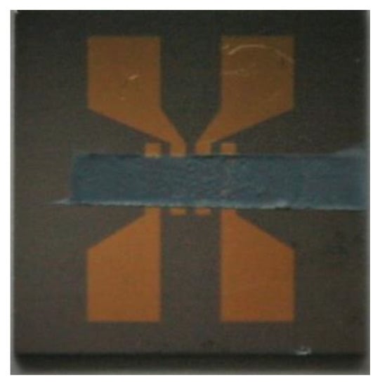
Figure 6.
Gas sensing layer comprising TiO2 nanoparticles and graphene flakes: photo of the sensor made by painting on a silicon substrate with four-point gold contacts.
The easiest way of increasing UV light modulation is to apply a thinner gas sensing layer. Moreover, a thinner layer will secure a faster gas response, which is very important for any practical application. The reduced thickness should result in other advantages, such as a lower price and lower energy consumption when operating at elevated temperatures. This result can be reached by spin coating technology, reducing the thickness of the sensing layer to the maximum of a few µm only and ensuring more even surface and more repeatable sensing properties.
Figure 7 presents results of 1/f noise power spectral density generated in the thick gas sensing layer shown in Figure 6. The sensor was irradiated by UV LED, having maximal optical power at the wavelength of 394 nm. Both materials (graphene flakes, TiO2 nanoparticles) are gas-sensitive and both exhibit the photocatalytic effect. The gas sensing layer has a very porous structure. A vivid change of power spectral density slope versus frequency was observed when UV light was applied. The intensified plateau of power spectral density was present about 10 Hz after irradiation. This effect can be explained by modulation of adsorption-desorption rate induced by UV light, making these processes faster and more intense. By increasing power of UV light (decreasing its wavelength), changing morphology of gas sensing layer (e.g., changing a graphene flakes/TiO2 ratio of wt%), and reducing a thickness of the gas sensing layer it is possible to strengthen this effect. More visible changes of plateau can be observed at lower operating temperatures when the energy of UV light had a greater impact on adsorption-desorption process.
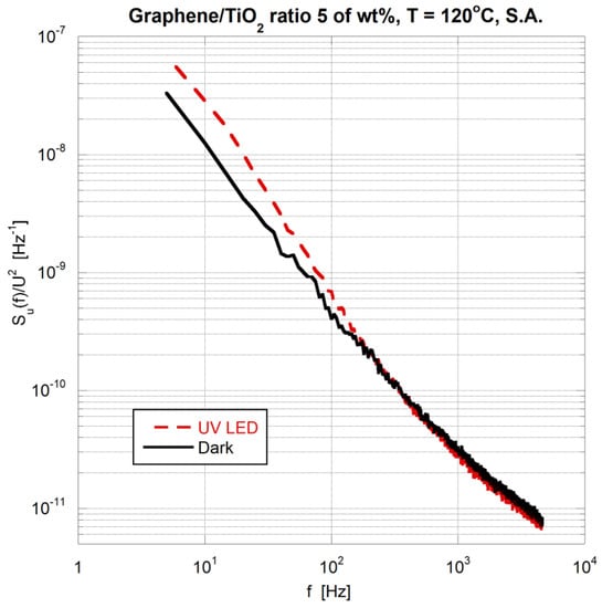
Figure 7.
Power spectral density Su(f) of voltage fluctuations across the gas sensor biased by DC voltage U and normalized to U2 versus frequency f; UV LED, type OSV4YL5451B, made by OptoSupply was irradiating the sensing layer with a graphene flakes/TiO2 ratio 5 of wt% (Figure 6) in the ambient atmosphere of synthetic air (S.A.) and at operating temperature T = 120 °C.
The FES method can be applied not only in resistive gas sensing layers. The back-gated FET gas sensors, utilizing graphene in a channel, exhibit 1/f spectra with a plateau at corner frequencies characteristic for selected ambient gases (e.g., chloroform, acetonitrile, methanol, ethanol) [87]. This result was observed when a single-layer-graphene was used on the channel. Then, low-frequency noise was related to individual events of gas molecules adsorption-desorption. A corner frequency of the observed plateau was stable for different specimens of the single-layer-graphene FET sensors at an ambient atmosphere of acetonitrile [87]. This result suggests that the FES method can be very selective and repeatable when the FET channel is a two-dimensional material of the same physical structure.
Another two-dimensional material, MoS2, was applied successfully for gas sensing using the FES method in back-gated FET sensors [89]. These experiments, however, require further in-depth studies to confirm the result for other gases and other materials.
We may suppose that in two-dimensional material the adsorbed molecules change the surface potential. Therefore, the observed low-frequency noise is modified by adsorption event more similarly for a given gas molecule than in a case of the porous gas sensing layer. In a bulk polycrystalline sensor, gas molecules modulate the potential barrier between the crystal grains, which have some size distribution. Any potential barrier modulation should depend on the size of the grains adsorbing the molecules. Thus, any 1/f noise change induced by the adsorbed molecule should be less characteristic in porous gas sensors, comprised of different grains, than in the FET sensor using two-dimensional material of repeatable structure in a channel. Moreover, we can suppose that the FES method in FET sensors can determine components of gas mixtures when each plateau in 1/f noise is related to the presence of different gas molecules. This conclusion is valuable for practical application when we have to consider gas mixtures and the effects of crossing gases.
Some experimental data suggest that extended exposure to UV irradiation of 280 nm LEDs damaged graphene in a channel of the FET sensor and altered the device characteristics [90]. We suppose that a too-short wavelength, i.e., too energetic, UV light can deteriorate the graphene structure. We have not observed a similar effect of deterioration induced by UV light for thick graphene flakes/TiO2 gas sensing layers irradiated by UV light of longer wavelengths (362 or 394 nm). However, this issue requires further and more detailed studies. The abundance of commercial UV LEDs emitting light of various wavelengths should enable future thorough investigation.
The presented exemplary experimental data of the FES method modulated by UV irradiation suggest that there is a strong potential of improving selectivity and sensitivity of gas sensing by this method, mainly when two-dimensional materials are applied. We trust, therefore, that important progresses in the FES method will be obtained by using two-dimensional materials, either in back-gated FET sensors or in low-cost gas sensing layers.
6.2. Temperature Variation Techniques
Instead of photons, the dormant states can often be activated by proper temperature changes provided that the temperature change required for the given activation energy is feasible. It should also be noted here that Dutta-Horn analysis on some Taguchi sensors showed that if the measured fluctuations were thermally activated, the potential barriers were also strongly temperature dependent [52].
6.2.1. Sampling-and-Hold Measurement Technique
To get around the difficulty of the interference of the moving gas close to the sensor, sampling-and-hold (“frozen-smell”) FES was introduced for heated sensors [47,91] resulting in not only higher reproducibility but also in higher specificity [92,93]. During this measurement, the sensor is first heated for a short time to let the agent diffuse into the molecular lattice of the sensor film. Then the heating is switched off and the FES measurements are done on the cold sensor. The agent does not even have to be present in the ambient atmosphere because the information is stored in the molecular lattice.
6.3. Dedicated Instrumentation
To overcome the problems evidenced in Section 5.4, dedicated instrumentation may be the optimal choice. To discuss the options that are available for the design of dedicate instrumentation, it can be useful to divide the possible measurement set-ups into two main categories, as quite different issues must be addressed in the two cases: Voltage Noise Measurements (VNM) and Current Noise Measurements (CNM). A block diagram of basic set ups for VNM and CNM in the case of a two terminals device (DUT) are shown in Figure 8 and Figure 9, respectively. In the case of VNMs, the DUT is supplied with a constant current. If the input impedance of the Low Noise Voltage Amplifier (LN-VA) is sufficiently large and its Equivalent Input Current Noise (EICN) is sufficiently low, the DC component due to the bias can be removed before the input of the LN-VA that can be therefore DC coupled and, at the same time, characterized by high gain [94,95,96]. Typical gains for the LNVA stage are in the order of 40 dB. A second AC filter can be used to remove the offset at the output of the LNVA prior to the input to a second stage that acts as a gain stage to ensure a good coverage of the dynamic range of the signal sampler used to record and analyze the output signal. Due to the large gain of the first stage, the gain stage can often be realized employing low noise Operational Amplifier (OA) based amplifiers. On the other hand, the Equivalent Input Voltage Noise (EIVN) at the input of the LN-VA amplifier sets the ultimate level to the Background Noise (BN) that can be reached and, therefore, it is often obtained by resorting to discrete large area Junction Field Effect Transistors (JFETs) as the first amplifying device. Regardless of the particular architecture chosen for the realization of the LN-VA, the fact that it is based on discrete devices means that the output offset can be quite large, hence the need for a second AC coupling stage between LN-VA and the second stage [94,95,96]. When dimensioning the first AC coupling stage, attention must be paid to the fact that the resistance RA introduces noise that may increase the BN of the system. Assuming that RA can be made much larger than the DUT impedance, the thermal noise generated by RA is filtered by the coupling capacitance CA. In order to take full advantage of the low noise of the first stage the noise contribution coming from RA must become negligible at the minimum frequency of interest fmin, and this means, as it is discussed in [97,98], that the frequency corner of the AC filter must be much smaller than fmin. The resulting long time constant may cause transients that are very long (in the order of minutes) if fmin is in the hundred mHz range. Assuming the EICN of the LN-VA to be negligible and its input impedance to be extremely large, at frequencies at which the presence of the AC coupling filter can be neglected (both in terms of frequency response and noise contribution from RA), we have that the voltage at the input of the LN-VA can be written as:
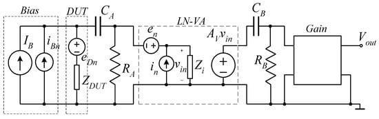
Figure 8.
Block diagram of basic set up for voltage noise measurements.
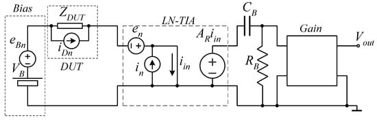
Figure 9.
Block diagram of basic set up for current noise measurements.
Assuming now, as it is often the case, that the noise introduced by the second stage is negligible, because of the large gain of the first stage, we can interpret the power spectral density (PSD) of the noise at the output of the amplifier as due to an equivalent input voltage PSD SVin given by:
where SIBN is the PSD of the noise source iBn, SVDN is the PSD of the noise source eDn (i.e., the noise source generated by the DUT), and SVN is the PSD of the equivalent input noise source of the LN-VA.
Clearly, SVin can be assumed to represent SVDN only if SVN and the effect of SIBN are negligible. As far as SIBN is concerned, a few designs for the realization of low noise current sources have been proposed [99,100,101,102]. Depending on the current range to be sourced, the designs may vary considerably and, actually, there is no single approach than can be considered sufficiently general to be regarded as a reference design for the implementation of high sensitivity, low frequency voltage noise measurement systems. In most cases, if fine tuning of the current is not required, the current source in Figure 8 is obtained starting from a battery with a resistance in series that is much larger than the DUT impedance as in Figure 10.
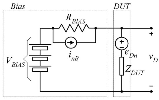
Figure 10.
Block diagram for the calculation of the contribution to the voltage noise across the DUT as due to the bias network.
If the current supplied by the batteries (VBIAS) is a small fraction of their maximum rated value, they behave as very low noise voltage sources, and if the resistance in series (RBIAS) is a high quality metallic film resistance, its contribution can be reduced to its thermal noise. If, for the sake of simplicity, we assume the DUT to behave as a resistance with value RD << RBIAS, from Figure 10 we can calculate that the contribution to the voltage noise across the DUT as due to the bias network is:
where SVTH(RD) is the thermal noise of the DUT. Equation (10) is particularly interesting when we observe that in order to detect low frequency noise generated by the DUT, its level must necessarily be above the thermal noise of the DUT.
Therefore, since the noise contribution of the bias network is always below the thermal noise of the DUT (RD << RBIAS), in the bias configuration in Figure 10 the noise introduced by the bias network is always negligible. Note that the condition RD << RBIAS is also required since, in Figure 10, the contribution of the noise coming from the DUT is attenuated because of the presence of a finite RBIAS. However, as long as RBIAS >> RD, the attenuation is small and can be usually neglected.
As we have noted above, in order to obtain very low level of BN at very low frequencies (f < 1 Hz) we need to resort to discrete devices for the front end of the LN-VA. In order to understand the advantage that can be obtained in terms of BN when resorting to discrete JFETs, it is sufficient to observe that if we resorted to the conventional OA based voltage amplifier topology for the realization of the LN-VA, the equivalent input voltage noise source en in Figure 8 could be made to essentially coincide with the equivalent input voltage noise of the OA. The JFET input operational amplifiers with the lowest level of equivalent input voltage noise that we have been able to find are the ones belonging to the OPAx140 series by Texas Instruments [103]. Their equivalent input voltage noise is about 50 nV/√Hz at 100 mHz, less than 16 nV√Hz at 1 Hz, and about 5 nV√Hz for f > 1 kHz. If, on the other hand, we design the LN-VA using the very large area IF3601 by InterFet [104], the equivalent input voltage noise can be as low as 5.6 nV/√Hz at 100 mHz and 1.4 nV/√Hz [95], with a gain, in terms of BN PSD reduction of 80 and 13 at 100 mHz and 1 Hz, respectively. While obtaining the ultimate noise performances in discrete JFET based amplifiers may require resorting to relatively complex circuitry [94,95], optimized design aimed at simplifying implementation while maintaining excellent noise performances have been proposed. For instance, Figure 11 reports the complete schematic of the amplifier proposed in [96] that, with a very limited component count, allows to obtain an equivalent input noise of about 14, 1.4, and 0.8 nV/√Hz at 100 mH, 1 Hz, and for f > 1 kHz, respectively.
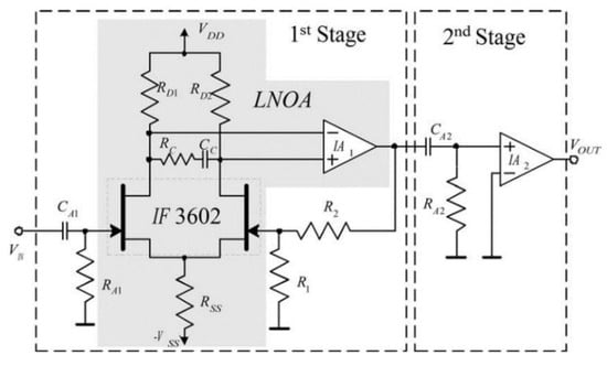
Figure 11.
Complete schematic of the Low Noise Voltage Amplifier (LN-VA) proposed in [96].
A fully differential input low noise amplifier can be derived from the circuit in Figure 11 for noise measurement across a DUT with none of the two terminals grounded [105].
Voltage noise measurements are typically employed for low to moderate impedances for the DUTs (from a few Ω up to a few tens of kΩ), where all the conditions that allow to simplify the measurement set up discussed above can be met. For much higher impedances, current noise measurements are usually more easily implemented. In principle, one could assume that current noise measurements present issues that are dual with respect to the case of voltage noise measurements, but in the case of low frequency noise measurements this is seldom the case. As we have discussed above, in the case of voltage noise measurements, AC coupling down to the tens of mHz range for removing the DC component can be obtained with simple RC networks (RACA in Figure 9) with reasonable values (MΩ for the resistances and tens of μF for the capacitances) with the capacitors only marginally deviating from ideality. In the case of current noise measurement, we would require an input AC coupling network capable of separating the DC bias current from the current fluctuations down to the mHz range. This could be done, in principle, by employing the circuit configuration in Figure 12 in which the LARA network would operate dually with respect to the RACA network in Figure 11. However, even assuming a resistance RL in the order of 1 kΩ (in the case of current measurements RL must be much lower with respect to the impedance of the DUT for its attenuation effect to be negligible) the value of LA that would be required to obtain a low frequency corner below 100 mHz would be larger than 1 kH, that is, to say the least, completely outside the range of values that can be realized, at least with high quality and for signal applications.
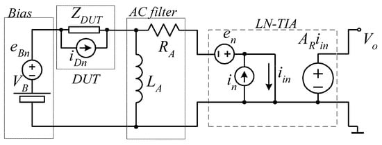
Figure 12.
Ideal circuit for separating the current fluctuations entering the Low Noise Transimpedance Amplifier (LN-TIA) from the DC bias current (ideally flowing through the inductance LA).
This means, as it is shown in Figure 9, that the first stage (the transimpedance amplifier) is always coupled in DC, and this translates in an important constraint in the performances that can be obtained by a low noise transimpedance amplifier as we shall presently discuss. To this purpose, rather than dealing with the general circuit configuration in Figure 9 it is convenient to refer to the actual circuit configurations employed for the realization of Low Noise Transimpedance Amplifier (LN-TIA). In almost any instance of low frequency noise measurements, the basic circuit configuration that is employed is shown in Figure 12.
The operational amplifier in Figure 13 is a JFET or MOSFET input operational amplifier, so that the current noise sources that are present at its inputs can be typically neglected with respect to other sources of noise [106]. The operational amplifier equivalent input voltage noise source eVn is shown explicitly in the figure as its effect can be relevant especially at higher frequencies and in the case of DUTs with large capacitive components, as it will be presently discussed. With the equivalent circuit in Figure 10 in mind, in the assumption of virtual short circuit between the inverting and non-inverting inputs of the operational amplifier, the transresistance gain AR can be calculated to be -RR while for the equivalent input voltage and current noise sources en and in we have:
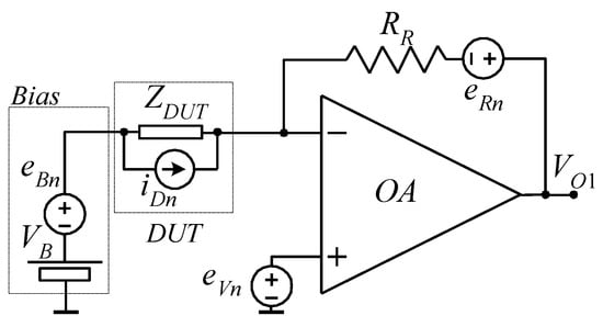
Figure 13.
Reference circuit for current noise measurements.
As it is apparent from Equation (11), the equivalent sources in and en are correlated since eVn contributes to both sources. The noise introduced by the feedback resistance (RR) is due to its thermal noise and its power spectra density SVR is given by:
For resistances RR in excess of 1 MΩ, the thermal noise of the resistance is much larger than 1 × 10⁻¹⁴ V2/Hz (or 100 nV/√Hz) so that, unless we need to work at very low frequencies (f << 1Hz), the contribution of eVn to the equivalent input noise in can be neglected (the PSD of eVn for the TLC 2201 MOSFET input OA is in the order 3.6 × 10⁻¹⁵ V2/Hz at 1 Hz and 43.6 × 10⁻¹⁶ V2/Hz at 10 Hz). In this assumption we obtain, for the PSD SIN of the equivalent input noise source in:
Equation (13) is particularly interesting since it shows that in order to reduce the equivalent input noise of a LN-TIA realized as in Figure 13 the feedback resistance must be made as large as possible. Unfortunately, since also the bias current flows through the feedback resistance, there is a limit at the maximum value of RR that can be used. If IB is DC bias current sourced by VB, the DC output voltage VODC1 at the output VO1 in Figure 13 is:
For the OA in Figure 13 to remain in linearity, VODC1 must remain within the power supply voltages, typically a few V. Therefore, in performing current noise measurements we are in a situation where we could, in principle, obtain an equivalent input current noise as low as desired, by increasing the feedback resistance. However, increasing RR reduces proportionally the maximum current that can flow through the DUT. The fact that the DC output voltage is proportional to the bias current flowing through the DUT has however one useful outcome: by measuring the DC voltage at the output VO1, we obtain the value of the DC current through the DUT for any given bias voltage VB. The AC filter CBRB in Figure 9 is used to remove the (large) DC component and to allow the amplification of the noise only up to a level compatible with the dynamic of the signal acquisition and elaboration system used for spectral estimation.
In order to evaluate the overall noise contribution to the output and to analyze to what extent the output noise in the circuit in Figure 13 can be regarded as essentially due to the DUT we must also take into account the effect of the noise introduced by the bias system (eBn) and the noise introduced by the equivalent input voltage noise eVn when regarded as responsible for the equivalent input voltage noise en. The voltage noise VOn at the output VO1 can be obtained as:
The PSD of VOn can be then obtained as (the noise sources in Equation (15) are uncorrelated):
By dividing Equation (16) by the transresistance gain squared (RR2) we can interpret the noise at the output as due to the PSD SIN of a current source at the input of a noiseless TIA with the same gain:
Cleary we can interpret SIN as due to the DUT (SID) as long as all other contributions can be neglected. In a situation in which a sufficiently large RR can be used for reducing the contribution of its thermal noise to a negligible level, the noise introduced by the equivalent input voltage noise of the amplifier and from the bias system may become relevant. If the impedance of the DUT is large or in the same order of the feedback resistance and the noise introduced by the bias system is comparable to that due to the equivalent input voltage noise of the amplifier, the argument leading to Equation (13) can be extended to Equation (17) and, at least at low frequencies, the contributions by SVV and SVB can be assumed negligible. However, if the DUT has a significant parallel capacitive component, that can also be the result of the parasitic capacitances in the cables connecting the DUT to the system, the impedance of the DUT decreases with frequency and the noise introduced by SVV (and possibly by SVB) can soon mask the noise coming from the DUT [107]. Note, moreover, that methods have been proposed that allow to reduce the noise introduced by the feedback resistance either by cross correlation approaches [108,109] or by exploiting configurations in which the feedback impedance is replaced by a capacitor that, intrinsically, does not introduce noise (noise however, is still introduced by the DC path required to close the DC feedback path from the output of the OA to the inverting input) [110,111,112]. In all these cases, the ultimate level of background noise is set by the equivalent input voltage noise source of the operational amplifier, assuming that the noise of the bias system can be made negligible.
As far as the bias system is concerned, in the configuration in Figure 13 it is the voltage source VB that supplies the DC current to the DUT. A different configuration can be used, however, in which the voltage source providing the voltage bias does only supply the extremely low current required to bias the non-inverting input of the OA. This circuit configuration is shown in Figure 14.
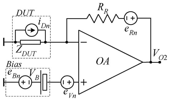
Figure 14.
Alternative circuit for current noise measurements.
Due to the virtual short between the inputs of the operational amplifier, the voltage bias across the DUT in Figure 14 is the same as in Figure 13 for the same value of VB. The voltage source VB must only supply the very low bias current at the input of the JFET (or MOSFET) input operational amplifier. Moreover, in this configuration the DUT has got one terminal connected to system ground. The price to be paid is the fact that in the circuit in Figure 14, the DC output voltage VODC2 is:
According to Equation (18), is larger than in Equation (14) for the same bias condition for the DUT. This results in a lower maximum bias current for remaining in linearity or, to maintain the same maximum bias current as in Figure 13, a lower value for RR and, hence, a higher level of background noise.
The circuit topologies and design guidelines summarized above can be used for the development of dedicated instrumentation tailored to the specific sensing application at hand. System integration, that is the ability to combine and optimize the electronics sections together with the mechanical structure (for support and for electromagnetic shielding) and dedicated control and data elaboration software can play a significant role in the realization of effective and user friendly noise measurement systems [70,71,113,114,115,116].
7. Conclusions
We highlighted the problems and limitations of classic gas and odors sensing and discussed, also illustrating its history, the fluctuation-enhanced sensing technique as a valid and powerful alternative. The main practical problems to be addressed when applying FES were also addressed and possible solutions were proposed. The body of literature on FES indicates that FES platforms have become mature enough to leave the fundamental investigation and prototype stage and join the R&D of commercial sensor systems. We believe that a major role will be played by the development of low noise electronics capable of achieving a sufficiently low level of background noise. Moreover, while excellent performance can be obtained by relatively simple measurement systems at fixed conditions (laboratory or indoor environment), the development of versatile and reliable electronic noses require substantial R&D phase. Major issues are the mode of operation, selection of materials, structures (including contact methods), sensitivity, selectivity, circuitry, computational power and energy dissipation, portability, and networking.
Author Contributions
Conceptualization, G.S., J.S. and L.B.K.; methodology, G.S., J.S. and L.B.K.; validation, G.S., J.S. and L.B.K.; formal analysis, G.S., J.S. and L.B.K.; investigation, G.S., J.S. and L.B.K.; data curation, G.S., J.S. and L.B.K.; writing—original draft preparation, G.S., J.S. and L.B.K.; writing—review and editing, G.S., J.S. and L.B.K.; visualization, G.S., J.S. and L.B.K.; supervision, G.S., J.S. and L.B.K.; project administration, G.S., J.S. and L.B.K. All authors have read and agreed to the published version of the manuscript.
Funding
This research received no external funding.
Conflicts of Interest
The authors declare no conflict of interest.
References
- Ghaffarpasand, O.; Beddows, D.C.S.; Ropkins, K.; Pope, F.D. Real-world assessment of vehicle air pollutant emissions subset by vehicle type, fuel and EURO class: New findings from the recent UK EDAR field campaigns, and implications for emissions restricted zones. Sci. Total Environ. 2020, 734, 139416. [Google Scholar] [CrossRef]
- Wang, Y.; Zhao, Y.; Zhang, L.; Zhang, J.; Liud, Y. Modified regional biogenic VOC emissions with actual ozone stress and integrated land cover information: A case study in Yangtze River Delta, China. Sci. Total Environ. 2020, 727, 138703. [Google Scholar] [CrossRef]
- Collier-Oxandale, A.; Wong, N.; Navarro, S.; Johnston, J.; Hannigan, M. Using gas-phase air quality sensors to disentangle potential sources in a Los Angeles neighborhood. Atmos. Environ. 2020, 233, 117519. [Google Scholar] [CrossRef]
- Aguilar, C.M.Z.; Valdes-Manzanilla, A.; Margulis, R.B.; Meraz, E.D.A. Comparison between simulated SO2 concentrations using satellite emission data and Pemex emission inventories in Tabasco, Mexico. Environ. Monit. Assess. 2020, 192, 310. [Google Scholar] [CrossRef] [PubMed]
- Idrees, Z.; Zheng, L. Low cost air pollution monitoring systems: A review of protocols and enabling technologies. J. Ind. Inf. Integr. 2020, 17, 100123. [Google Scholar] [CrossRef]
- Leifer, I.; Melton, C.; Chatfield, R.; Cui, X.; Fischer, M.L.; Fladeland, M.; Gore, W.; Hlavka, D.L.; Iraci, L.T.; Marrero, J.; et al. Air pollution inputs to the Mojave Desert by fusing surface mobile and airborne in situ and airborne and satellite remote sensing: A case study of interbasin transport with numerical model validation. Atmos. Environ. 2020, 224, 117184. [Google Scholar] [CrossRef]
- Ministry of Environmental Protection. Ministry of Environmental Protection of the People’s Republic of China. Technical Regulation on Ambient Air Quality Index 2012. Available online: https://web.archive.org/web/20130820070548/http://kjs.mep.gov.cn/hjbhbz/bzwb/dqhjbh/jcgfffbz/201203/W020120410332725219541.pdf (accessed on 21 August 2020).
- United States Environmental Protection Agency. Air quality Index (AQI)—A Guide to Air Quality and Your Health. Available online: https://www3.epa.gov/airnow/aqi_brochure_02_14.pdf (accessed on 21 August 2020).
- Snyder, E.G.; Watkins, T.H.; Solomon, P.A.; Thomas, E.D.; Williams, R.W.; Hagler, G.S.; Shelow, D.; Hindin, D.A.; Kilaru, V.J.; Preuss, P.W. The changing paradigm of air pollution monitoring. Environ. Sci. Technol. 2013, 47, 11369–11377. [Google Scholar] [CrossRef] [PubMed]
- White, R.M.; Paprotny, I.; Doering, F.; Cascio, W.E.; Solomon, P.A.; Gundel, L.A. Sensors for community-based atmospheric monitoring EM: Air and Waste Management Association’s. Mag. Environ. Manag. 2012, 5, 36–40. [Google Scholar]
- Murota, K.; Hirade, K. GMSK Modulation for Digital Mobile Radio Telephony. IEEE Trans. Commun. 2001, 29, 1044–1050. [Google Scholar] [CrossRef]
- Raul, I.; Gabriel, V.; Septimiu, M. GPRS Based Data Acquisition and Analysis System with Mobile Phone. Control Meas. 2012, 45, 1462–1470. [Google Scholar]
- Brown, S.K.; Sim, M.R.; Abramson, M.J.; Gray, C.N. Concentrations of Volatile Organic Compounds in Indoor Air—A Review. Indoor Air 1994, 4, 123. [Google Scholar] [CrossRef]
- World Health Organization. Indoor Air Pollutants: Exposure and Health Effects; EURO Reports and Studies NO. 78; WHO Regional Office for Europe: Copenhagen, Denmark, 1983. [Google Scholar]
- Horvath, E.P. Building-related illness and sick building syndrome: From the specific to the vague. Clevel. Clin. J. Med. 1997, 64, 3031. [Google Scholar] [CrossRef] [PubMed]
- Silva, L.M. Air Distribution in Rooms, (ROOMVENT 2000); Awbi, H.B., Ed.; Elsevier Science: London, UK, 2000; p. 13. [Google Scholar]
- Li, F.; Cai, H.; Xu, J.; Zhang, K.; Feng, Q.; Wang, H. Gas distribution mapping for indoor environments based on laser absorption spectroscopy: Development of an improved tomographic algorithm. Build. Environ. 2020, 172, 106724. [Google Scholar] [CrossRef]
- Taguchi, N. Gas Detecting Element and Method of Making it. US Patent No. 3,644,795, 22 February 1972. [Google Scholar]
- Eranna, G.; Joshi, B.C.; Runthala, D.P.; Gupta, R.P. Oxide Materials for Development of Integrated Gas Sensors—A Comprehensive Review. Crit. Rev. Solid State Mater. Sci. 2004, 29, 111. [Google Scholar] [CrossRef]
- Lin, Y.; Fan, Z. Compositing strategies to enhance the performance of chemiresistive CO2 gas sensors. Mater. Sci. Semicond. Process. 2020, 107, 104820. [Google Scholar] [CrossRef]
- Lin, H.M.; Hsu, C.H.; Yang, H.Y.; Lee, P.Y.; Yang, C.C. Nanocrystalline WO3-based H2S sensors. Sens. Actuators B 1994, 22, 63. [Google Scholar] [CrossRef]
- Hoel, A. Electrical Properties of Nanocrystalline WO3 for Gas Sensing Applications. Ph.D. Thesis, Acta Universitatis Upsaliensis, Uppsala, Sweden, 2004. [Google Scholar]
- Wang, X.; Yee, S.S.; Carey, W.P. Transition between Neck-Controlled and Grain-Boundary-Controlled Sensitivity of Metal-Oxide Gas Sensors. Sens. Actuators B 1995, 25, 454. [Google Scholar] [CrossRef]
- Reyes, L.F.; Hoel, A.; Saukko, S.; Heszler, P.; Lantto, V.; Granqvist, C.G. Gas sensor response of pure and activated WO3 nanoparticle films made by advanced reactive gas deposition. Sens. Actuators B 2006, 117, 128. [Google Scholar] [CrossRef]
- Malik, R.; Tomer, V.K.; Mishra, Y.K.; Lin, L. Functional gas sensing nanomaterials: A panoramic view. Appl. Phys. Rev. 2020, 7, 021301. [Google Scholar] [CrossRef]
- Panayotova, M.; Panayotov, V.; Oliinyk, T. Gallium and indium nanomaterials for environmental protection. In Proceedings of the International Conference on Sustainable Futures: Environmental, Technological, Social and Economic Matters (ICSF 2020), Kryvyi Rih, Ukraine, 20–22 May 2020; E3S Web Conference 2020. Volume 166. [Google Scholar] [CrossRef]
- Gardner, J.W.; Bartlet, P.N. Electronic Noses: Principles and Applications; Oxford University Press: Oxford, UK, 1999. [Google Scholar]
- Hines, E.L.; Llobet, E.; Gardner, J.W. Electronic noses: A review of signal processing techniques. IEE Proc. Circuits Devices Syst. 1999, 146, 297. [Google Scholar] [CrossRef]
- Hayasaka, T.; Lin, A.; Copa, V.C.; Lopez, L.P., Jr.; Loberternos, R.A.; Ballesteros, L.I.M.; Kubota, Y.; Liu, Y.; Salvador, A.A.; Lin, L. An electronic nose using a single graphene FET and machine learning for water, methanol, and ethanol. Microsyst. Nanoeng. 2020, 6, 50. [Google Scholar] [CrossRef]
- Ionescu, R.; Hoel, A.; Granqvist, C.G.; Llobet, E.; Heszler, P. Low-level detection of ethanol and H2S with temperature- modulated WO3 nanoparticle gas sensors. Sens. Actuators B 2005, 104, 132. [Google Scholar] [CrossRef]
- Faleh, R.; Bedoui, S.; Kachouri, A. Review on Smart Electronic Nose coupled with Artificial Intelligence for Air Quality Monitoring. Adv. Sci. Technol. Eng. Syst. J. 2020, 5, 739–747. [Google Scholar] [CrossRef]
- Kish, L.B.; Schmera, G.; Kwan, C.; Smulko, J.; Heszler, P.; Granqvist, C.G. Fluctuation-enhanced sensing. Keynote Invited Talk. In Proceedings of the Conference on Noise in Materials, Devices and Circuits at SPIE’s Fourth International Symposium on Fluctuations and Noise (FaN’07), Florence, Italy, 20–24 May 2007. [Google Scholar]
- White, D.R.; Galleano, R.; Actis, A.; Brixy, H.; de Groot, M.; Dubbeldam, J.; Reesink, A.L.; Edler, F.; Sakurai, H.; Shepard, R.L.; et al. The status of Johnson noise thermometry. Metrologia 1996, 33, 325–335. [Google Scholar] [CrossRef]
- Ayhan, B.; Kwan, C.; Zhou, J.; Kish, L.B.; Benkstein, K.D.; Rogers, P.H.; Semancik, S. Fluctuation enhanced sensing (FES) with a nanostructured, semiconducting metal oxide film for gas detection and classification. Sens. Actuators B Chem. 2013, 188, 651–660. [Google Scholar] [CrossRef]
- Makra, P.; Topalian, Z.; Granqvist, C.G.; Kish, L.B.; Kwan, C. Accuracy versus speed in fluctuation-enhanced sensing. Fluct. Noise Lett. 2012, 11, 1250010. [Google Scholar] [CrossRef]
- Gingl, Z.; Kish, L.B.; Ayhan, B.; Kwan, C.; Granqvist, C.-G. Fluctuation-Enhanced Sensing with Zero-Crossing Analysis for High-Speed and Low-Power Applications. IEEE Sens. J. 2010, 10, 492–497. [Google Scholar] [CrossRef]
- Chang, H.C.; Kish, L.B.; King, M.D.; Kwan, C. Fluctuation-Enhanced Sensing of Bacterium Odors. Sens. Actuators B 2009, 142, 429–434. [Google Scholar] [CrossRef][Green Version]
- Kwan, C.; Schmera, G.; Smulko, J.; Kish, L.B.; Heszler, P.; Granqvist, C.G. Advanced agent identification at fluctuation-enhanced sensing. IEEE Sens. J. 2008, 8, 706–713. [Google Scholar] [CrossRef]
- Aroutiounian, M.; Mkhitaryan, Z.; Adamian, A.; Granqvist, C.-G.; Kish, L.B. Fluctuation-enhanced gas sensing. Procedia Chem. 2009, 1, 216–219. [Google Scholar] [CrossRef]
- Kish, L.B.; Schmera, G.; King, M.D.; Cheng, M.; Young, R.; Granqvist, C.G. Fluctuation-Enhanced Chemical/Biological Sensing and Prompt Identification of Bacteria by Sensing of Phage Triggered Ion Cascade (SEPTIC). Intern. J. High. Speed Electron. Syst. 2008, 18, 11–18. [Google Scholar] [CrossRef]
- Bruschi, P.; Cacialli, F.; Nannini, A.; Neri, B. Gas and vapour effects on the resistance fluctuation spectra of conducting polymer thin-film resistors. Sens. Actuators B 1994, 19, 421. [Google Scholar] [CrossRef]
- Bruschi, P.; Nannini, A.; Neri, B. Vapour and gas sensing by noise measurements on polymeric balanced bridge microstructures. Sens. Actuators B 1995, 25, 429. [Google Scholar] [CrossRef]
- Gottwald, P.; Kincses, Z.; Szentpali, B. Unsolved Problems of Noise (UPoN’96); Doering, C.R., Kiss, L.B., Shlesinger, M.F., Eds.; World Scientific: Singapore, 1997; p. 122. [Google Scholar]
- Kiss, L.B.; Granqvist, C.G.; Söderlund, J. Detection of Chemicals Based on Resistance Fluctuation Spectroscopy. Swedish Patent, Ser 9803019-0, 17 July 2000. [Google Scholar]
- Kiss, L.B.; Vajtai, R.; Granqvist, C.G. Unsolved Problems of Noise and Fluctuations. In Proceedings of the 2nd International Conference on Unsolved Problems of Noise (UPoN’99), Adelaide, Australia, 11–15 July 1999; American Institute of Physics: Melville, NY, USA, 2000; p. 463. [Google Scholar]
- Kish, L.B.; Vajtai, R.; Granqvist, C.-G. Extracting information from noise spectra of chemical sensors:single sensor electronic noses and tongues. Sens. Actuators B 2000, 71, 55. [Google Scholar] [CrossRef]
- Solis, J.L.; Kish, L.B.; Vajtai, R.; Granqvist, C.G.; Olsson, J.; Schnurer, J.; Lantto, V. Identifying natural and artificial odors through noise analysis with a sampling-and-hold electronic nose. Sens. Actuators B 2001, 77, 312. [Google Scholar] [CrossRef]
- Smulko, J.; Granqvist, C.G.; Kish, L.B. On the statistical analysis of noise in chemical sensors and its application for sensing. Fluct. Noise Lett. 2001, 1, L14722. [Google Scholar] [CrossRef]
- Smulko, J.; Ederth, J.; Kish, L.B.; Heszler, P.; Granqvist, C.G. Higher-order spectra in nanoparticle gas sensors. Fluct. Noise Lett. 2004, 4, L597. [Google Scholar] [CrossRef]
- Smulko, J.M.; Kish, L.B. Higher-Order Statistics for Fluctuation-Enhanced Gas-Sensing. Sens. Mater. 2004, 16, 291–299. [Google Scholar]
- Smulko, J.M.; Ederth, J.; Li, Y.; Kish, L.B.; Kennedy, M.K.; Kruis, F.E. Gas sensing by thermoelectric voltage fluctuations in SnO2 nanoparticle films. Sens. Actuators B 2005, 106, 708. [Google Scholar]
- Hoel, A.; Ederth, J.; Kopniczky, J.; Heszler, P.; Kish, L.B.; Olsson, E.; Granqvist, C.G. Conduction invasion noise in nanoparticle WO3/Au thin-film devices for gas sensing application. Smart Mater. Struct. 2002, 11, 640–644. [Google Scholar] [CrossRef]
- Schmera, G.; Kish, L.B. Fluctuation Enhanced Chemical Sensing by Surface Acoustic Wave Devices. Fluct. Noise Lett. 2002, 2, L117–L123. [Google Scholar] [CrossRef]
- Schmera, G.; Kish, L.B. Surface diffusion enhanced chemical sensing by surface acoustic waves. Sens. Actuators B 2003, 93, 159–163. [Google Scholar] [CrossRef]
- Solis, J.L.; Seeton, G.; Li, Y.; Kish, L.B. Fluctuation-Enhanced Sensing with Commercial Gas Sensors. Sens. Transducers Mag. 2003, 38, 59–66. [Google Scholar]
- Kish, L.B.; Li, Y.; Solis, J.L.; Marlow, W.H.; Vajtai, R.; Granqvist, C.G.; Lantto, V.; Smulko, J.M.; Schmera, G. Detecting harmful gases using fluctuation-enhanced sensing with Taguchi sensors. IEEE Sens. J. 2005, 5, 671. [Google Scholar] [CrossRef]
- Solis, J.L.; Seeton, G.E.; Li, Y.; Kish, L.B. Fluctuation-Enhanced Multiple-Gas Sensing. IEEE Sens. J. 2005, 5, 1338–1345. [Google Scholar] [CrossRef]
- Ederth, J.; Smulko, J.M.; Kish, L.B.; Heszler, P.; Granqvist, C.G. Comparison of classical and fluctuation-enhanced gas sensing with PdxWO3 nanoparticle films. Sens. Actuators B 2006, 113, 310–315. [Google Scholar] [CrossRef]
- Gomri, S.; Seguin, J.L.; Aguir, K. Modelling on oxygen–chemisorption—Induced noise in metallic oxide gas sensors. Sens. Actuators B 2005, 107, 722. [Google Scholar] [CrossRef]
- Gomri, S.; Seguin, J.L.; Guerin, J.; Aguir, K. Adsorption-desorption noise in gas sensors: Modelling using Langmuir and Wolkenstein models for adsorption. Sens. Actuators B 2006, 114, 451. [Google Scholar] [CrossRef]
- Gomri, S.; Seguin, J.; Contaret, T.; Fiorido, T.; Aguir, K. A Noise Spectroscopy-Based Selective Gas Sensing with MOX Gas Sensors. Fluct. Noise Lett. 2018, 17, 1850016. [Google Scholar] [CrossRef]
- Huang, G.H.; Deng, S.P. The conception, structure and techniques on the artificial taste system. Prog. Chem. 2006, 18, 494. [Google Scholar]
- Molnár, D.; Heszler, P.; Mingesz, R.; Gingl, Z.; Kukovecz, Á.; Kónya, Z.; Haspel, H.; Mohl, M.; Sápi, A.; Kiricsi, I.; et al. Increasing chemical selectivity of carbon nanotube-based sensors by fluctuation-enhanced sensing. Fluct. Noise Lett. 2010, 09, 277–287. [Google Scholar] [CrossRef]
- Kukovecz, A.; Heszler, P.; Kordás, K.; Roth, S.; Kónya, Z.; Haspel, H.; Ionescu, R.; Sápi, A.; Maklin, J.; Mohl, M.; et al. Improving the performance of functionalized carbon nanotube thin film sensors by fluctuation enhanced sensing. In Proceedings of the SPIE—The International Society for Optical Engineering, Carbon Nanotubes and Associated Devices, San Diego, CA, USA, 10–12 August 2008; Volume 7037. [Google Scholar] [CrossRef]
- Heszler, P.; Gingl, Z.; Mingesz, R.; Csengeri, A.; Haspel, H.; Kukovecz, A.; Kónya, Z.; Kiricsi, I.; Ionescu, R.; Mäklin, J.; et al. Drift effect of fluctuation enhanced gas sensing on carbon nanotube sensors. Phys. Status Solidi (B) Basic Res. 2008, 245, 2343–2346, Special Issue: Electronic Properties of Novel Materials: “Molecular nanostructures”. [Google Scholar] [CrossRef]
- Kukovecz, Á.; Molnár, D.; Kordás, K.; Gingl, Z.; Moilanen, H.; Mingesz, R.; Kónya, Z.; Mäklin, J.; Halonen, N.; Tóth, G.; et al. Carbon nanotube based sensors and fluctuation enhanced sensing. Phys. Status Solidi (C) Curr. Top. Solid State Phys. 2010, 7, 1217–1221. [Google Scholar] [CrossRef]
- Macucci, M.; Marconcini, P. Theoretical Comparison between the Flicker Noise Behavior of Graphene and of Ordinary Semiconductors. Hindawi J. Sens. 2020, 2020, 2850268. [Google Scholar] [CrossRef]
- Kuberský, P.; Sedlák, P.; Hamáček, A.; Nešpůrek, S.; Kuparowitz, T.; Šikula, J.; Majzner, J.; Sedlaková, V.; Grmela, L.; Syrový, T. Quantitative fluctuation-enhanced sensing in amperometric NO2 sensors. Chem. Phys. 2015, 456, 111–117. [Google Scholar] [CrossRef]
- Sedlak, P.; Kubersky, P.; Skarvada, P.; Hamacek, A.; Sedlakova, V.; Majzner, J.; Nespurek, S.; Sikula, J. Current fluctuation measurements of amperometric gas sensors constructed with three different technology procedures. Metrol. Meas. Syst. 2016, 23, 531–543. [Google Scholar] [CrossRef]
- Mingesz, R.; Gingl, Z.; Kukovecz, Á.; Kónya, Z.; Kordás, K.; Moilanen, H. Compact USB measurement and analysis system for real-time fluctuation enhanced sensing. In Proceedings of the 21st International Conference on Noise and Fluctuations, Toronto, ON, Canada, 12–16 June 2011. [Google Scholar]
- Gingl, Z.; Mingesz, R.; Vadai, G.; Balogh, K.S.; Erdélyi, Á. Fluctuation enhanced gas detector for wireless sensor networks. In Proceedings of the 22nd International Conference on Noise and Fluctuations (ICNF), Montpellier, France, 24–28 June 2013. [Google Scholar]
- Mingesz, R.; Makan, D.G.; Balogh, B.; Vadai, G.; Gingl, Z. IoT framework for Fluctuation Enhanced Sensing. In Proceedings of the 24st International Conference on Noise and Fluctuations (ICNF), Vilnius, Lithuania, 20–23 June 2017. [Google Scholar] [CrossRef]
- Kish, L.B.; Smulko, J.; Heszler, P.; Granqvist, C.G. On the sensitivity, selectivity, sensory information, and optimal size of resistive chemical sensors. Invited paper. Nanotechnol. Percept. 2007, 3, 43–52. [Google Scholar] [CrossRef]
- Kwan, C.; Ayhan, B.; Chen, G.; Chang, C.; Wang, J.; Ji, B. A Novel Approach for Spectral Unmixing, Classification, and Concentration Estimation of Chemical and Biological Agents. IEEE Trans. Geosci. Remote Sens. 2006, 44, 409–419. [Google Scholar] [CrossRef]
- Saletti, R. A comparison between two methods to generate 1/f γ noise. Proc. IEEE 1996, 74, 1595–1596. [Google Scholar] [CrossRef]
- Ciofi, C.; de Marines, M.; Neri, B. Ultralow-noise PC-based measurement system for the characterization of the metallization of integrated circuits. IEEE Trans. Instrum. Measur. 1997, 46, 789–793. [Google Scholar] [CrossRef]
- E4727A Advanced Low-Frequency Noise Analyzer. Available online: https://www.keysight.com/en/pd-2389560-pn-E4727A/advanced-low-frequency-noise-analyzer?nid=-32901.1082931&cc=US&lc=eng (accessed on 19 June 2020).
- Beyne, S.; Croes, K.; De Wolf, I.; Tőkey, Z. 1/f noise measurements for faster evaluation of electromigration in advanced microelectronic interconnections. J. Appl. Phys. 2016, 119, 184302. [Google Scholar] [CrossRef]
- Fleetwood, D.M.; Beyne, S.; Jiang, R.; Zhao, S.E.; Wang, P.; Bonaldo, S.; McCurdy, M.W.; Tőkei, Z.; DeWolf, I.; Croes, K.; et al. Low-frequency noise and defects in copper and ruthenium resistors. Appl. Phys. Lett. 2019, 114, 203501. [Google Scholar] [CrossRef]
- Ferrari, G.; Carminati, M.; Gervasoni, G.; Sampietro, M.; Prati, E.; Pennetta, C.; Lezzi, F.; Pisignano, D. High sensitivity noise measurements: Circuits, techniques and applications. In Proceedings of the 2015 International Conference on Noise and Fluctuations (ICNF), Xi’an, China, 2–6 June 2015. [Google Scholar]
- Chen, G.; Paronyan, T.M.; Pigos, E.M.; Harutyunyan, A.R. Enhanced gas sensing in pristine carbon nanotubes under continuous ultraviolet light illumination. Sci. Rep. 2012, 2, 343. [Google Scholar] [CrossRef] [PubMed]
- Comini, E.; Faglia, G.; Sberveglieri, G. UV light activation of tin oxide thin films for NO2 sensing at low temperatures. Sens. Actuators B Chem. 2001, 78, 73–77. [Google Scholar] [CrossRef]
- Prades, J.D.; Jiménez-Díaz, R.; Hernandez-Ramirez, F.; Barth, S.; Cirera, A.; Romano-Rodriguez, A.; Mathurcd, S.; Moranteae, J.R. Equivalence between thermal and room temperature UV light-modulated responses of gas sensors based on individual SnO2 nanowires. Sens. Actuators B Chem. 2009, 140, 337–341. [Google Scholar] [CrossRef]
- Gong, J.; Li, Y.; Chai, X.; Hu, Z.; Deng, Y. UV-light-activated ZnO fibers for organic gas sensing at room temperature. J. Phys. Chem. C 2009, 114, 1293–1298. [Google Scholar] [CrossRef]
- Trawka, M.; Smulko, J.; Hasse, L.; Granqvist, C.G.; Annanouch, F.E.; Ionescu, R. Fluctuation enhanced gas sensing with WO3-based nanoparticle gas sensors modulated by UV light at selected wavelengths. Sens. Actuators B Chem. 2016, 234, 453–461. [Google Scholar] [CrossRef]
- Trawka, M.P.; Smulko, J.M.; Hasse, L.Z.; Granqvist, C.G.; Ionescu, R.; Eduard, L.; Annanouch, F.E.; Kish, L.B. UV-light-induced fluctuation enhanced sensing by WO 3-based gas sensors. IEEE Sens. J. 2016, 16, 5152–5159. [Google Scholar] [CrossRef]
- Rumyantsev, S.; Liu, G.; Shur, M.S.; Potyrailo, R.A.; Balandin, A.A. Selective gas sensing with a single pristine graphene transistor. Nano Lett. 2012, 12, 2294–2298. [Google Scholar] [CrossRef]
- Topalian, Z.; Smulko, J.M.; Niklasson, G.A.; Granqvist, C.G. Resistance noise in TiO2-based thin film gas sensors under ultraviolet irradiation. J. Phys. Conf. Ser. 2007, 76, 012056. [Google Scholar] [CrossRef]
- Samnakay, R.; Jiang, C.; Rumyantsev, S.L.; Shur, M.S.; Balandin, A.A. Selective chemical vapor sensing with few-layer MoS2 thin-film transistors: Comparison with graphene devices. Appl. Phys. Lett. 2015, 106, 023115. [Google Scholar] [CrossRef]
- Rumyantsev, S.; Liu, G.; Potyrailo, R.A.; Balandin, A.A.; Shur, M.S. Selective sensing of individual gases using graphene devices. IEEE Sens. J. 2013, 13, 2818–2822. [Google Scholar] [CrossRef]
- Kish, L.B.; Granqvist, C.G.; Vajtai, R. Sampling-and-Hold Chemical Sensing by Noise Measurements for Electronic Nose Applications. Swedish Patent SE 9904209-5, 2 July 2001. Available online: http://was.prv.se/spd/pdf/RdizounvzhfWS3oljenFlQ/SE515249.C2.pdf (accessed on 19 June 2020).
- Chang, H.C.; Kish, L.B.; King, M.D.; Kwan, C. Binary Fingerprints at Fluctuation-Enhanced Sensing. Sensors 2010, 10, 361. [Google Scholar] [CrossRef] [PubMed]
- Kish, L.B.; Chang, H.C.; King, M.D.; Kwan, C.; Jensen, J.O.; Schmera, G.; Smulko, J.; Gingl, Z.; Granqvist, C.G. Fluctuation-Enhanced Sensing for Biological Agent Detection and Identification. IEEE Nanotechnol. 2011, 10, 1238–1242. [Google Scholar] [CrossRef]
- Neri, B.; Pellegrini, B.; Saletti, R. Ultra low-noise preamplifier for low-frequency noise measurements in electron devices. IEEE Trans. Instrum. Meas. 1991, 40, 2–6. [Google Scholar] [CrossRef]
- Levinzon, F.A. Ultra-low-noise high-input impedance amplifier for low-frequency measurement applications. IEEE Trans. Circuits Syst. I 2008, 55, 1815–1822. [Google Scholar] [CrossRef]
- Cannatà, G.; Scandurra, G.; Ciofi, C. An ultra low noise preamplifier for low frequency noise measurements. Rev. Sci. Instr. 2009, 80, 114702. [Google Scholar] [CrossRef]
- Serrano-Finetti, E.; Pallas-Areny, R. Noise reduction in AC-coupled amplifiers. IEEE Trans. Instrum. Meas. 2014, 63, 1834–1841. [Google Scholar] [CrossRef]
- Scandurra, G.; Cannatà, G.; Giusi, G.; Ciofi, C. A new approach to DC removal in high gain, low noise voltage amplifiers. In Proceedings of the 24st International Conference on Noise and Fluctuations (ICNF), Vilnius, Lithuania, 20–23 June 2017. [Google Scholar]
- Ciofi, C.; Giannetti, R.; Dattilo, V.; Neri, B. Ultra low noise current sources. IEEE Trans. Instrum. Meas. 1998, 47, 78–81. [Google Scholar] [CrossRef][Green Version]
- Talukdar, D.; Chakraborty, R.K.; Bose, S.; Bardhan, K.K. Low noise costant current source for bias dependent noise measurements. Rev. Sci. Instr. 2011, 82, 013906. [Google Scholar] [CrossRef]
- Scandurra, G.; Cannatà, G.; Giusi, G.; Ciofi, C. Programmable, very low noise current source. Rev. Sci. Instr. 2014, 85, 125109. [Google Scholar] [CrossRef] [PubMed]
- Scandurra, G.; Giusi, G.; Ciofi, C. A programmable bias current compensation approach in current noise measurement applications. In Proceedings of the IEEE International Instrumentation and Measurement Technology Conference (I2MTC), Auckland, New Zealand, 20–23 May 2019. [Google Scholar]
- Texas Instruments OPAx140 Datasheet. Available online: http://www.ti.com/lit/ds/symlink/opa140.pdf (accessed on 19 June 2020).
- IF3601 Datasheet. Available online: https://www.mouser.it/datasheet/2/676/jfet-if3601-interfet.r00-1649101.pdf (accessed on 19 June 2020).
- Scandurra, G.; Cannatà, G.; Ciofi, C. Differential ultra low noise amplifier for low frequency noise measurements. AIP Adv. 2011, 1, 022144. [Google Scholar] [CrossRef]
- Giusi, G.; Cannatà, G.; Scandurra, G.; Ciofi, C. Ultra-low-noise large-bandwidth transimpedance amplifier. Wiley Int. J. Circ. Theor. Appl. 2015, 43, 1455–1473. [Google Scholar] [CrossRef]
- Carminati, M.; Ferrari, G.; Sampietro, M.; Ivanov, A.P.; Albrecht, T. Low-noise dual-channel current amplifier for DNA sensing with solid-state nanopores. In Proceedings of the 19th IEEE International Conference on Electronics, Circuits, and Systems (ICECS 2012), Seville, Spain, 9–12 December 2012. [Google Scholar]
- Ciofi, C.; Scandurra, G.; Merlino, R.; Cannatà, G.; Giusi, G. A new correlation method for high sensitivity current noise measurement. Rev. Sci. Instrum. 2007, 78, 114702. [Google Scholar] [CrossRef]
- Scandurra, G.; Giusi, G.; Ciofi, C. Multichannel Amplifier Topologies for High-Sensitivity and Reduced Measurement Time in Voltage Noise Measurements. IEEE Trans. Instrum. Meas. 2013, 62, 1145–1153. [Google Scholar] [CrossRef]
- Ciofi, C.; Crupi, F.; Pace, C.; Scandurra, G. Improved trade-off between noise and bandwidth in op-amp based transimpedance amplifier. In Proceedings of the IEEE Instrumentation and Measurement Technology Conference, Como, Italy, 18–20 May 2004; Volume 3, pp. 1990–1993. [Google Scholar]
- Ciofi, C.; Crupi, F.; Pace, C.; Scandurra, G.; Patanè, M. A new circuit topology for the realization of very low-noise wide-bandwidth transimpedance amplifier. IEEE Trans. Instrum. Meas. 2007, 56, 1626–1631. [Google Scholar] [CrossRef]
- Ferrari, G.; Sampietro, M. Wide Bandwidth transimpedance amplifier for extremely high sensitivity continuous measurements. Rev. Scient. Instr. 2007, 78, 094703. [Google Scholar] [CrossRef]
- Ciofi, C.; Crupi, F.; Pace, C.; Scandurra, G. Micro-prober for wafer-level low-noise measurements in MOS devices. IEEE Trans. Instrum. Meas. 2003, 52, 1533–1536. [Google Scholar] [CrossRef]
- Giusi, G.; Giordano, O.; Scandurra, G.; Ciofi, C.; Rapisarda, M.; Calvi, S. Automatic measurement system for the DC and low-f noise characterization on FETs at wafer level. In Proceedings of the IEEE Instrumentation and Measurement Technology Conference, I2MTC, Pisa, Italy, 11–14 May 2015. [Google Scholar]
- Scandurra, G.; Beyne, S.; Giusi, G.; Ciofi, C. On the design of an automated system for the characterization of the electromigration performance of advanced interconnects by means of low-frequency noise measurements. Metrol. Meas. Syst. 2019, 26, 13–21. [Google Scholar]
- Trawka, M.; Smulko, J.; Chludziński, T. Portable measurement system for breath analysis by real-time fluctuation enhanced sensing method. In Proceedings of the 24st International Conference on Noise and Fluctuations (ICNF), Vilnius, Lithuania, 20–23 June 2017. [Google Scholar]


© 2020 by the authors. Licensee MDPI, Basel, Switzerland. This article is an open access article distributed under the terms and conditions of the Creative Commons Attribution (CC BY) license (http://creativecommons.org/licenses/by/4.0/).