Aerial Scene Classification through Fine-Tuning with Adaptive Learning Rates and Label Smoothing

Abstract

Remote Sensing (RS) image classification has recently attracted great attention for its application in different tasks, including environmental monitoring, battlefield surveillance, and geospatial object detection. The best practices for these tasks often involve transfer learning from pre-trained Convolutional Neural Networks (CNNs). A common approach in the literature is employing CNNs for feature extraction, and subsequently train classifiers exploiting such features. In this paper, we propose the adoption of transfer learning by fine-tuning pre-trained CNNs for end-to-end aerial image classification. Our approach performs feature extraction from the fine-tuned neural networks and remote sensing image classification with a Support Vector Machine (SVM) model with linear and Radial Basis Function (RBF) kernels. To tune the learning rate hyperparameter, we employ a linear decay learning rate scheduler as well as cyclical learning rates. Moreover, in order to mitigate the overfitting problem of pre-trained models, we apply label smoothing regularization. For the fine-tuning and feature extraction process, we adopt the Inception-v3 and Xception inception-based CNNs, as well the residual-based networks ResNet50 and DenseNet121. We present extensive experiments on two real-world remote sensing image datasets: AID and NWPU-RESISC45. The results show that the proposed method exhibits classification accuracy of up to 98%, outperforming other state-of-the-art methods.

1. Introduction

One task of computer vision is image classification and it has been thoroughly studied in the literature. There are many existing algorithms to solve this task. Remote sensing image classification is a more challenging problem due to the fact that objects are randomly rotated within a scene and the background texture is complex. The purpose of aerial scene classification techniques is to classify an image in one of the semantic classes, which are determined upon human interpretation. This problem has been of wide interest in resent research, due to its importance in a wide range of applications, including the surveillance of airports and aviation protection, flora monitoring in agriculture, and recognition of earth cover changes in environmental engineering [1].

RS image classification is possible thanks to the availability of RS images datasets that were collected from earth observation platforms, such as satellites, aerial systems, and unmanned aerial vehicles. The problem is complex and relies on the representation of salient image characteristics by means of high-level features. The latest techniques that include deep learning methods based on Convolutional Neural Networks (CNNs) have shown remarkable improvement in classification accuracy as compared to older ones based on handcrafted features [2,3]. The effectiveness of solutions based on CNNs lies in the possibility to perform knowledge transfer from pre-trained CNNs [4]. The knowledge transfer for image classification can be conducted in different ways, including feature extraction and fine-tuning [5,6].

There are numerous research studies that show that CNNs trained on one classification problem (such as ImageNet) can be successfully exploited to extract features from images in different tasks [7]. Excellent classification results were also achieved in aerial scene classification [8,9,10]. The first case of adoption of pre-trained CNN schemes for remote sensing image classification was performed by [8], where the pre-trained CNNs AlexNet and Overfeat [11] were employed for feature extraction, and the activations from the first fully connected layer of the CNN architectures were used as image representations. Excellent results with two remote sensing datasets are reported in [8], outperforming several handcrafted visual descriptors. The most popular approach for feature extraction using CNNs is to employ the extracted features from the upper convolutional layers, or the last fully connected layer that precedes the classification layers. However, when the target task of interest significantly differs from the original task, features extracted from lower convolutional layers appear to be more suitable [6].

The most widely used CNN models for aerial scene classification are CaffeNet, GoogleNet, and VGGNet [10,12,13,14,15]. These neural networks consist of approximately 30 layers and present a huge number of parameters. The study conducted in [16] evaluated deep features for the classification of traditional images, whether alone or combined with other features. Authors of [9] utilized extracted features from two pre-trained CNNs and, in that way, performed classification of high-resolution aerial scene images. They proposed features that were obtained by fusion of the activations from the mid-level layers and the last fully connected layers of the CNN schemes. Before feature fusion is performed, feature coding algorithms are applied to activations from convolutional layers. VGGNet is used for extracting features from different network layers, and then features are transformed by Discriminant Correlation Analysis (DCA) [13]. The transformed features are concatenated and, after that, a SVM classifier is applied for image classification [17]. The rationale of this process is to use convolution as an efficient way to extract a new compact and effective feature representation from raw data, simplifying the subsequent classification task. This capability of neural networks has also been fruitfully exploited in order to extract feature vector representations for predictive tasks also in the context of graph data [18,19] and time series data [20,21]. Feature fusion can also be found in other articles [22,23].

Two schemes are proposed in the literature. The former uses the original network for feature extraction from RGB images, while the mapped Local Binary Pattern (LBP) coded network is used for feature extraction from LBP feature maps. After this step, feature fusion is performed by the concatenation layer: features go through fully connected layers and they are classified at the end. The latter uses a saliency coded network instead of a mapped LBP coded network. The study [14] used Recurrent Neural Networks (RNNs) for remote sensing image classification. RNNs are employed to build the attention mechanism. In [12] is presented a new loss function, with enforcing metric learning to CNNs features. A metric learning loss was combined with a standard optimization loss (cross-entropy loss). This approach resulted in features that belong to images from the same image class to be very close, while features extracted from images from different classes to be very distant. The approach presented in [24] extracted features from different layers of pre-trained CNNs and concatenated them with prior dimensionality reduction through Principal Component Analysis (PCA). Logistic Regression Classifier (LRC) and SVMs were applied to the compound features. The classification accuracy of a pre-trained CNNs can be further improved through fine-tuning of the weights.

Fine-tuning is a transfer learning method that adjusts the parameters of a pre-trained CNN by resuming the training of the network with a new dataset, that possibly addresses a new task with a different number of classes than the initial output layer of the initial CNN architecture. Fine tuning trains the network with small initial learning rate and a reduced number of training epochs, compared to a complete training process from scratch. During this process, the cost function achieves a better minimum compared to a case with random weight initialization. Several articles [25,26] in the remote sensing community have also studied the advantages of fine-tuning pre-trained CNNs. Authors of [26] assessed a fully-trained CNN in comparison with a fine-tuned one, to discover utility in the context of aerial scene data. The approach presented in [25] employed the fine-tuning technique to classify hyperspectral images. Authors of [27] suggested to fine-tune the weights of the convolutional layers of the pre-trained CNN to extract better image features. The experimental results presented in [9,10] showed that fine tuning CNNs that are pre-trained on ImageNet gives good classification accuracy on aerial scene datasets.

In order to assess different techniques that exploit deep neural networks, authors of [28] evaluated the best scheme and training method, both for supervised and unsupervised networks. The study [29] tried to determine the optimal way to train neural networks, including greedy layer-wise and unsupervised training.

In this paper, we evaluate four different CNN architectures to solve the problem of high-resolution aerial scene classification. We adopt CNNs that are pre-trained on the ImageNet dataset with the purpose of determining their effectiveness in remote sensing image classification tasks. First, we explore the fine-tuning of the weights on the aerial image dataset. In the process of fine-tuning, we remove the final layers of each of the pre-trained networks after the average pooling layer (so called “network surgery”) and construct a new network head. The new network head consists of: a fully connected layer, dropout, and a softmax layer. Network training is performed on the modified deep neural network. Subsequently, we exploit fine-tuned CNNs for feature extraction and utilize the extracted features for the training of SVM classifiers, which have been successfully applied in other image classification and transfer learning problems [20,24,30]. In this paper, SVMs are implemented in two versions: with linear kernel and with Radial Basis Function (RBF) kernel. We use a linear decay learning rate schedule and cyclical learning rates and evaluate their suitability for fine-tuning of pre-trained CNNs for remote sensing image classification. Moreover, we apply label smoothing [31] as a regularization technique and assess its impact on the classification accuracy compared with state-of-the-art methods. Figure 1 shows a flowchart of the proposed method.

The main contributions of this paper are (1) evaluation of modern CNNs models on two remote sensing image datasets, (2) analysis of the impact of linear learning rate decay schedule and cyclical learning rates from the aspect of classification accuracy, (3) evaluation of label smoothing on model generalization compared to state-of-the-art techniques, and (4) assessment of the transferability of the features obtained from fine-tuned CNNs and their classification with linear and RBF SVMs classifiers. To the best of our knowledge, the combination of adaptive learning rate and label smoothing was never studied before in the context of aerial scene classification.

The remainder of this article is organized, as follows. In Section 2, the methodologies used for fine-tuning of CNNs are presented, and it is described how they were empirically evaluated. The experimental results obtained from the examined remote sensing image classification method are presented in Section 3. Discussion of our method results is given in Section 4. A summary of the results and conclusion of the paper, as well as directions for future research are presented in Section 5.

2. Methods

2.1. Convolutional Neural Networks (Cnns)

CNNs are suitable for many image-related problems, like image segmentation, classification, and object detection. CNN models are structures built from various layers concatenated one on top of the other. Layers consist of neurons that can learn through different optimization algorithms. In our experiments, we used four different CNN architectures: ResNet50, InceptionV3, Xception, and DenseNet121.

The main idea behind ResNet [32] was the introduction of residual learning block. Its purpose is not to learn a non-linear function, but the residual of a function, namely, the difference F(x) between the output F(x) + x and input x of the block, as shown in Figure 2. There are two versions of a residual block: basic version and “bottleneck” version. The basic residual block consists of two 3 × 3 convolutional layers. The “bottleneck” version of the residual learning block additionally contains two 1 × 1 convolutional layers, and their aim is to reduce the data dimensionality. Dimensionality reduction leads to a decreased number of network weights, which reduces the computational complexity during network training, thus allowing very deep architectures, as ResNet-152 [32].

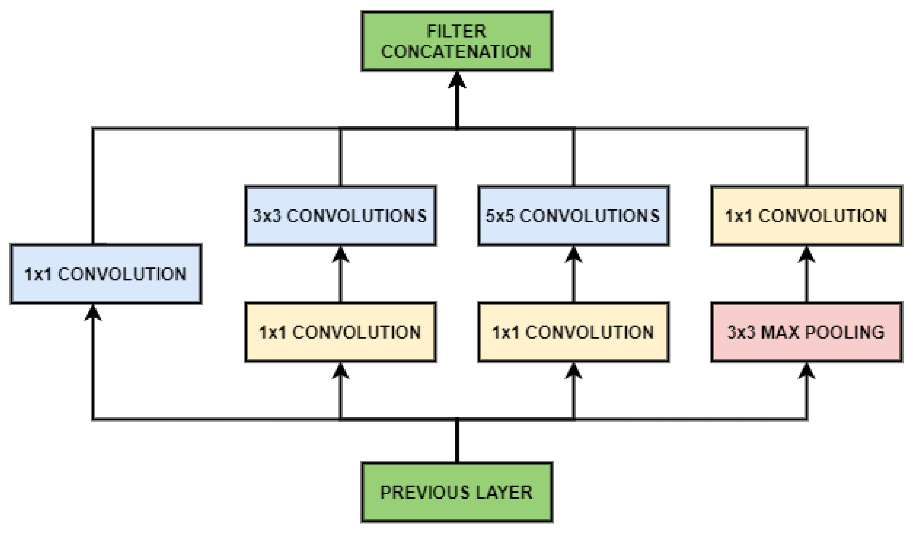
The intuition behind the inception based networks relies on the fact that the correlation within image pixels is local. Taking into consideration local correlations allows for decreasing the number of learning parameters. The first Inception deep CNN was named Inception-v1 [33] and it was introduced as GoogleNet. GoogleNet solves the issue of decreasing the number of learning parameters by including the inception modules in the design of CNN architecture, as shown in Figure 3. The inception module consists of a pooling layer and three convolutional layers with dimensions 1 × 1, 3 × 3, and 5 × 5. Filters with different dimensions are utilized to cover the larger receptive field of each cluster. Outputs from these layers are then concatenated and it represents the module output. Bringing up the batch normalization into the Inception architecture [33,34] resulted in the Inception-v2 model. The third iteration, which was named as Inception-v3 [35], was obtained by additional factorization procedures. This process resulted in three different inception modules: Inception module type 1, obtained by factorization into smaller convolutions; Inception module type 2, reached by factorization into asymmetric convolutions; and, Inception module type 3, which was also introduced to enhance representations with high dimensions.

A CNN architecture based on depthwise separable convolution layers is proposed in [36], presuming that it is a good operation to separate the mapping of cross-channel correlations and spatial correlations in the feature maps of CNN construction. This thesis is a stronger version of the thesis beneath the Inception CNN. For this reason, [36] named the CNN architecture Xception, which means “Extreme Inception”. He proposed improving Inception-based CNNs with the replacement of Inception modules with depthwise separable convolutions. The idea was to construct models by stacking several depthwise separable convolutions. A depthwise separable convolution, which is also known as “separable convolution”, is performed in two steps. The first step is a depthwise convolution, or a spatial convolution implemented separately on every channel of input. The second step is the pointwise convolution. It is a 1 × 1 convolution that conveys to a new channel space the output of the channels obtained with depth-wise convolution.

In order to provide the highest data flow between network layers, the approach [37] connects all CNN layers, with corresponding dimensions of feature maps, straight with each other. The so-called Dense Convolutional Network (DenseNet), attaches each layer to every other layer in a feed-forward manner. For every layer, its inputs are the feature maps of all previous layers. Each layer’s feature maps are conveyed into all succeeding layers, as their input. Figure 4 shows this connectivity pattern schematically. The arrow lines with different colors have the following meaning: they display the input and output of the particular network layer. For example for the second network layer (its feature maps are colored in blue), its inputs are the feature maps of all previous layers and its feature maps are conveyed into all succeeding layers. In Figure 4, BN-RELU-CONV denotes the process of Batch Normalization - Rectified Linear Activation—Convolution. As it can be seen from Figure 4, all of the feature maps go through these operations, and they are concatenated at the end.

When compared to ResNets, the [37] approach does not perform the summation operation on features to lead them afterward into a subsequent layer. On the contrary, it merges features with concatenation.

As can be seen from the schematic layout, the connectivity pattern is dense, so it resulted in the name of CNN Dense Convolutional Network (DenseNet). This CNN contains fewer parameters than other convolutional networks, because the utilization of dense connectivity layout implies that there is no demand to relearn redundant feature maps.

2.2. Linear Learning Rate Decay

The most essential hyperparameters when training a convolutional neural network are the initial learning rate, the number of training epochs, the learning rate schedule, and the regularization method (L2, dropout). Most neural networks are trained with the Stochastic Gradient Descent (SGD) algorithm, which updates the network’s weights W with:

$$W+=\alpha ·gradient$$

(1)

where $\alpha$ is the learning rate, which parameter determines the size of the gradient step. Keeping the learning rate constant during network training might be a good choice in some situations, but more often decreasing the learning rate over time is more advantageous.

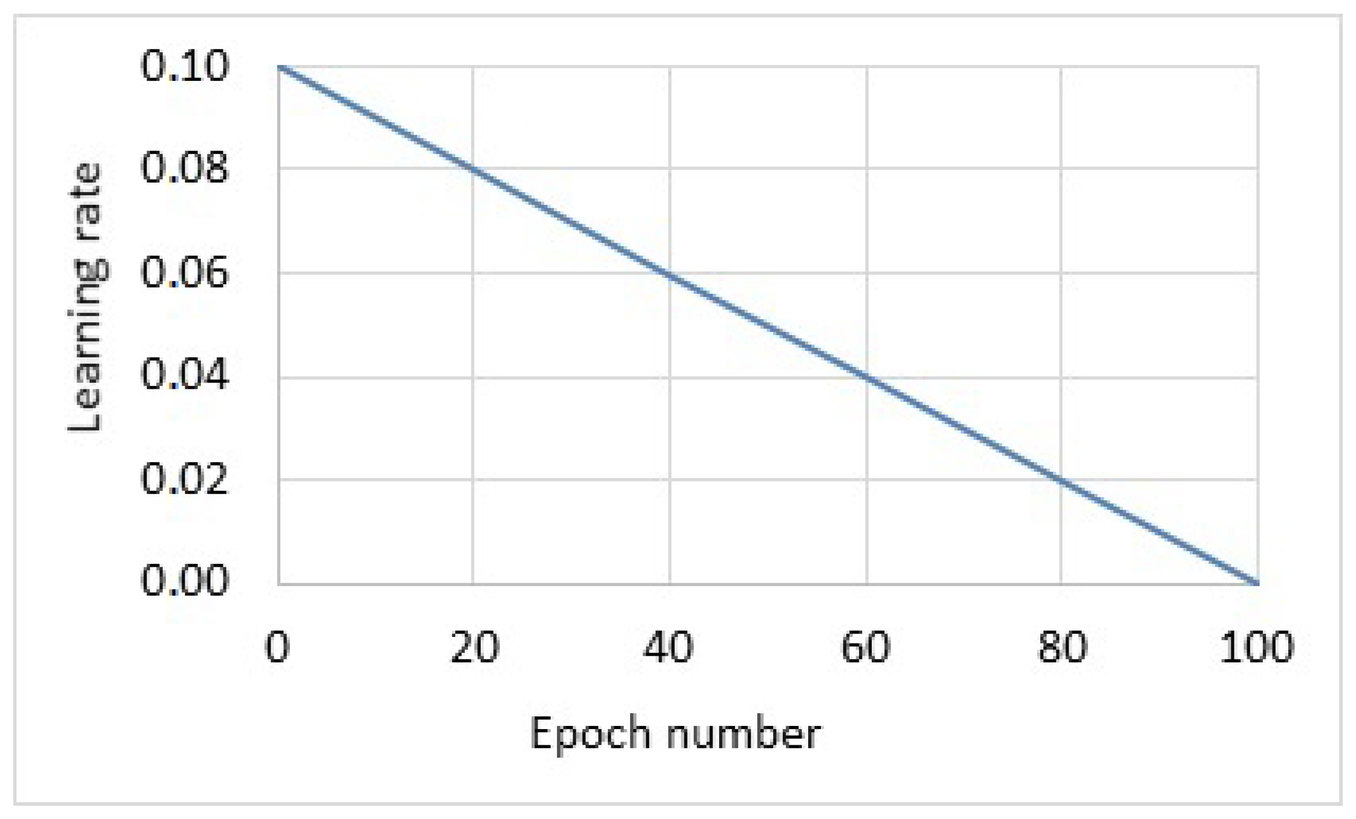
When training CNNs, we are trying to find global minima, local minima, or just an area of the loss function with sufficiently low values. If we have a constant but large learning rate, it will not be possible to reach the desired loss function values. On the contrary, if we decrease our learning rate, our CNNs will be able to descend into more optimal areas of the loss function [38]. In a part of our experiments, we use a linear learning rate decay schedule, which decays our learning rate to zero at the end of the last training epoch, as shown in Figure 5. The learning rate $\alpha$ in every training epoch is given with:

$$\alpha ={\alpha }_1·(1-\frac{E}{E_{max}})$$

(2)

where ${\alpha }_1$ is the initial learning rate, E is the number of the current epoch, and $E_{max}$ is the maximum number of epochs.

All of the CNNs used in our experiments for fine-tuning were originally trained on ImageNet with learning rate schedules: ResNet50 and DenseNet121 with step-based learning rate schedule and Inception V3 and Xception with exponential learning rate schedule.

2.3. Cyclical Learning Rates (Clrs)

Cyclical Learning Rates (CLRs) eliminate the need to identify the optimal value of the initial learning rate and learning rate schedule for CNN training [39]. Despite learning rate schedules, where the learning rate is being constantly decreased, this technique allows for the learning rate to oscillate between reasonable limits. CLRs give us the opportunity to have more freedom in the selection of our initial learning rate. CLRs lead to faster neural network training convergence with fewer hyperparameter updates.

Saddle points are points in the loss function where the gradient is zero, but they do not represent minima or maxima. The authors in [40] found out that the efficiency of CLR methods lies in the loss function topology, and showed that saddle points have a worse impact on minimizing the loss function than poor local minima. One cause for getting stuck in saddle points and global minima can be a learning rate that is too small. CLR methods help to fix this issue adapting the learning rate between a minimum value and a maximum value iteratively. Another reason for the efficiency of CLR methods is that the optimal learning rate is somewhere between the lower and upper bound, so the training is performed with near-optimal learning rates.

There are three main CLR policies: triangular, as shown in Figure 6, triangular2, and exponential range. The triangular policy is a triangular cycle: the learning rate starts from a lower limit, increases the value to the maximum in half a cycle, and then returns to the base value at the end of a cycle. The difference between triangular and triangular2 policy is that the upper bound of a learning rate is decreased in half after every cycle. Training with a triangular2 policy provides more stable training. Exponential range policy, as its name suggests, includes an exponential decay of a maximum learning rate [39].

2.4. Label Smoothing

Label smoothing is a regularization method that allows for a reduction in overfitting and helps CNN architectures to improve their generalization capability. Label smoothing was introduced by [35], and it was shown to boost classification accuracy, adopting a weighted sum of the labels with uniform distribution instead of evaluating the cross-entropy with the “hard” labels from the dataset. “Hard” label assignment corresponds to binary labels: positive for one class and negative for all of the other classes. “Soft” label assignment gives the largest probability to the positive class and very small probability to other classes. Label smoothing is applied to prevent the neural network from being too confident in its prediction. By decreasing the model confidence, we prevent the network training from getting in deep valleys of the loss function [41]. Label smoothing can also be implemented by adding the negative entropy of the softmax output to the negative log-likelihood training objective, weighted by an additional hyperparameter [42,43,44].

The CNN prediction is a function of the activations in the second to last network layer:

$$p_k=\frac{e^{x^T{w}_k}}{{\sum }_{l=1}^L{e}^{x^T{w}_l}}$$

(3)

where $p_k$ is the probability the network classifies to the k-th class, weights and biases of the final network layer are given with $w_k$, x is a vector of activations of the second-last network layer fused with ‘1’ to consider the bias. If we train the network with “hard” labels, we intend to minimize the cross-entropy between the real labels $y_k$ and the neural network’s predictions $p_k$, as follows:

$$H(y,p)=\sum _{k=1}^K-y_{k}log\left(p_k\right)$$

(4)

where $y_k$ is ‘1’ for the correct label and ‘0’ for the others. When train network with label smoothing with parameter $\alpha$, what we minimize is the cross-entropy between the ‘smoothed’ labels $y_k^{LS}$ and the network predictions $p_k$, smoothed labels are given with:

$$y_k^{LS}=y_k(1-\alpha )+\alpha /K$$

(5)

The smoothing technique is used in the proposed method aiming to prevent the neural network from becoming too confident in its predictions and, therefore, increase its robustness and predictive capabilities.

2.5. Datasets

We evaluate our proposed method on two common large-scale remote sensing image datasets, the Aerial Image Dataset (AID) [45] and the NWPU-RESISC45 dataset [46]. A detailed description of the two datasets is given in the following subsections.

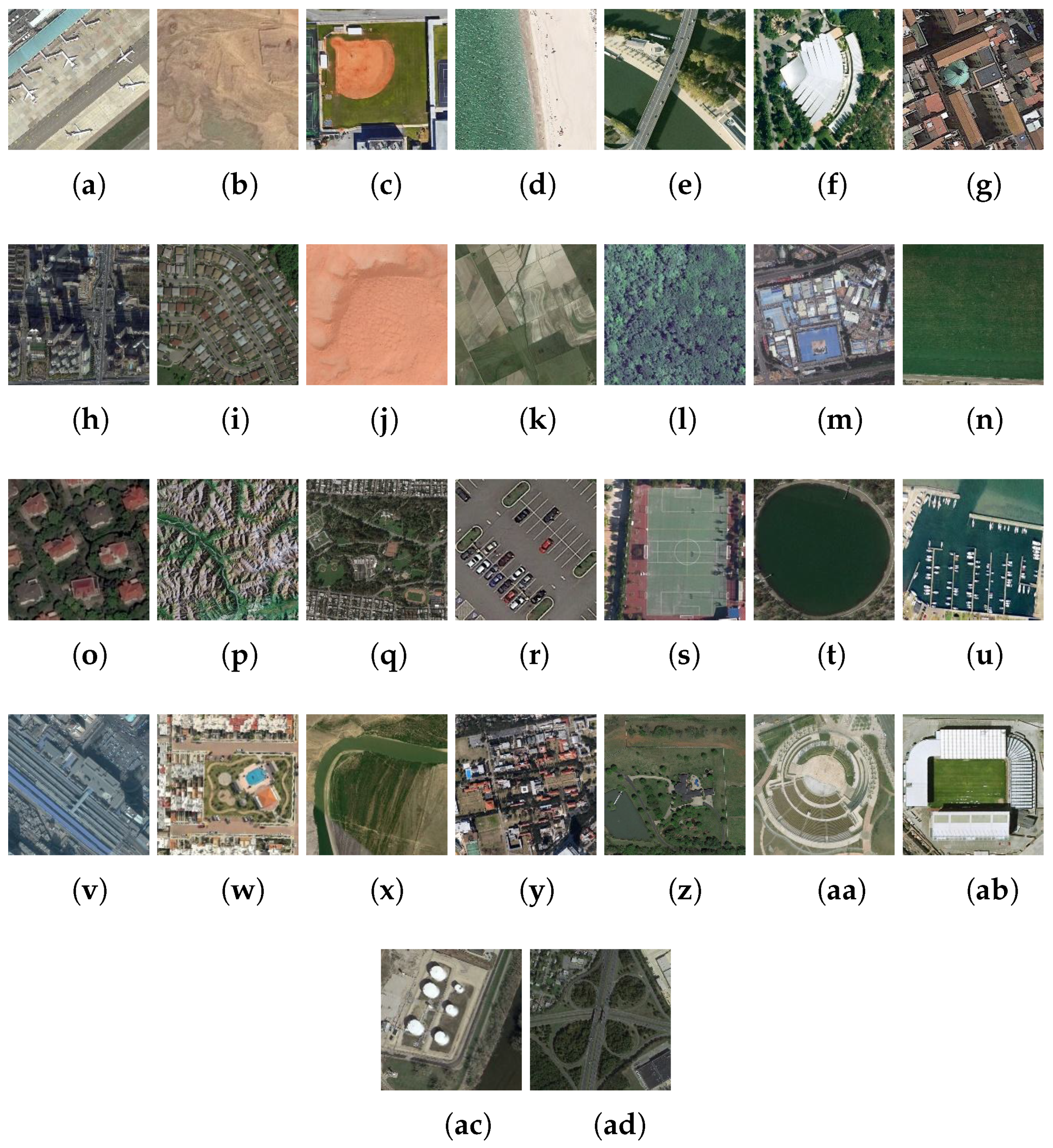
AID consists of about 10,000 remote sensing images with dimensions 600 × 600 pixels, assigned to 30 classes [45]. Images are gathered from Google Earth imagery. They are selected from different continents and countries at different times of the year and weather conditions: mostly from China, Japan, Europe (Germany, England, Italy, and France), and the United States. Images from the AID dataset have a pixel resolution of half a meter. Figure 7 presents sample images of each class.

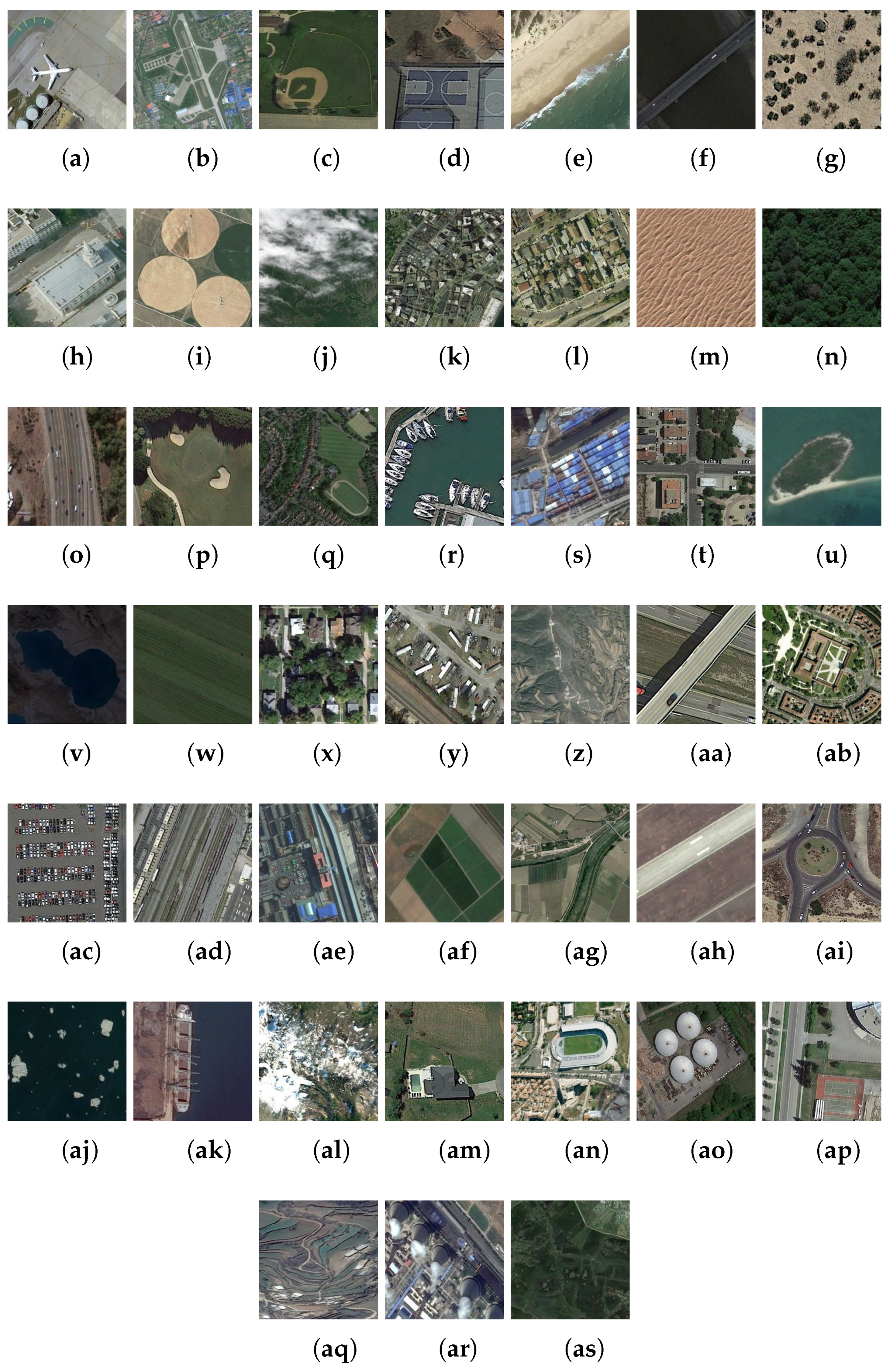
The NWPU-RESISC45 dataset contains images collected from Google Earth imagery. The name of the dataset comes from its creator Northwestern Polytechnical University (NWPU). It consists of 31,500 aerial images split into 45 classes. Each class has 700 images with dimensions 256 × 256 pixels. Except for four classes (island, lake, mountain, and snowberg), which exhibit a smaller spatial resolution, the other classes have spatial resolutions that vary in the range of 30 m–0.2 m. Figure 8 presents sample images of each class.

2.6. Experimental Setup

Our proposed method utilizes fine-tuning as a form of transfer learning, performed with linear decay learning rate schedule and cyclical learning rates, as well as label smoothing for aerial scene classification. In the experiments, we used four CNNs that were pre-trained on the ImageNet dataset: ResNet50, InceptionV3, Xception, and DenseNet121. Fine-tuning was performed through “network surgery”, i.e., we removed the final layers of each of the pre-trained networks after the average pooling layer. After this, we construct a new network head by adding a fully connected layer, dropout, and softmax layer for classification.

As already mentioned, two large-scale remote sensing image datasets are analyzed in our study: AID and NWPU-RESISC45. Images of the datasets were resized according to the requirements of CNN: 224 × 224 for ResNet50 and DenseNet121, and 299 × 299 for InceptionV3 and Xception. The experiments were conducted under the following train/test data split ratios: 50%/50% and 20%/80% for the AID data set and 20%/80% and 10%/90% for NWPU-RESISC45 dataset. The selected split ratios correspond to the ones that were chosen in the related work that we compared our approaches to. The splits were selected randomly and without data stratification.

In-place, data augmentation was used for images from training splits. Data augmentation [47] is a regularization technique that increases the size of the data set, and it almost always results in boosted classification accuracy. Moreover, the label smoothing regularization technique was included in all experiments. Label smoothing was only utilized for the training data splits. It resulted in bigger train loss values compared to the validation loss. On the contrary, label smoothing prevented overfitting and helped our model to generalize better. Overfitting is a common problem when using CNNs with high dimensionality that are pre-trained on datasets of millions of images to solve image classification tasks on datasets that contain a few thousand images.

The first part of the fine-tuning process began with warming-up the new layers of CNN head. New network head layers at the beginning have random initialization of their weights. However, the other network layers after the network surgery have kept their pre-trained weights. Accordingly, it is necessary for the layers of the new network head to start learning the target dataset. During the warming-up process, the only trainable layers were the ones from the new network head; the other network layers were frozen. Warming-up of the new network head was done with a constant learning rate. Fine-tuning of network model continued with Stochastic Gradient Descent (SGD), and, this time, all network layers were “defrosted” for training. Separate experiments were conducted with linear decay of learning rate and for cyclical learning rates with triangular policy. The triangular policy was chosen, since it is the most widely used in the literature, and it yields the highest classification performance compared to other CLR policies. When the linear decay scheduler was applied, the learning rate was steadily decreasing to zero at the end of the last training epoch. The biggest challenge here was to select the initial learning rate, which was chosen to be 1–2 orders of magnitude smaller than the learning rate the original network was trained with. Regarding CLR, we oscillated the learning rate between the maximum and minimum value, assuming that the optimal one is somewhere in the interval. The choice of the lower and upper limit of CLR is not that sensitive as a selection of initial learning rate at a linear decay scheduler. Here, we used a value for step size four or eight times the number of training iterations in the epoch. The number of training epochs was determined in order to contain an integer number of cycles. This is done to keep the idea behind CLRs satisfied: we start from one minimum value of the learning rate, then we go up to the maximum value and, at the end, we return to the starting learning rate. With this action, we have ended one cycle and started all over again.

The second part of our research was dedicated to the evaluation of the classification methods, namely, a softmax classifier and a SVM classifier with linear and Radial Basis Function (RBF) kernel. After fine-tuning of each CNN, we calculated the classification accuracy by the softmax layer, which is a part of the new network head, and it was trained together with all of the other network layers. We used fine-tuned CNNs as feature extractors to compare the capability of the softmax classifier with both types of SVM classifiers. We extracted image features of both remote sensing datasets from the fully-connected layer of fine-tuned neural networks. Afterward, the extracted features were exploited to train the linear as well as RBF SVM and classify the images in the datasets. SVM classification was performed for all datasets splits, adopting both linear decay scheduler and CLRs, and label smoothing in every simulation scenario. All of the simulations were performed on OS Ubuntu 18.04 with Keras v2.2.4. Google’s library TensorFlow v1.12.0 [48], was backend to Keras. The hardware setup was: CPU i7-8700 3.2 GHz and 64 GB RAM. The graphical processor unit was Nvidia GeForce GTX 1080 Ti, with 11 GB of memory and CUDA v9.0 installed on it.

2.7. Evaluation Metrics

In this article, we use two evaluation metrics: Overall Accuracy (OA) and confusion matrix. These evaluation metrics are commonly used for the analysis and comparison of results with other state-of-the-art techniques in classification tasks. OA is calculated as the ratio between the number of correctly classified test images and the entire number of test images. The value of OA is always less than or equal to 1. The confusion matrix is a graphical presentation (table) of the classification accuracy of each class of the dataset. This table shows partial accuracy in each of the image classes. Columns of the confusion matrix depict the predicted classes and the rows show the actual image classes. The classification model should lead to a diagonal confusion matrix (in the ideal case) or a matrix with high values on the diagonal and very low values in other entries. In our experimental setup, the datasets were split into train and test sets. The split was performed without stratification, randomly, and the train/test ratios were selected according to the scales listed in the previous section.

3. Results

3.1. Classification of Aid Dataset

The experimental results of the proposed method for classification of the AID dataset with SVM classifiers are shown in

Table 1. Overall accuracy (%) of the proposed method with a 50%/50% train/test ratio of the AID dataset. The bold text highlights the best accuracy per classifier.

Method	Softmax Classifier	Linear SVM Classifier	RBF SVM Classifier
ResNet50
Linear decay scheduler	$95.62$	$95.88$	$96.12$
Cyclical learning rate	$95.52$	$95.83$	$96.08$
InceptionV3
Linear decay scheduler	$96.41$	96.32	$95.96$
Cyclical learning rate	$95.95$	$95.82$	$96.18$
Xception
Linear decay scheduler	$96.14$	$96.04$	$95.96$
Cyclical learning rate	$96.15$	$95.97$	$96.30$
DenseNet121
Linear decay scheduler	$96.03$	$96.10$	98.03
Cyclical learning rate	$96.21$	$96.3$	$96.60$

and

Table 2. Overall accuracy (%) of the proposed method with a 20%/80% train/test ratio of the AID dataset. The bold text highlights the best accuracy per classifier.

Method	Softmax Classifier	Linear SVM Classifier	RBF SVM Classifier
ResNet50
Linear decay scheduler	$93.06$	$93.09$	$92.98$
Cyclical learning rate	$92.91$	$93.47$	$93.44$
InceptionV3
Linear decay scheduler	$93.7$	$93.32$	93.50
Cyclical learning rate	93.79	$93.41$	93.93
Xception
Linear decay scheduler	$93.67$	$93.29$	94.14
Cyclical learning rate	$93.44$	$93.36$	93.65
DenseNet121
Linear decay scheduler	$93.74$	$93.26$	93.56
Cyclical learning rate	$93.54$	$93.35$	93.58

, for 50%/50% and 20%/80% train/test split ratio, respectively. The above mentioned ratios are common in the literature and they are used in our experiments in order to compare the achieved accuracy with other authors’ research. As can be seen from Table 1, when we use ResNet50 and DenseNet121, which architecture is based on shortcut connections, the linear SVM classifier yields better classification accuracy when compared to a softmax classifier. However, when it comes to the inception based pre-trained CNNs InceptionV3 and Xception, the situation is the opposite, and the classification results are better with the softmax classifier when compared to classification with linear SVM of the extracted features from fine-tuned networks. Analysis of Table 2, which depicts the experimental results for 20%/80% train/test split ratio, shows slightly different outcomes: the softmax classifier works better for InceptionV3, Xception, and DenseNet121, but classification with linear SVM classifier is a better option for ResNet50. One possible explanation for this phenomenon is that SVM performs better with vector data of lower dimensionality. On the contrary, higher dimensionality has less impact on softmax classification. In fact, inspecting the neural network architectures mentioned above, we can notice that the ResNet50 architecture presents a fully connected layer of size 512, whereas Inception-based and DenseNet201 architectures present a fully connected layer of 1024 and 1920 units, respectively.

Comparing the softmax and the RBF SVM classification of the AID dataset shows that the RBF SVM classifier outperforms the softmax classifier for 50%/50% train/test split ratio in all simulation scenarios, except for the InceptionV3 and Xception neural network architectures with linear decay scheduler. For the 20%/80% train/test split ratio of the AID dataset, RBF SVM achieves better classification accuracy than softmax, except for ResNet50, InceptionV3, and DenseNet121 with linear decay scheduler.

Table 3. Overall accuracy (%) of the proposed method compared to reference methods with 50% and 20% of the AID data set as a training set. For our method, we selected the best results obtained for the two training ratios, and report them in bold. Methods are ordered in ascending order by their performance on the 50% training ratio.

Method	50% Training Ratio	20% Training Ratio
GoogleNet+SVM [45]	$86.39$	$83.44$
VGG-VD-16 [45]	$89.64$	$86.59$
CaffeNet [45]	$89.53$	$86.86$
salM3LBP-CLM [49]	$89.76$	$86.92$
MCNNs [50]	$91.80$	/
Fusion by addition [51]	$91.87$	/
X-Net-LF [52]	$92.96$	$90.87$
ARCNet-VGG16 [14]	$93.10$	$88.75$
VGG-16 (fine-tuning) [53]	$93.60$	$89.49$
VGG-16+MSCP [54]	$94.42$	$91.5$
Two-stream fusion [22]	$94.58$	$92.32$
Multilevel fusion [55]	$95.36$	/
GBNet + global Feature [53]	$95.48$	$92.20$
Xception with linear decay scheduler and RBF SVM classifier (proposed)	$95.96$	$94.14$
InceptionV3-CapsNet [56]	$96.32$	$93.79$
EfficientNet-B3-aux [4]	$96.56$	$94.19$
GCFs + LOFs [57]	$96.85$	$92.48$
D-CNNs with VGGNet-16 [12]	$96.89$	$90.82$
Dense-based CNNs + 3D pooling [58]	$97.19$	$95.37$
DenseNet121 with linear decay scheduler and RBF SVM classifier (proposed)	$98.03$	$93.56$

presents a comparison of the proposed method to other state-of-the-art techniques. We achieved the best classification results on the AID dataset with a 50% training set for DenseNet121 with a linear decay scheduler and a RBF SVM classifier, and with a 20% training set for Xception with a linear decay scheduler and a RBF SVM classifier. To the best of our knowledge, our proposed method for 50% training set of AID dataset outperforms all of the other methods in the literature. The standard deviation of achieved classification accuracy of AID dataset is in interval ± (0.1–0.4).

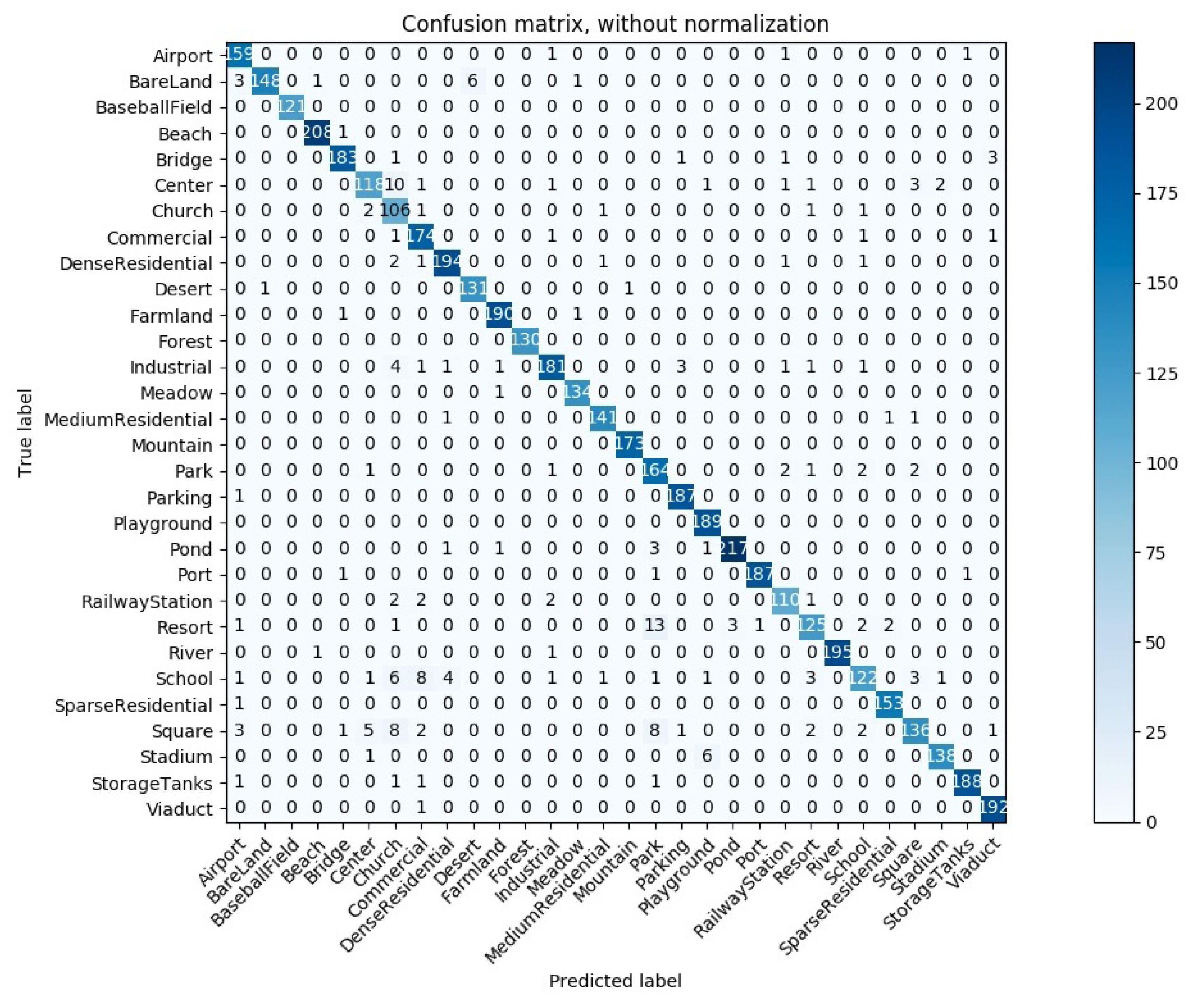
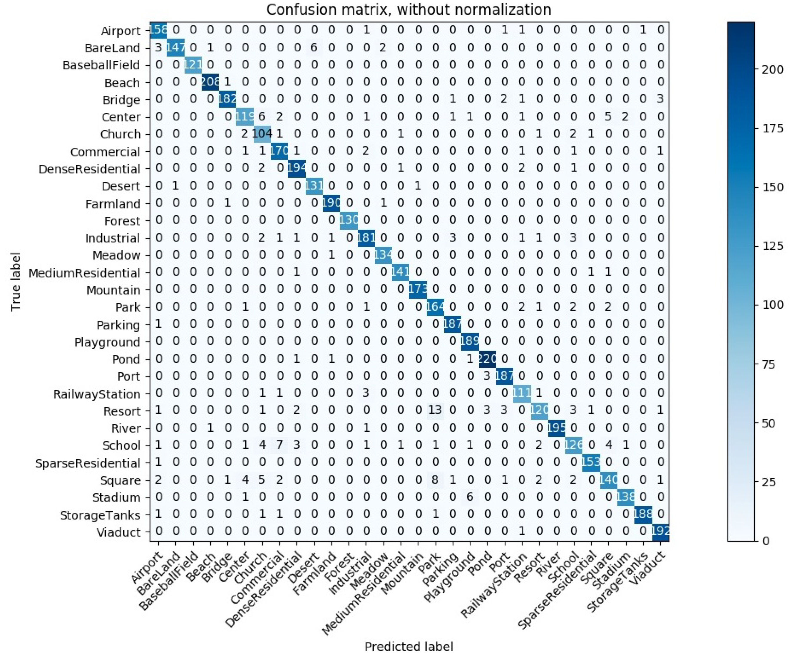
Figure 9 and Figure 10 show the confusion matrices for the AID dataset with a 50%/50% train/test split ratio for ResNet50, linear learning rate decay, and softmax or linear SVM classifier, respectively. Because the classification accuracy achieved with softmax and linear SVM is close, both confusion matrices differ only in the classification outcome for a small number of images.

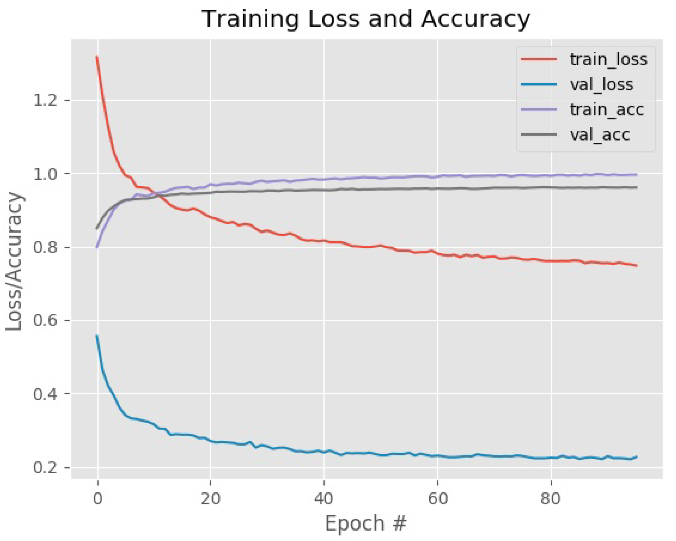
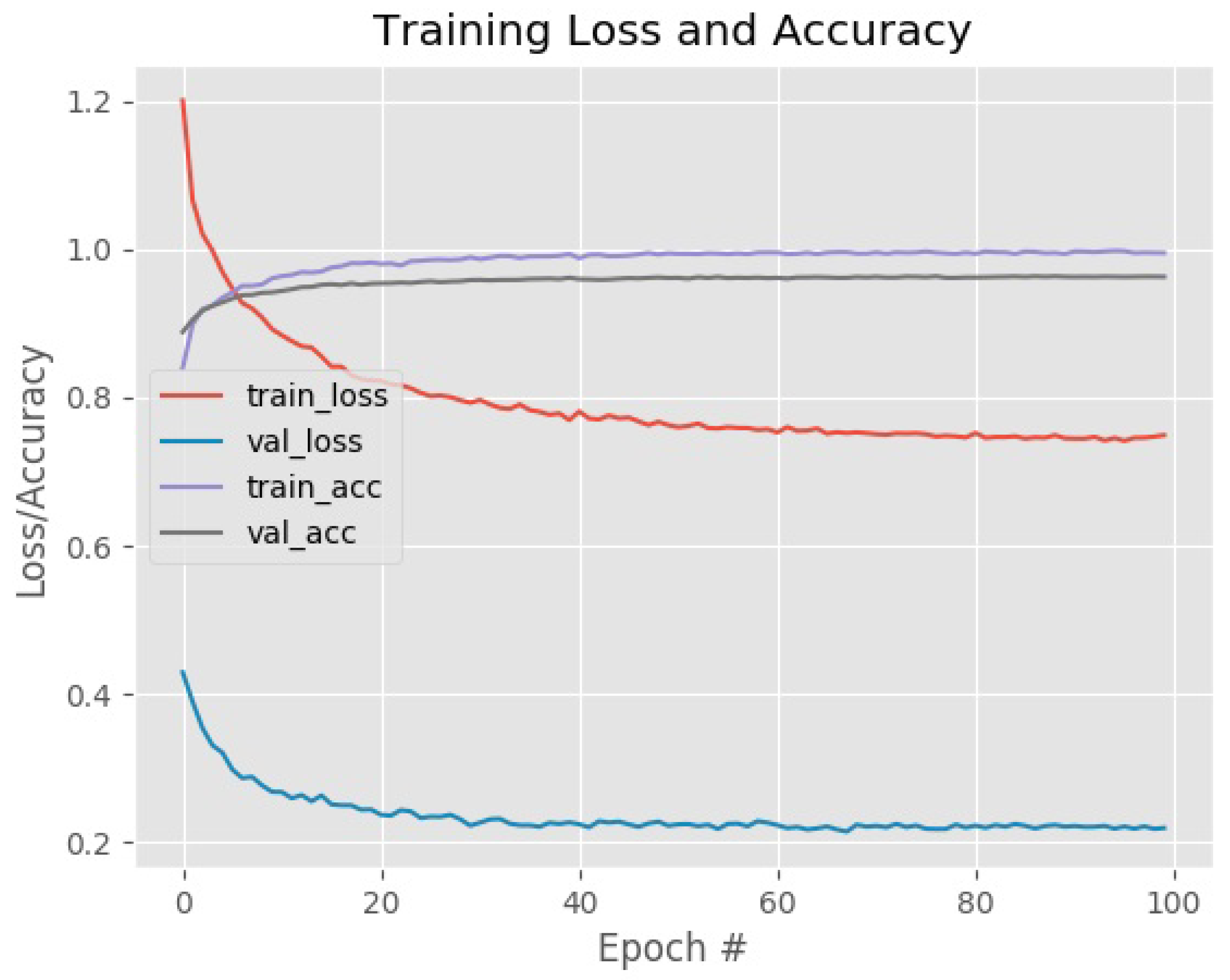
Fine-tuning of Xception with 20% of the AID dataset as a training set for CLR or linear decay learning rate scheduler and the softmax classifier is depicted in Figure 11 and Figure 12, respectively. Two plots show only the fine-tuning of all network layers with the SGD optimizer, but not the warming-up of network head. From the plots, we can see that training with CLR is more stable with characteristic picks on training and validation loss curves, causing some oscillations that are visible as a waved shape. Additionally, it is noticeable that the training loss is more prominent than validation loss on both Figures, because we have applied label smoothing on training labels only.

3.2. Classification of the Nwpu-Resisc45 Data Set

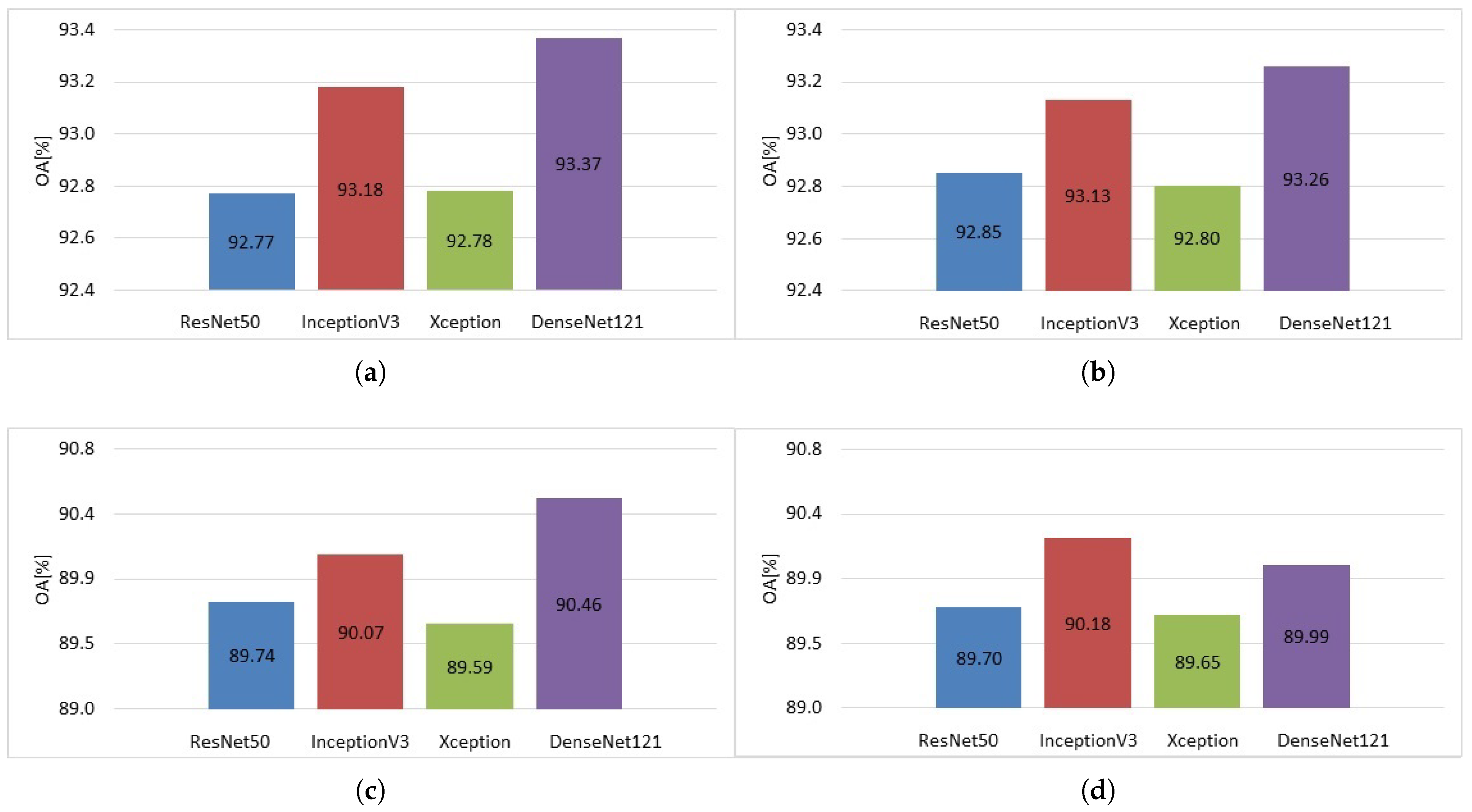
The experimental results of our proposed method with linear and RBF SVM for the NWPU-RESISC45 dataset are displayed in

Table 4. Overall accuracy (%) of the proposed method with 20%/80% train/test ratio of NWPU-RESISC45 data set. The bold text highlights the best accuracy per classifier.

Method	Softmax Classifier	Linear SVM Classifier	RBF SVM Classifier
ResNet50
Linear decay scheduler	$92.35$	$92.77$	$92.89$
Cyclical learning rate	$92.40$	$92.85$	$92.77$
InceptionV3
Linear decay scheduler	$93.07$	$93.18$	$93.35$
Cyclical learning rate	$93.04$	$93.13$	$92.82$
Xception
Linear decay scheduler	$92.63$	$92.78$	$92.72$
Cyclical learning rate	$92.63$	$92.80$	$92.87$
DenseNet121
Linear decay scheduler	$93.16$	93.37	93.60
Cyclical learning rate	$92.98$	$93.26$	$93.55$

and

Table 5. Overall accuracy (%) of the proposed method with a 10%/90% train/test ratio of NWPU-RESISC45 data set. The bold text highlights the best accuracy per classifier.

Method	Softmax Classifier	Linear SVM Classifier	RBF SVM Classifier
ResNet50
Linear decay scheduler	$89.42$	$89.74$	90.03
Cyclical learning rate	$89.20$	$89.70$	89.99
InceptionV3
Linear decay scheduler	$90.16$	$90.07$	90.36
Cyclical learning rate	$90.21$	$90.18$	90.36
Xception
Linear decay scheduler	$89.62$	$89.59$	89.18
Cyclical learning rate	$89.40$	$89.65$	89.67
DenseNet121
Linear decay scheduler	$90.25$	90.46	90.42
Cyclical learning rate	$89.73$	$89.99$	90.11

and Figure 13. Table 4 shows the achieved classification accuracy for a 20%/80% train/test split ratio of the data set. It can be noticed that for linear decay scheduler and as well for CLRs, the linear SVM classifier gives better overall accuracy compared to softmax classifier for all pre-trained CNN. Table 5 shows the obtained classification accuracy for a 10%/90% train/test split ratio for the NWPU-RESISC45 data set. Both train/test split ratios for the analyzed datasets are chosen in order to make experimental comparisons with other studies in the corresponding field of research, which use the same proportions of train/test splits. Here the achieved experimental results are similar to the ones from Table 4. The linear SVM classifier outperforms the softmax classifier in all cases except when we fine-tune the InceptionV3 neural network and Xception with a linear decay scheduler.

Analysing Table 4 and Table 5, we notice that classification with RBF SVM classifier yields better experimental results when compared to softmax classification with the NWPU-RESISC45 dataset. For the 20%/80% train/test split ratio RBF SVM outperforms softmax classification in all simulation scenarios, except for InceptionV3 with cyclical learning rates. For the 10%/90% train/test split ratio, softmax yields better classification results only for Xception with linear decay scheduler.

Table 6. Overall accuracy (%) of the proposed method compared to reference methods with 20% and 10% of NWPU-RESISC45 data set as a training set. For our method, we selected the best results obtained for the two training ratios, and report them in bold. Methods are ordered in ascending order by their performance on the 20% training ratio.

Method	20% Training Ratio	10% Training Ratio
GoogleNet [46]	$78.48$	$76.19$
VGG-16 [46]	$79.79$	$76.47$
AlexNet [46]	$79.85$	$76.69$
Two-stream fusion [15]	$83.16$	$80.22$
BoCF [46]	$84.32$	$82.65$
Fine-tuning AlexNet [46]	$85.16$	$81.22$
Fine-tuning GoogleNet [12]	$86.02$	$82.57$
SAL-TS-Net (Yu et Liu 2018a)	$87.01$	$85.02$
VGG-16+MSCP [51]	$88.93$	$85.33$
Fine-tuning VGG-16 [46]	$90.36$	$87.15$
D-CNNs with VGGNet-16 [12]	$91.89$	$89.22$
Triplet networks [59]	$92.33$	/
Inception-V3-CapsNet [58]	$92.60$	$89.03$
DenseNet121 with linear decay scheduler and linear SVM classifier (proposed)	$93.37$	$90.46$
DenseNet121 with linear decay scheduler and RBF SVM classifier (proposed)	$93.60$	$90.42$
EfficientNet-B3-aux [4]	$93.81$	$91.08$
Dense-based CNNs + 3D pooling [58]	$94.95$	$92.9$

compares the examined techniques with other state-of-the-art methods. Our proposed technique obtained the best classification accuracy with DenseNet121 with a linear decay scheduler and linear SVM classifier for the 10%/90% train/test split ratio of the NWPU-RESISC45 dataset. For the 20%/80% train/test split ratio of NWPU-RESISC45 dataset we achieved the best experimental results with DenseNet121 with a linear decay scheduler and RBF SVM classifier. The standard deviation of achieved classification accuracy of NWPU-RESISC45 dataset is in interval ± (0.1–0.3). From Table 6, it can be concluded that there are methods that outperform our proposed method. One of them uses fine-tuning of EfficientNet-B3 with auxiliary classifier [4]. EfficientNet-B3 yields better top-1 and top-5 classification accuracy on ImageNet data set compared to the pre-trained CNNs utilized in this article, and this is probably the main reason for the better overall accuracy. The results reported in [58] are also better than ours. However, they use multiple fusion of features extracted from dataset images or their parts with different dimensions (scale). Instead, we utilized fine-tuning with one image size according to the pre-trained CNNs requirements.

4. Discussion

We can make several conclusions from our completed simulations and experimental results. All of the presented points, except the last two, refer to research experiments with linear SVM classifier. The last two points refer to cases that include SVM classification with RBF kernel. The main points of this research paper are given, as follows:

• The pre-trained InceptionV3 network yields the highest classification accuracy in transfer learning through fine-tuning for the AID dataset for 50%/50% train/test split ratio and linear SVM classification (Table 1). For the NWPU-RESISC45 dataset, DenseNet121 achieves the best experimental results, but InceptionV3 is the second-best pre-trained CNN. AID dataset images have an original dimension of 600 × 600, and NWPU-RESISC45 dataset images have a dimension of 256 × 256. Each of the pre-trained CNNs requires images with precise dimensions on its input: 299 × 299 for InceptionV3, 224 × 224 for DenseNet121. The achieved sub-optimal results may depend on the cropping of dataset images to the required input dimensions. Taking into consideration the achieved top-one and top-five classification accuracy on the ImageNet dataset, it is somewhat expected that Xception would be the best performing pre-trained CNN, but it is not the case. However, InceptionV3 is right behind Xception according to the achieved results on ImageNet, so it reflects on our research as well.
• Linear learning rate decay scheduler gives better classification accuracy in all experimental scenarios with 50%/50% train/test split for the AID dataset for linear SVM classification. Cyclical Learning Rates (CLRs) are better in cases under 20% training set for the AID data set. Both train/test split ratios of the NWPU-RESISC45 dataset (20%/80% and 10%/90%) have mixed results for linear SVM classification: half of them in favor of linear decay scheduler, half of them in favor of cyclical learning rates. CLRs might be the right solution for experimental scenarios under a smaller ratio of the training set. Neural network fine-tuning with cyclical learning rates resulted in more stable training and, thus, less prone to overfitting compared to training with linear decay scheduler. In our experiments, we used a triangular policy for the CLRs, but it might be an option to use the triangular2 policy. Whichever policy is implemented, it should provide the right balance between stability and accuracy of training.
• In every simulation scenario, we implemented label smoothing with factor = 0.1 as a form of regularization. We combined it with dropout regularization with factor = 0.5. The dropout layer is part of the new network head, and it was placed just before the softmax layer. Regularization techniques or a combination of them are useful to combat overfitting and to improve generalization of the model. Our goal with the proposed method was to boost the classification accuracy of RS dataset images, so we did not perform experimental scenarios without label smoothing.
• Classification accuracy achieved with linear SVM is higher in more cases than the classification accuracy obtained with the softmax layer. Softmax classifier works better for the AID dataset: it yields better experimental results for InceptionV3 and Xception with 50% of the data set as a training set, and for all CNNs, except for ResNet50 with 20% training data set. Linear SVM classifier is a better option for the NWPU-RESISC45 dataset: it outperforms the softmax layer in all cases, except for fine-tuning InceptionV3 for both types of learning rates and Xception with linear decay scheduler and 10% training/test data ratio. We conclude that feature extraction of fine-tuned CNNs yields better classification results than end-to-end training with the softmax layer for classification. It goes in line with information in Table 3 and Table 6, that the best performing method for AID and NWPU-RESISC45 data set classification is based on feature extraction (multiple) and three-dimmensional (3D) pooling of extracted features.
• Performing experimental research into classification of remote sensing datasets with RBF SVM classifiers, shows that it is a superior classification technique compared to softmax classification. For the AID dataset RBF SVM classifier outperforms softmax classification in all cases, except in a few of the simulation scenarios with linear decay scheduler. The situation with NWPU-RESISC45 dataset follows the previous example: from 16 simulation scenarios (for both 20%/80% and 10%/90% train/test split ratios) softmax classifier is better than RBF SVM classifier in only two cases. From Table 1, Table 2, Table 4, and Table 5 it is noticeable that it yields better classification accuracy for each examined dataset in most of the simulation cases.
• Comparing the linear decay scheduler and cyclical learning rate for RBF SVM classification, leads to similar conclusions as for linear SVM classification. The linear decay scheduler shows better experimental results for bigger training sets (50% training set for AID dataset and 20% training set for NWPU-RESISC45 dataset). Cyclical learning rates appear more suitable for aerial scene classification under smaller training sets.

5. Conclusions

In this paper, we presented a fine-tuning method for image classification of large-scale remote sensing datasets. We showed that the adoption of a linear decay learning rate schedule or Cyclical Learning Rates, combined with regularization techniques, like label smoothing, could produce state-of-the-art results in terms of overall accuracy. Summarizing, SVM with linear or RBF kernel presented more accurate results than softmax when using 10% and 20% training data splits. This behavior is expected, since SVM is known to be more robust in the presence of of small training sets [60]. The above discussion is giving us valuable information for researching more competitive methods to provide progress in remote sensing image classification. After this, we suggest the following directions: (1) assess the method with different types of pre-trained CNNs with different types of neural network architectures, (2) include learning rate finder [39] in order to determine optimal boundaries for cyclical learning rates or initial learning rate for linear decay scheduler, and (3) improve the results by fine-tuning only some layers of pre-trained CNNs, in contrast with unfreezing the whole network architecture for training.

References

1. Liang, Y.; Monteiro, S.T.; Saber, E.S. Transfer Learning for High-Resolution Aerial Image Classification. In Proceedings of the IEEE Applied Imagery Pattern Recognition (AIPR) Workshop, Washington, DC, USA, 18–20 October 2016. [Google Scholar]
2. Cheng, G.; Xie, X.; Han, J.; Guo, L.; Xia, G. Remote Sensing Image Scene Classification Meets Deep Learning: Challenges, Methods, Benchmarks, and Opportunities. arXiv 2020, arXiv:2005.01094. [Google Scholar] [CrossRef]
3. Khelifi, L.; Mignotte, M. Deep Learning for Change Detection in Remote Sensing Images: Comprehensive Review and Meta-Analysis. IEEE Access 2020, 8, 126385–126400. [Google Scholar] [CrossRef]
4. Bazi, Y.; Rahhal, M.M.A.; Alhichri, H.; Alajlan, N. Simple Yet Effective Fine-Tuning of Deep CNNs Using an Auxiliary Classification Loss for Remote Sensing Scene Classification. Remote Sens. 2019, 11, 2908. [Google Scholar] [CrossRef] [Green Version]
5. Lu, Y.; Luo, L.; Huang, D.; Wang, Y.; Chen, L. Knowledge Transfer in Vision Recognition. ACM Comput. Surv. 2020, 53, 1–35. [Google Scholar] [CrossRef]
6. Yosinski, J.; Clune, J.; Bengio, Y.; Lipson, H. How transferable are features in deep neural networks? In Proceedings of the Advances in Neural Information Processing Systems 27: Annual Conference on Neural Information Processing Systems 2014, Montreal, QC, Canada, 8–13 December 2014; pp. 3320–3328. [Google Scholar]
7. Razavian, A.S.; Azizpour, H.; Sullivan, J.; Carlsson, S. CNN features off-the-shelf: An astounding baseline for recognition. In Proceedings of the IEEE Conference on Computer Vision and Pattern Recognition Workshops, Columbus, OH, USA, 23–28 June 2014; p. 512519. [Google Scholar]
8. Penatti, O.A.; Nogueira, K.; dos Santos, J.A. Do deep features generalize from everyday objects to remote sensing and aerial scenes domains? In Proceedings of the IEEE Conference on Computer Vision and Pattern Recognition Workshops, Boston, MA, USA, 7–12 June 2015; p. 4451. [Google Scholar]
9. Hu, F.; Xia, G.S.; Hu, J.; Zhang, L. Transferring deep convolutional neural networks for the scene classification of high-resolution remote sensing imagery. Remote Sens. 2015, 7, 14680–14707. [Google Scholar] [CrossRef] [Green Version]
10. Nogueira, K.; Penatti, O.A.; Dos Santos, J.A. Towards Better Exploit. Convolutional Neural Networks Remote Sens. Scene Classification. Pattern Recognit. 2017, 61, 539–556. [Google Scholar] [CrossRef] [Green Version]
11. Sermanet, P.; Eigen, D.; Zhang, X.; Mathieu, M.; Fergus, R.; LeCun, Y. Overfeat: Integrated recognition, localization, and detection using convolutional networks. arXiv 2013, arXiv:1312.6229. [Google Scholar]
12. Cheng, G.; Yang, C.; Yao, X.; Guo, L.; Han, J. When deep learning meets metric learning: Remote sensing image scene classification via learning discriminative CNNs. IEEE Trans. Geosci. Remote Sens. 2018, 56, 2811–2821. [Google Scholar] [CrossRef]
13. Chaib, S.; Liu, H.; Gu, Y.; Yao, H. Deep feature fusion for VHR remote sensing scene classification. IEEE Trans. Geosci. Remote Sens. 2017, 55, 4775–4784. [Google Scholar] [CrossRef]
14. Wang, Q.; Liu, S.; Chanussot, J.; Li, X. Scene classification with recurrent attention of VHR remote sensing images. IEEE Trans. Geosci. Remote Sens. 2018, 99, 1155–1167. [Google Scholar] [CrossRef]
15. Yu, Y.L.; Liu, F.X. Dense connectivity based two-stream deep feature fusion framework for aerial scene classification. Remote Sens. 2018, 10, 1158. [Google Scholar] [CrossRef] [Green Version]
16. Chatfield, K.; Simonyan, K.; Vedaldi, A.; Zisserman, A. Return Devil Details: Delving Deep Convolutional Nets. arXiv 2014, arXiv:1405.3531. [Google Scholar]
17. Chen, Y.; Xu, W.; Zuo, J.; Yang, K. The fire recognition algorithm using dynamic feature fusion and IV-SVM classifier. Clust. Comput. 2018, 2, 7665–7675. [Google Scholar] [CrossRef]
18. Li, R.; Wang, S. Adaptive Graph Convolutional Neural Networks. In Proceedings of the AAAI Conference on Artificial Intelligence, New Orleans, LA, USA, 2–7 February 2018. [Google Scholar]
19. Pio, G.; Ceci, M.; Prisciandaro, F.; Malerba, D. Exploiting causality in gene network reconstruction based on graph embedding. Mach. Learn. 2020, 109, 1231–1279. [Google Scholar] [CrossRef]
20. Corizzo, R.; Ceci, M.; Japkowicz, N. Anomaly Detection and Repair for Accurate Predictions in Geo-distributed Big Data. Big Data Res. 2019, 16, 18–35. [Google Scholar] [CrossRef]
21. Bao, W.; Yue, J.; Rao, Y. A deep learning framework for financial time series using stacked autoencoders and long-short term memory. PLoS ONE 2017, 12, e0180944. [Google Scholar] [CrossRef] [Green Version]
22. Yu, Y.; Liu, F. A two-stream deep fusion framework for high-resolution aerial scene classification. Comput. Intell. Neurosci. 2018, 2018, 13. [Google Scholar] [CrossRef] [Green Version]
23. Corizzo, R.; Ceci, M.; Zdravevski, E.; Japkowicz, N. Scalable auto-encoders for gravitational waves detection from time series data. Expert Syst. Appl. 2020, 151, 113378. [Google Scholar] [CrossRef]
24. Petrovska, B.; Zdravevski, E.; Lameski, P.; Corizzo, R.; Stajduhar, I.; Lerga, J. Deep Learning for Feature Extraction in Remote Sensing: A Case-study of Aerial Scene Classification. Sensors 2020, 14, 3906. [Google Scholar] [CrossRef]
25. Yue, J.; Zhao, W.; Mao, S.; Liu, H. Spectral–spatial classification of hyperspectral images using deep convolutional neural networks. Remote Sens. Lett. 2015, 6, 468–477. [Google Scholar] [CrossRef]
26. Xie, M.; Jean, N.; Burke, M.; Lobell, D.; Ermon, S. Transfer learning from deep features for remote sensing and poverty mapping. arXiv 2015, arXiv:1510.00098. [Google Scholar]
27. Castelluccio, M.; Poggi, G.; Sansone, C.; Verdoliva, L. Land use classification in remote sensing images by convolutional neural networks. arXiv 2015, arXiv:1508.00092. [Google Scholar]
28. Jarrett, K.; Kavukcuoglu, K.; Ranzato, M.; LeCun, Y. What is the best multi-stage architecture for object recognition? In Proceedings of the 2009 IEEE 12th International Conference on Computer Vision, Kyoto, Japan, 27 September–4 October 2009; pp. 2146–2153. [Google Scholar]
29. Larochelle, H.; Bengio, Y.; Louradour, J.; Lamblin, P. Exploring strategies for training deep neural networks. J. Mach. Learn. Res. 2009, 10, 1–40. [Google Scholar]
30. Mignone, P.; Pio, G.; D’Elia, D.; Ceci, M. Exploiting transfer learning for the reconstruction of the human gene regulatory network. Bioinformatics 2019, 36, 1553–1561. [Google Scholar] [CrossRef] [PubMed]
31. Müller, R.; Kornblith, S.; Hinton, G.E. When does label smoothing help? In Proceedings of the Advances in Neural Information Processing Systems 32: Annual Conference on Neural Information Processing Systems 2019, NeurIPS 2019, Vancouver, BC, Canada, 8–14 December 2019; pp. 4696–4705. [Google Scholar]
32. He, K.; Zhang, X.; Ren, S.; Sun, J. Deep residual learning for image recognition. In Proceedings of the IEEE Conference on Computer Vision and Pattern Recognition, Las Vegas, NV, USA, 27–30 June 2016. [Google Scholar]
33. Szegedy, C.; Liu, W.; Jia, Y.; Sermanet, P.; Reed, S.; Anguelov, D.; Erhan, D.; Vanhoucke, V.; Rabinovich, A. Going deeper with convolutions. In Proceedings of the IEEE Conference on Computer Vision and Pattern Recognition, Boston, MA, USA, 7–12 June 2015; p. 19. [Google Scholar]
34. Ioffe, S.; Szegedy, C. Batch Normalization: Accelerating Deep Network Training by Reducing Internal Covariate Shift. arXiv 2015, arXiv:1502.03167. [Google Scholar]
35. Szegedy, C.; Vanhouck, V.; Ioffe, S.; Shlens, J.; Wojna, Z. Rethinking the Inception Architecture for Computer Vision. In Proceedings of the IEEE Conference on Computer Vision and Pattern Recognition, Las Vegas, NV, USA, 26 June–1 July 2016. [Google Scholar]
36. Chollet, F. Xception: Deep Learning with Depthwise Separable Convolutions. arXiv 2017, arXiv:1610.02357. [Google Scholar]
37. Huang, G.; Liu, Z.; van der Maaten, L.; Weinberger, K.Q. Densely Connected Convolutional Networks. In Proceedings of the IEEE Conference on Computer Vision and Pattern Recognition, Salt Lake City, UT, USA, 18–22 June 2018. [Google Scholar]
38. Bengio, Y. Practical Recommendations for Gradient-Based Training of Deep Architectures. In Neural Networks: Tricks of the Trade, 2nd ed.; Springer: Berlin/Heidelberg, Germany, 2012; pp. 437–478. [Google Scholar]
39. Smith, L.N. Cyclical learning rates for training neural networks. In Proceedings of the 2017 IEEE Winter Conference on Applications of Computer Vision (WACV), Santa Rosa, CA, USA, 24–31 March 2017; IEEE: Piscataway, NJ, USA, 2017; pp. 464–472. [Google Scholar]
40. Dauphin, Y.N.; de Vries, H.; Chung, J.; Bengio, Y. Rmsprop and equilibrated adaptive learning rates for non-convex optimization. In Proceedings of the Advances in Neural Information Processing Systems, Montreal, QC, Canada, 7–12 December 2015. [Google Scholar]
41. Müller, R.; Kornblith, S.; Hinton, G. When Does Label Smoothing Help? arXiv 2019, arXiv:1906.02629. [Google Scholar]
42. Pereyra, G.; Tucker, G.; Chorowski, J.; Kaiser, L.; Hinton, G.E. Regularizing Neural Networks by Penalizing Confident Output Distributions. In Proceedings of the 5th International Conference on Learning Representations (ICLR 2017), Toulon, France, 24–26 April 2017. [Google Scholar]
43. Guo, C.; Pleiss, G.; Sun, Y.; Weinberger, K.Q. On Calibration of Modern Neural Networks. In Proceedings of the 34th International Conference on Machine Learning (ICML 2017), Sydney, NSW, Australia, 6–11 August 2017; pp. 1321–1330. [Google Scholar]
44. Goodfellow, I.J.; Bengio, Y.; Courville, A.C. Deep Learning; Adaptive computation and machine learning; MIT Press: Cambridge, MA, USA, 2016. [Google Scholar]
45. Xia, G.; Hu, J.; Hu, F.; Shi, B.; Bai, X.; Zhong, Y.; Zhang, L.; Lu, X. AID: A Benchmark Data Set for Performance Evaluation of Aerial Scene Classification. IEEE Trans. Geosci. Remote Sens. 2017, 55, 3965–3981. [Google Scholar] [CrossRef] [Green Version]
46. Cheng, G.; Li, Z.; Yao, X.; Li, K.; Wei, Z. Remote Sensing Image Scene Classification Using Bag of Convolutional Features. IEEE Geosci. Remote Sens. Lett. 2017, 55, 3965–3981. [Google Scholar] [CrossRef]
47. Shorten, C.; Khoshgoftaar, T.M. A survey on Image Data Augmentation for Deep Learning. J. Big Data 2019, 6, 60. [Google Scholar] [CrossRef]
48. Abadi, M.; Agarwal, A.; Barham, P.; Brevdo, E.; Chen, Z.; Citro, C.; Corrado, G.S.; Davis, A.; Dean, J.; Devin, M. Tensorflow: Large-Scale Machine Learning on Heterogeneous Distributed Systems. arXiv 2016, arXiv:1603.04467. [Google Scholar]
49. Bian, X.; Chen, C.; Tian, L.; Du, Q. Fusing local and global features for high-resolution scene classification. IEEE J. Sel. Top. Appl. Earth Obs. Remote Sens. 2017, 10, 2889–2901. [Google Scholar] [CrossRef]
50. Liu, Y.; Huang, C. Scene classification via triplet networks. IEEE J. Sel. Top. Appl. Earth Obs. Remote Sens. 2018, 11, 220–237. [Google Scholar] [CrossRef]
51. Wang, G.; Fan, B.; Xiang, S.; Pan, C. Aggregating Rich Hierarchical Features for Scene Classfication in Remote Sensing Imagery. IEEE J. Sel. Top. Appl. Earth Obs. Remote Sens. 2017, 10, 4104–4115. [Google Scholar] [CrossRef]
52. Anwer, R.M.; Khan, F.S.; van de Weijer, J.; Molinier, M.; Laaksonen, J. Binary patterns encoded convolutional neural networks for texture recognition and remote sensing scene classification. Isprs J. Photogramm. Remote Sens. 2018, 138, 74–85. [Google Scholar] [CrossRef] [Green Version]
53. Sun, H.; Li, S.; Zheng, X.; Lu, X. Remote Sensing Scene Classification by Gated Bidirectional Network. IEEE Trans. Geosci. Remote Sens. 2019, 58, 82–96. [Google Scholar] [CrossRef]
54. He, N.; Fang, L.; Li, S.; Plaza, A.; Plaza, J. Remote Sensing Scene Classification Using Multilayer Stacked Covariance Pooling. IEEE Trans. Geosci. Remote Sens. 2018, 56, 6899–6910. [Google Scholar] [CrossRef]
55. Yu, Y.; Liu, F. Aerial Scene Classification via Multilevel Fusion Based on Deep Convolutional Neural Networks. IEEE Geosci. Remote Sens. Lett. 2018, 15, 287–291. [Google Scholar] [CrossRef]
56. Zhang, W.; Tang, P.; Zhao, L. Remote Sensing Image Scene Classification Using CNN-CapsNet. Remote Sens. 2019, 11, 494. [Google Scholar] [CrossRef] [Green Version]
57. Zeng, D.; Chen, S.; Chen, B.; Li, S. Improving remote sensing scene classification by integrating global-context and local-object features. Remote Sens. 2018, 10, 734. [Google Scholar] [CrossRef] [Green Version]
58. Zhang, J.; Lu, C.; Li, X.; Kim, H.J.; Wang, J. A full convolutional network based on DenseNet for remote sensing scene classification. Math. Biosci. Eng. 2019, 16, 3345–3367. [Google Scholar] [CrossRef] [PubMed]
59. Liu, Y.; Zhong, Y.; Qin, Q. Scene Classification Based on Multiscale Convolutional Neural Network. IEEE Trans. Geosci. Remote Sens. 2018, 56, 7109–7121. [Google Scholar] [CrossRef] [Green Version]
60. Shao, Y.; Lunetta, R.S. Comparison of support vector machine, neural network, and CART algorithms for the land-cover classiffication using limited training data points. ISPRS J. Photogramm. Remote Sens. 2012, 70, 78–87. [Google Scholar] [CrossRef]
Figure 1. Flowchart of the proposed method.
Applsci 10 05792 g001
Figure 2. Residual block (top) and “bottleneck” block (bottom) of ResNet [32].
Applsci 10 05792 g002
Figure 3. The architecture of a basic inception module [33].
Applsci 10 05792 g003
Figure 4. Densely concatenated convolution pattern [37].
Applsci 10 05792 g004
Figure 5. Linear learning rate decay applied to Convolutional Neural Network (CNN) training of 100 epochs.
Applsci 10 05792 g005
Figure 6. Cyclical learning rate with triangular policy mode.
Applsci 10 05792 g006
Figure 7. Image classes in the AID dataset: (a) airport; (b) bare land; (c) baseball field; (d) beach; (e) bridge; (f) centre; (g) church; (h) commercial; (i) dense residential; (j) desert; (k) farmland; (l) forest; (m) industrial; (n) meadow; (o) medium residential; (p) mountain; (q) park; (r) parking; (s) playground; (t) pond; (u) port; (v) railway station; (w) resort; (x) river; (y) school; (z) sparse residential; (aa) square; (ab) stadium; (ac) storage tanks; (ad) viaduct.
Applsci 10 05792 g007
Figure 8. Image classes in the NWPU-RESISC45 dataset: (a) airplane; (b) airport; (c) baseball diamond; (d) baseball court (e) beach; (f) bridge; (g) chaparral; (h) church; (i) circular farmland; (j) cloud; (k) commercial area; (l) dense residential; (m) desert; (n) forest; (o) freeway; (p) golf course; (q) ground track field; (r) harbour; (s) industrial area; (t) intersection; (u) island; (v) lake; (w) meadow; (x) medium residential; (y) mobile home park; (z) mountain; (aa) overpass; (ab) palace; (ac) parking lot; (ad) railway; (ae) railway station; (af) rectangular farmland; (ag) river; (ah) roundabout; (ai) runway; (aj) sea ice; (ak) ship; (al) snowberg; (am) sparse residential; (an) stadium; (ao) storage tank; (ap) tennis court; (aq) terrace; (ar) thermal power station; (as) wetland.
Applsci 10 05792 g008
Figure 9. Confusion matrix of the proposed method with a 50%/50% train/test ratio of AID data set for ResNet50, linear learning rate decay, and softmax classifier.
Applsci 10 05792 g009
Figure 10. Confusion matrix of the proposed method with a 50%/50% train/test ratio of AID data set for ResNet50, linear learning rate decay, and a linear SVM classifier.
Applsci 10 05792 g010
Figure 11. Training plot of the proposed method with 20% of AID dataset as the training set for Xception, cyclical learning rate, and softmax classifier.
Applsci 10 05792 g011
Figure 12. Training plot of the proposed method with 20% of AID data set as the training set for Xception, linear learning rate decay, and softmax classifier.
Applsci 10 05792 g012
Figure 13. Overall Accuracy over five runs for NWPU-RESISC45 data set with linear SVM classifier and (a) 20%/80% train/test split ratio, linear decay scheduler; (b) 20%/80% train/test split ratio, cyclical learning rates; (c) 10%/90% train/test split ratio, linear decay scheduler; (d) 10%/90% train/test split ratio, cyclical learning rates.
Applsci 10 05792 g013