Object Semantic Grid Mapping with 2D LiDAR and RGB-D Camera for Domestic Robot Navigation

Abstract

Occupied grid maps are sufficient for mobile robots to complete metric navigation tasks in domestic environments. However, they lack semantic information to endow the robots with the ability of social goal selection and human-friendly operation modes. In this paper, we propose an object semantic grid mapping system with 2D Light Detection and Ranging (LiDAR) and RGB-D sensors to solve this problem. At first, we use a laser-based Simultaneous Localization and Mapping (SLAM) to generate an occupied grid map and obtain a robot trajectory. Then, we employ object detection to get an object’s semantics of color images and use joint interpolation to refine camera poses. Based on object detection, depth images, and interpolated poses, we build a point cloud with object instances. To generate object-oriented minimum bounding rectangles, we propose a method for extracting the dominant directions of the room. Furthermore, we build object goal spaces to help the robots select navigation goals conveniently and socially. We have used the Robot@Home dataset to verify the system; the verification results show that our system is effective.

1. Introduction

Robots are the next frontier technology that affect many aspects of our society, including industry [1], transportation [2], and services [3]. In recent years, more and more service robots, such as FABO [4], KeJia [5], and NAO [6], have entered the human living environment to improve people’s quality of life. In order to complete navigation tasks, the robot needs a map to describe its environment. Traditional map representations include metric, topological, and hybrid ones [7]. The metric map uses grids or geometric features of points, lines, or planes to describe the geometric layout of the environment. To achieve an abstract representation of the environment, a topological map models the environment as a graph, in which vertices correspond to places and edges correspond to the paths. Since the metric map has the characteristic of high localization accuracy and topological map of high path-planning efficiency, the hybrid map takes advantage of both to improve the navigation performance.

Based on an occupied grid or hybrid maps, the metric navigation for small or medium-scale environments is relatively mature. However, when it comes to using the robots in the domestic scene, they lack semantic information for users to order them conveniently. For example, the goal point is defined in geometric coordinates, but humans are more inclined to use natural language interaction. Thus, many researchers are committed to building semantic maps, which not only describe the geometric layout but, also, contain the concepts of rooms or objects, to improve human-robot interactions [8].

At present, there is no consensus on the map forms. Some researchers directly add semantic information to the metric map and some combine metric, topological, and concept maps to generate a semantic map with multiple layers [9]. Our ultimate goal is to build a semantic map with multiple layers, which contains a semantic grid layer, a semantic topological layer, and a semantic concept layer, for domestic robot navigation.

An object semantic grid map is an occupied grid map with object semantics. One of its obvious advantages is that the robot does not need to query the semantics on the concept map, which can improve the efficiency of human-robot interactions to a certain extent. Additionally, it provides an important guarantee for building the multi-layer map. For example, using the occupied grid map and a room segmentation method, the room topology can be obtained. Based on the object semantics and the relation of rooms and objects, the concept of rooms can be generated. By abstracting the semantic grid and the semantic topological map, the semantic concept map can be formed. It should be noted that there are many types of objects in the home environment. Our map contains only static objects that can determine the concept of the room. For objects that cannot be modeled on the map, we will implement navigation goal reasoning based on the relationship between objects and objects and between objects and rooms on the concept map.

Simultaneous localization and mapping (SLAM), which can build an environment map and localize a robot at the same time, is usually used to build metric maps [10]. According to different sensors, it is mainly divided into laser-based SLAM and vision-based SLAM. Laser-based SLAM mainly creates occupied grid maps. Representative algorithms include Hector SLAM [11], GMapping [12], Karto SLAM [13], and Cartographer [14]. Vision-based SLAM mainly builds feature maps, including points [15,16], lines [17,18], or planes [19,20].

Some researchers try to add semantic concepts of objects and rooms based on SLAM to improve the ability of robots’ environment understanding. Using machine-learning methods, some directly add room semantic information on the grid map. For example, Mozos et al. [21] added the semantic labels of the scene through supervised learning. The works proposed by Goerke and Braun [22], Brunskill et al. [23], and Friedman et al. [24], use Adaboost, spectral clustering, and random fields of Voronoi, respectively, to generate topological information. Goeddel and Olson [25] used convolutional neural networks (CNNs) to learn sematic place labels. However, these methods only use grid maps to add room information but cannot generate object semantics. Furthermore, they are not easy to get complex room concepts from. However, if we know the object semantics in a room, we can get the room concepts more easily. For example, Fernandez-Chaves et al. [26] employed a Bayesian probabilistic framework to generate room concepts with object detection.

As it is easier to use visual sensors to add semantic information, many methods employ visual SLAM to build semantic maps. One of the key parts of these methods is to get semantic information of the environments. For that, object recognition [27,28], scene recognition [29,30], the database of the geometric model [31,32], and human-robot interactions [33,34], are used to get semantic concepts. With the development of deep-learning technology, the use of object recognition to add semantics has taken the leading position. However, visual semantic SLAM is still in its infancy. Furthermore, visual SLAM has three problems for domestic robot navigation: (1) The generated map is relatively sparse, which is not very useful for the path planning. (2) While visual localization needs a lot of computing resources, domestic robots only have limited ones. (3) Compared with the laser-based method, it is more fragile and not robust enough. Although the robustness of the system can be improved by fusion of the inertial measurement unit (IMU) [35] or robot encoder [36], there are few studies currently using this method to build semantic maps.

In this paper, we propose an object semantic grid mapping system with Light Detection and Ranging (LiDAR) and RGB-D sensors. We take advantage of the mature navigation based on LiDAR sensors and the ease of adding semantic information with RGB-D sensors to build object semantic grid maps. First, we use a laser-based SLAM to create a grid map and obtain the robot trajectory. Then, we employ camera interpolation and object detection to generate an object point cloud. To get object-oriented minimum bounding rectangles (OOMBRs), we detect the dominant directions of the room. Based on the affordance space theory, we build object goal spaces for robot goal point selection conveniently and socially. We verify the system on a home dataset, and the experimental results show the effectiveness of our system.

In summary, the contributions of this paper are as follows:

• An object semantic grid mapping system with 2D LiDAR and RGB-D sensors for domestic robot navigation is proposed.
• A method for extracting the dominant directions of the room to generate OOMBRs for objects is proposed.
• Object goal spaces are created for robot goal point selection conveniently and socially.
• The effectiveness of the system on a home dataset is verified.

The remainder of this paper is organized as follows. The system overview is introduced in Section 2. The front-end and back-end of the system are detailed in Section 3 and Section 4, respectively. Section 5 presents the experimental results and discussion. Finally, Section 6 concludes this paper.

2. System Overview

The proposed system is shown in Figure 1. First, a 2D laser-based SLAM is used to build an occupied grid map and obtain a robot trajectory. Then, an object detection algorithm is employed to detect the semantics of the objects located in the color image of the RGB-D sensor. Based on the timestamp of the image and the robot trajectory, the camera pose is interpolated to obtain a more accurate result. Based on object detection, depth images, and interpolated poses, a point cloud with object semantic information is generated. To more accurately approximate the occupied spaces of objects, the dominant directions of the room are extracted to generate OOMBRs. To make the robot select goal points conveniently and socially, object goal spaces are created. Finally, the object semantic grid map is generated.

We divide the system into two parts: the front-end and the back-end. The front-end is used for data processing, including laser-based SLAM, camera pose interpolation, and object detection. The back-end is used to generate an object semantic grid map, including object point cloud generation, room dominant direction detection, and object goal space generation. The following first introduces the front-end of the system.

3. Front-End

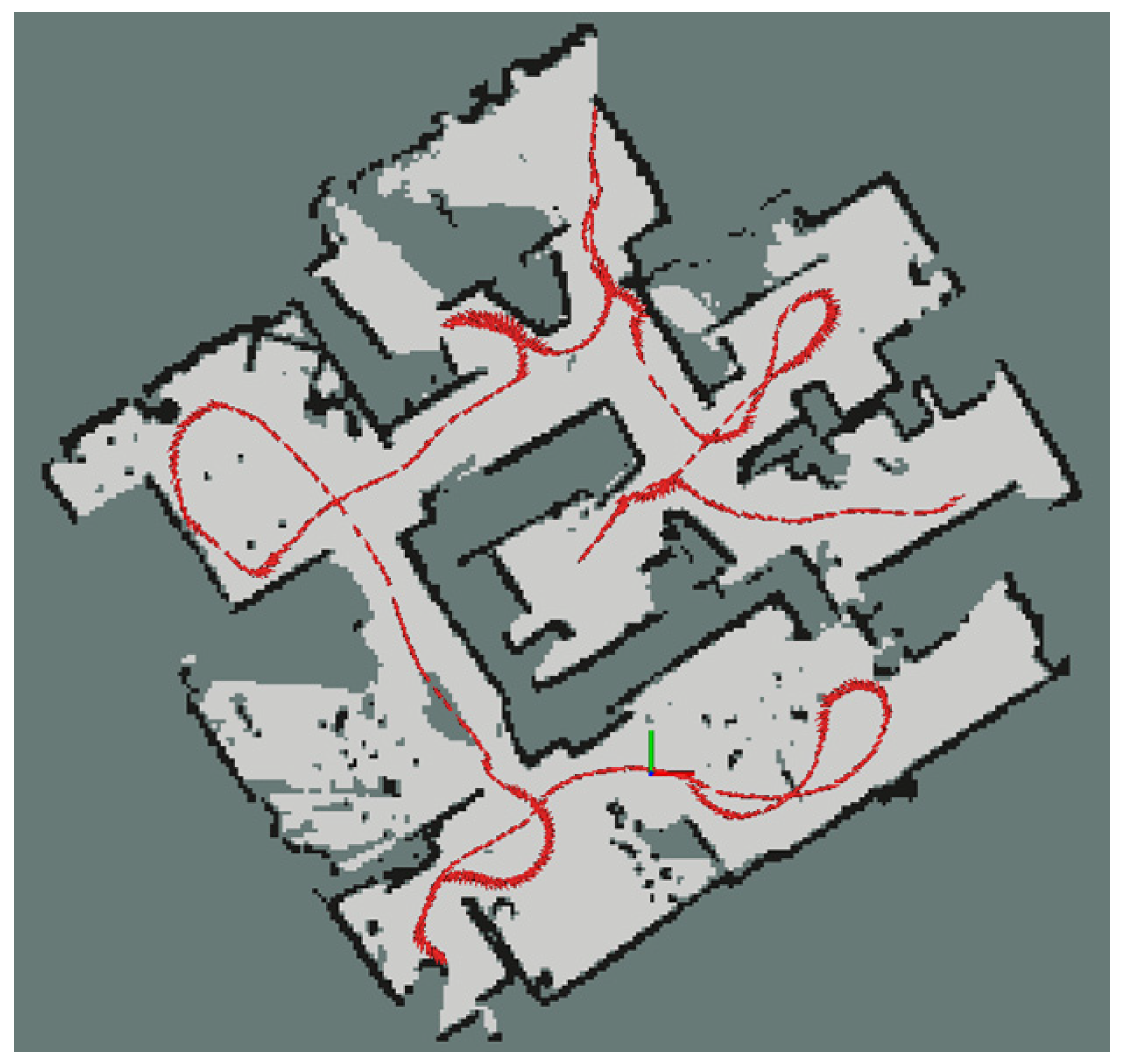
3.1. Laser-Based SLAM

The occupied grid map uses grids to represent the environment. Each grid has three states: occupied, free, or unknown. The occupied indicates the robot cannot pass through while moving; otherwise, it will collide with obstacles. In contrast, the free indicates that there are no obstacles at this position, and the robot can move freely. Finally, the unknown means that the robot failed to detect this grid during the map-building process.

The laser-based SLAM algorithm is always used to build grid maps. The frameworks can be divided into filter-based and graph-based types [10]. Recently, the graph optimization framework has gradually become the mainstream framework, as it can build a more globally consistent map. Cartographer is an open-source SLAM and proposed by Google in 2016. It is state-of-art, due to its high map accuracy, strong robustness, and good system maintainability. We thus use it in the proposed system. As shown in Figure 2, the algorithm can finally generate an occupied grid map and obtain a robot trajectory.

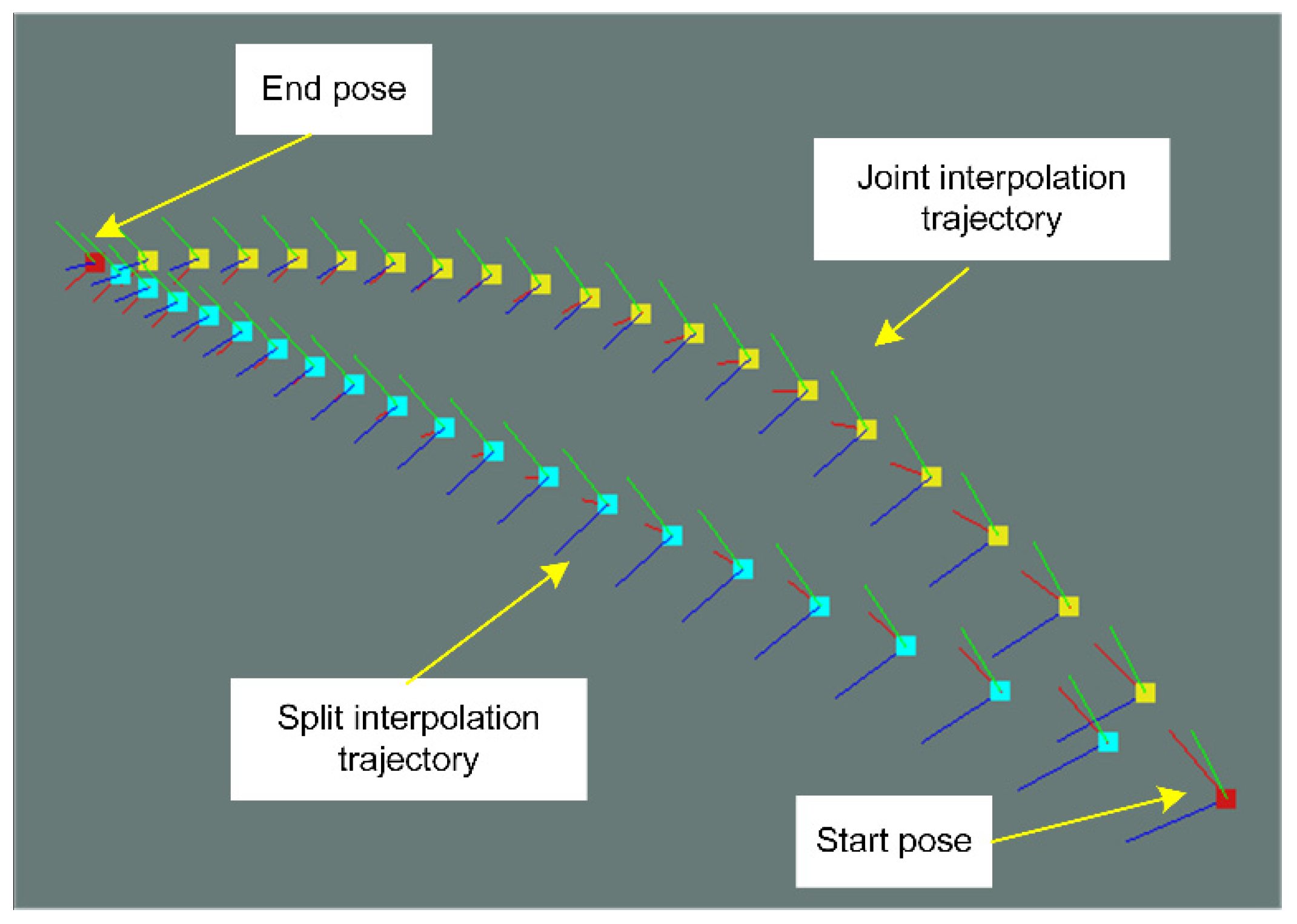
3.2. Camera Pose Interpolation

Camera pose is an important factor that affects the accuracy of the point cloud. Although the Cartographer can estimate the robot pose more accurately, it is difficult to collect synchronized laser and RGB-D sensor data, resulting in the two being not strictly aligned on the timestamp. Interpolation is a method of estimating new data between two discrete points; we thus use it to refine camera poses.

The robot’s pose $Tϵ\mathrm{SE}\left(3\right)$ contains a translation vector $p\in {ℝ}^3$ and a rotation matrix $R\in \mathrm{SO}\left(3\right)$. $\mathrm{SO}\left(3\right)$ and $\mathrm{SE}\left(3\right)$ represent the special orthogonal group and the special Euclidean group, respectively. They are defined as follows:

$$\mathrm{SO}\left(3\right)=\left\{R\in {\mathbb{R}}^{3\times 3}|R{R}^{\mathrm{T}}=I, \det \left(R\right)=+1\right\}.$$

(1)

$$\mathrm{SE}\left(3\right)=\left\{T=\left[\begin{array}{cc}R& \mathit{p}\\ 0^{\mathrm{T}}& 1\end{array}\right]\in {\mathbb{R}}^{4\times 4}|R\in \mathrm{SO}\left(3\right),\mathit{p}\in {\mathbb{R}}^3\right\}.$$

(2)

The method for robot pose interpolation mainly includes two paradigms: the split and the joint [37]. The former first interpolates the position and rotation separately and then composes the results of both to generate a new pose. On the contrary, the latter interpolates the position and rotation simultaneously from the perspective of the special Euclidean group. As shown in Figure 3, they have different interpolation trajectories. We use the joint interpolation to generate camera poses, since the robot trajectory is more in-line with it.

Assuming that the timestamp $t_{\mathrm{c}}$ of an image is between two laser timestamps $t_{\mathrm{l}0}$ and $t_{\mathrm{l}1}$, and the camera poses corresponding to these timestamps are $T_{\mathrm{c}\mathbf{0}}$ and $T_{\mathrm{c}\mathbf{1}}$, then the interpolated camera pose $T_{\mathrm{c}}$ at the time $t_{\mathrm{c}}$ is:

$$T_c=\exp \left(\frac{t_c}{t_{\mathrm{l}1}-t_{\mathrm{l}0}}\log \left(T_{\mathrm{c}1}{T}_{\mathrm{c}0}^{-1}\right)\right)T_{\mathrm{c}0} ,$$

(3)

where $\exp \left(·\right)$ and $\log \left(·\right)$ are the exponential and logarithm maps of $\mathrm{SE}\left(3\right)$.

3.3. Object Detection

At present, object detection based on deep learning has become a mainstream method. The state-of-the-art algorithms, such as YOLO [38], Faster R-CNN [39], and Mask R-CNN [40], are favored by researchers. Using the YOLO and Faster R-CNN, we can obtain the semantic labels, probability values, and bounding rectangles (BRs) of objects. However, the BR is only an approximate representation of the object area—it may include some pixels that do not belong to the object. To solve this problem, Mask R-CNN adds a masked prediction branch on the basis of Faster R-CNN object detection. It can further determine whether the pixels belong to the object and provides more accurate results. We thus use Mask R-CNN to obtain object semantics. Figure 4 shows example results of this algorithm.

The algorithm can detect thousands of objects, so the types need to be limited. We detected six object categories, including bed, couch, sink, toilet, microwave, and oven. These objects are usually not moved frequently and can be used to determine room concepts. For example, a room containing beds is most likely a bedroom, and couches have a large probability of being located in the living room. Considering small objects, such as cups, bowls, and forks, are frequently moved, they are not detected. When the navigation goal points are related to these objects, goal reasoning will be performed according to the instances of the six object categories and room concepts.

4. Back-End

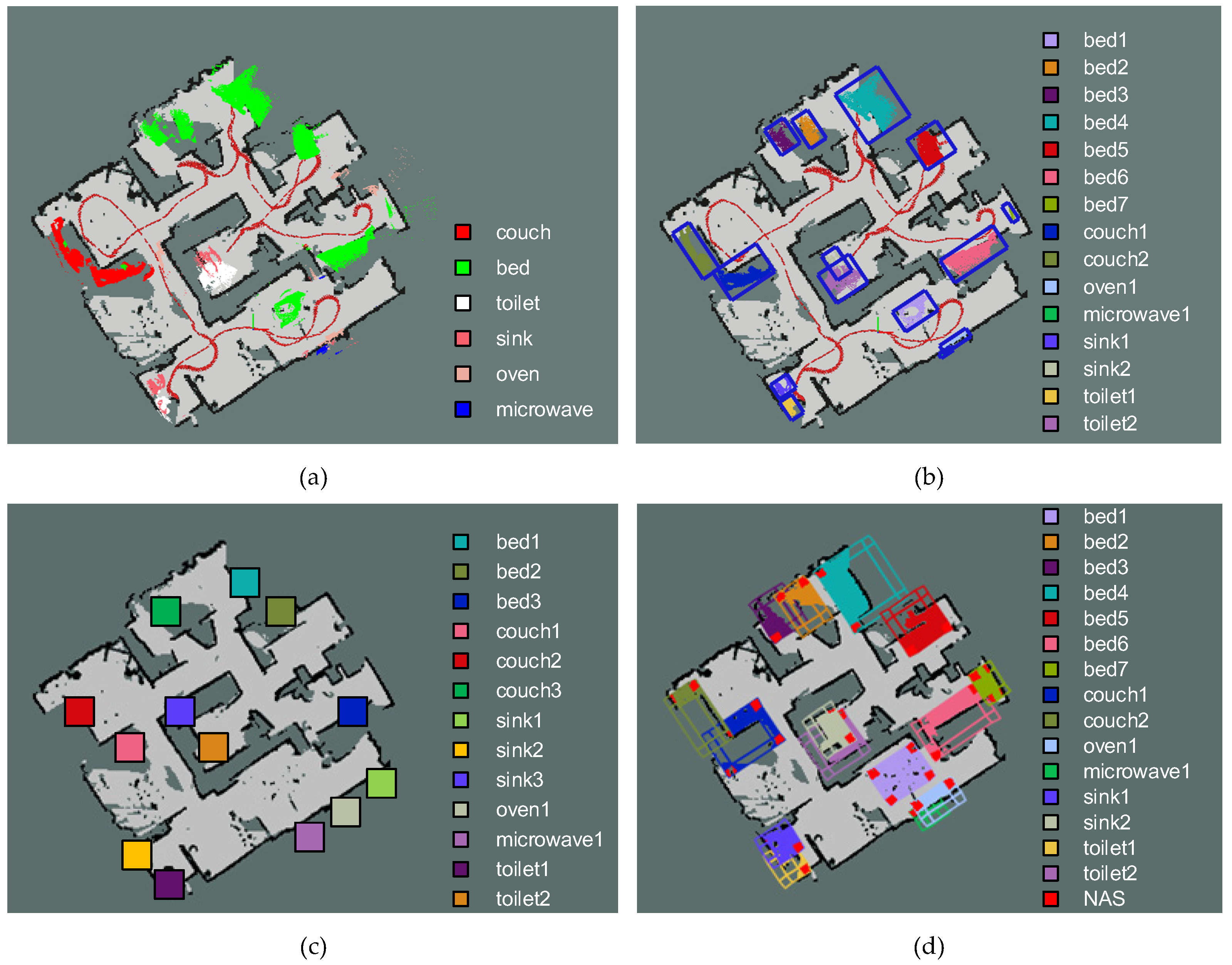
4.1. Object Point Cloud

An object point cloud is a set of 3D points with object semantic labels. We use two steps to generate the cloud—namely, point cloud generation and refinement. The specific contents of each step are introduced below.

The pinhole camera model describes the process of projecting a 3D point in the camera coordinate system to a 2D pixel in the image coordinate system. Defining a point in the camera coordinate system is $X^{\mathrm{c}}={\left[ x^{\mathrm{c}},y^{\mathrm{c}},z^{\mathrm{c}}\right]}^{\mathrm{T}}$; its corresponding pixel u is:

$$u=\left[ \begin{array}{c}u\\ v\\ 1\end{array} \right]=\frac{1}{z^{\mathrm{c}}}\left[ \begin{array}{ccc}{f}_x& 0& c_x\\ 0& f_y& c_y\\ 0& 0& 1\end{array} \right]\left[ \begin{array}{c} x^{\mathrm{c}}\\ y^{\mathrm{c}}\\ z^{\mathrm{c}}\end{array} \right]=\frac{1}{z^{\mathrm{c}}}\mathbf{K}{X}^{\mathrm{c}},$$

(4)

where K is the camera intrinsic and can be obtained by calibration. As shown in Equation (4), depth information is lost during this projection process, resulting in the inability to recover the 3D point by a color image alone. However, an RGB-D camera can obtain both depth image and color image simultaneously. It can directly obtain ($u,v,z^{\mathrm{c}}$). Therefore, based on the RGB-D sensor, the back-projection process of the pinhole camera can generate the 3D point in the camera coordinate system:

$$X^{\mathrm{c}}={\mathrm{z}}^{\mathrm{c}}{K}^{-1}u.$$

(5)

We further use depth and object height constraints to improve the accuracy of the point cloud. The error of the depth image increases with the distance, and the interpolated camera poses may be not very accurate, so we only use the depth value smaller than a certain range.

The object height constraint requires that the 3D object point is within a certain range. We use this constraint to reduce the error results from Mask R-CNN. For example, the model provided by Mask R-CNN is difficult to distinguish between a sink and a chandelier, but the chandelier hangs on the wall and the sink stands on the ground. According to the constraint of the sink, the error results can be removed. Finally, as shown in Figure 5, a 3D point cloud with semantic information can be generated.

Due to sensor noise, inaccurate camera poses, and object detection errors, the point cloud contains many noise and error points. Moreover, the point cloud only includes object semantic labels but does not distinguish different instances. For example, although the environment contains two couches, the point cloud treats them as one. Therefore, the point cloud filter method is used to remove some noise points, and the point cloud segmentation method is employed to obtain different object instances.

Noise points are relatively sparse, while the points within the object are more concentrated. According to this characteristic, we use the statistical filter to remove some noise points [41]. This method assumes that the average distance between a point and its k neighbors follows a Gaussian distribution, then calculates the mean and standard deviation of the distribution, and, finally, takes the points outside the standard deviation as noise points and removes them.

To distinguish different objects with the same semantic label, the Euclidean cluster segmentation is adopted to generate object instances [42]. This method first randomly selects a point in the point cloud and simultaneously generates a new instance, then calculates the nearest neighbors that meets the Euclidean distance threshold and adds them to the instance. Repeat this process until no neighbors can be added to the instance to complete the instance segmentation. At last, repeat the aforementioned process for the remaining point clouds, until all points have an instance label.

Finally, we use the instance minimum number constraint to further refine the object points. In other words, the object instances whose numbers do not satisfy this constraint are removed. Through the above point cloud refinement methods, the generated object point cloud is shown in Figure 6.

4.2. Room Dominant Direction Detection

Although the filtered and instantiated point cloud can better approximate the object positions, due to the influence of the robot trajectory or the installation position of the camera, the robot may not be able to completely observe an object. In other words, the robot can only observe part of the object. To better represent the objects, the minimum bounding box (MBB) is used to determine the approximate shape of the objects.

MBB mainly includes axis-aligned, arbitrarily oriented, and object-oriented forms. The object-oriented means that the box orientation is the same as the local coordinate system of the object. As it can better represent the object and the grid map as a two-dimensional map, we use OOMBR to describe all instances.

The domestic floor plan is usually a rectangular layout, as it has the advantages of simple structure, a high indoor effective area utilization rate, and easy construction. Defining the two directions, which are parallel to the two edges of the rectangle, are the dominant directions of the room. Furthermore, considering that most objects are placed parallel to the dominant directions, we define the object local coordinate axes parallel to them.

Aiming at the rectangular layout, the dominant directions can be extracted by means of line length and direction statistics. While the line detection algorithm needs a binary image, the occupied grid map has three states. To convert the grid map to a binary image, the free grids are regarded as the image foreground, and the unknown and occupied grids are used as the image background. Based on the binary image, we can detect the line segments. In the Cartesian coordinate system, the general equation of a straight line is:

$$ax+by+c=0.$$

(6)

The traditional Hough transform turns a point in the Cartesian coordinate system into a curve in the Hough space:

$$\rho =x\cos \theta +y\sin \theta ,$$

(7)

where $\rho$ is the distance from the origin to the line, and $\theta$ is the angle between the perpendicular line and the x-axis. The parameters can be determined by voting. However, this method cannot obtain the coordinates of the endpoints of the line segments. Cumulative probability Hough line detection can help to obtain them. While reducing the accumulation space, the coordinates of the endpoints of the line segments can also be obtained. Therefore, we use a four-tuple $(P_{\mathrm{s}}, P_{\mathrm{e}},L,l)$ to describe the line segment parameters. Assuming the points of a line segment are $P_{\mathrm{s}}={\left[x_{\mathrm{s}}, y_{\mathrm{s}}\right]}^{\mathrm{T}}$ and $P_{\mathrm{e}}={\left[x_{\mathrm{e}}, y_{\mathrm{e}}\right]}^{\mathrm{T}}$, the straight line parameters L and line segment length l are:

$$L={\left[\mathrm{a},\mathrm{b},\mathrm{c}\right]}^{\mathrm{T}}={\left[P_s^{\mathrm{T}},1\right]}^{\mathrm{T}}\times {\left[P_{\mathrm{e}}^{\mathrm{T}},1\right]}^{\mathrm{T}}.$$

(8)

$$l=||P_s-P_e{||}_2.$$

(9)

When determining the dominant direction of the room, we take the cumulative line length in the same direction as the number of votes. However, some of the obtained line segments belong to the same straight line but are extracted as two line segments with overlapping parts, as shown in Figure 7.

Although, by adjusting the algorithm thresholds, we can reduce this situation. However, in order to reduce the sensitivity of thresholds and improve the detection accuracy of the dominant directions, we use the direction, distance, and coincidence constraints to detect and merge these line segments. Suppose the points of the first line segment are $P_{\mathrm{s}1}={\left[x_{\mathrm{s}1}, y_{\mathrm{s}1}\right]}^{\mathrm{T}}$ and $P_{\mathrm{e}1}={\left[x_{\mathrm{e}1}, y_{\mathrm{e}1}\right]}^{\mathrm{T}}$, and the second line segment are $P_{\mathrm{s}1}={\left[x_{\mathrm{s}1}, y_{\mathrm{s}1}\right]}^{\mathrm{T}}$ and $P_{\mathrm{e}1}={\left[x_{\mathrm{e}1}, y_{\mathrm{e}1}\right]}^{\mathrm{T}}$, the direction constraint requires the angle between the two line segments to be less than the angle threshold ${\delta }_{\varphi }$:

$$\mathrm{acos}\left(\frac{a1a2+b1b2}{\sqrt{a_1^2+b_1^2}\sqrt{a_2^2+b_2^2}}\right)<{\delta }_{\varphi }.$$

(10)

The distance constraint requires that the distance from the first segment points to the second line be smaller than the distance threshold ${\delta }_{\mathrm{d}}$:

$$\frac{|x_{\mathrm{s}1}{a}_2+y_{\mathrm{s}1}{b}_2+c_2\left|+|x_{\mathrm{e}1}{a}_2+y_{\mathrm{e}1}{b}_2+c_2\right|}{2\sqrt{\left(a_2^2+b_2^2\right)}}<{\delta }_{\mathrm{d}}.$$

(11)

The coincidence constraint requires the distance between the midpoints $P_{\mathrm{c}1}$ and $P_{\mathrm{c}2}$ of the line segments be less than the sum of the half-lengths of the line segments:

$$||P_{\mathrm{c}1}-P_{\mathrm{c}2}{||}_2<\frac{1}{2}\left(l_1+l_2\right).$$

(12)

The segment merging method is shown in Figure 8. Based on the first line segment, the projection points of the second line segment are calculated. At last, the points and the first line segment length are recalculated as the merge result.

To count the length of line segments, the directions of all line segments are used as the vote box, the direction constraint threshold is regarded as the box width, and the cumulative length of each direction is the number of votes. The voting result is calculated as shown in Figure 9. The dominant directions of the room ${\varphi }_{\mathrm{m}1}$ and ${\varphi }_{\mathrm{m}2}$ are:

$${\varphi }_{\mathrm{m}1}=\underset{{\varphi }_i}{\mathrm{argmax}}\left\{l\left({\varphi }_i\right)\right\}.$$

(13)

$${\varphi }_{\mathrm{m}2}=\underset{{\varphi }_i}{\mathrm{argmin}}\{\left|{\varphi }_i-{\varphi }_{\mathrm{m}1}\right|-\frac{\pi }{2}|\}.$$

(14)

4.3. Object Goal Space Generation

The dominant direction ${\varphi }_{\mathrm{m}1}$ is used as the orientation of the object. Let us assume that a point $P_i={\left[x_i,y_i,z_i\right]}^{\mathrm{T}}$ belongs to an object instance. According to the dominant direction, the rotated point $P_i^{\prime }$ can be computed as follows:

$$P_i^{\prime }=R\left(-{\varphi }_{\mathrm{m}1}\right)P_i.$$

(15)

Then, the MBR can be computed as follows:

$$\{\begin{array}{c}{x}_{\min }^{\prime }=\min \left\{x_i\right\}\\ y_{\min }^{\prime }=\min \left\{y_i\right\}\\ \begin{array}{c}{x}_{\max }^{\prime }=\max \left\{x_i\right\}\\ y_{\max }^{\prime }=\max \left\{y_i\right\}\end{array}\end{array},$$

(16)

$$\{\begin{array}{c}{P}_{\mathrm{ld}}^{\prime }={\left[x_{\min }^{\prime }, y_{\min }^{\prime },1\right]}^{\mathrm{T}}\\ P_{\mathrm{lu}}^{\prime }={\left[x_{\min }^{\prime },y_{\max }^{\prime },1\right]}^{\mathrm{T}}\\ \begin{array}{c}{P}_{\mathrm{rd}}^{\prime }={\left[x_{\max }^{\prime },y_{\min }^{\prime },1\right]}^{\mathrm{T}}\\ P_{\mathrm{ru}}^{\prime }={\left[x_{\max }^{\prime },y_{\max }^{\prime },1\right]}^{\mathrm{T}}\end{array}\end{array},$$

(17)

where $P_{\mathrm{ld}}^{\prime }$ is the lower left point of the rectangle, $P_{\mathrm{ld}}^{\prime }$ is the upper left, $P_{\mathrm{rd}}^{\prime }$ is the lower right, and $P_{\mathrm{ru}}^{\prime }$ is the upper right. Then, we transform the rectangle in the rotated coordinate system to the map coordinate system:

$$\{\begin{array}{c}{P}_{\mathrm{ld}}=R\left(-{\varphi }_{\mathrm{m}1}\right) P_{\mathrm{ld}}^{\prime }\\ P_{\mathrm{lu}}=R\left(-{\varphi }_{\mathrm{m}1}\right) P_{\mathrm{lu}}^{\prime }\\ \begin{array}{c}{P}_{\mathrm{rd}}=R\left(-{\varphi }_{\mathrm{m}1}\right) P_{\mathrm{rd}}^{\prime }\\ P_{\mathrm{ru}}=R\left(-{\varphi }_{\mathrm{m}1}\right) P_{\mathrm{ru}}^{\prime }\end{array}\end{array}.$$

(18)

Based on the four vertex points of the rectangle, the OOMBR can be generated, as shown in Figure 10.

The navigation goal point is located on a free grid, but the object is located on the occupied or unknown grids. In order to help the robot select goals and make its behavior more in-line with social norms, the object goal space is established. It describes the affordance and nonaffordance space (NAS) of an object. According to the definition in [43], affordance space is related to human activities and is a social space provided by the environment, which is of great significance to realize the navigation behavior accepted by humans. For example, Figure 11a defines the affordance space for a couch, and Figure 11b shows that a FABO robot is in this space. The rationality of this goal needs further discussion. If a human orders the robot to take the cushion on the couch to the bedroom, the point is reasonable, as it is convenient for the robot to execute the next action. On the contrary, if the human just orders the robot to stop nearby the couch, the point is unreasonable, as the affordance space is the potential space for human activities. When people want to sit down, the robot will become an obstacle. Therefore, the robot should stop in the nonaffordance space, in this case.

To formally define these spaces, we first introduce the concepts of 4-connected and 8-connected pixels. The 4-connected pixels are shown in Figure 12a and are defined as follows:

$${\mathcal{N}}_4\left(i,j\right)=\left\{\left(i,j-1\right),\left(i-1,j\right),\left(i,j+1\right),\left(i+1,j\right)\right\}.$$

(19)

The 8-connected pixels are shown in Figure 12b and are defined as follows:

$${\mathcal{N}}_8\left(i,j\right)={\mathcal{N}}_4\left(i,j\right)\cup \left\{\left(i-1,j-1\right),\left(i-1,j+1\right),\left(i+1,j-1\right),\left(i+1,j+1\right)\right\}.$$

(20)

The theoretical model of the goal space is shown in Figure 12c. Similar to the definition of the pixel neighborhoods, the rectangles of the four neighborhoods of the BRs are the theoretical affordance space ${\mathcal{N}}_{\mathrm{a}}^{\prime }\left(i,j\right)$. The rectangles belonging to the eight neighborhoods but not the four neighborhoods are the theoretical nonaffordance space ${\mathcal{N}}_{\mathrm{na}}^{\prime }\left(i,j\right)$:

$$\{\begin{array}{c}{\mathcal{N}}_{\mathrm{a}}^{\prime }\left(i,j\right)={\mathcal{N}}_4\left(i,j\right)\\ {\mathcal{N}}_{\mathrm{na}}^{\prime }\left(i,j\right)={\mathcal{N}}_8\left(i,j\right)-{\mathcal{N}}_4\left(i,j\right)\end{array}.$$

(21)

Assuming the width of a BR is $l_w$, and the height is $l_h$. The affordance space contains four rectangles. One edge length of each rectangle is $l_e,$ and the other is $l_w$ or $l_h$. The nonaffordance space is four squares with the edge length $l_e$:

$$l_e=s_r{l}_r.$$

(22)

where $s_r$ is the safety factor, and $l_r$ is the radius of the robot circumscribed circle.

There are two shortcomings in the theoretical model: (1) It does not consider the uncertainty of the BR of the object. Therefore, it may contain free grids. (2) The real affordance and nonaffordance spaces are a subset of the theoretical ones. For example, the couch has only one rectangle in Figure 11a. We use the grid map to partially solve this problem. For the former, we also consider the free grids in the BR as affordance space; for the latter, we use the occupied and unknown girds to remove some rectangles. Therefore, the real affordance ${\mathcal{N}}_{\mathrm{a}}\left(i,j\right)$ and nonaffordance spaces and ${\mathcal{N}}_{\mathrm{na}}\left(i,j\right)$ are:

$$\{\begin{array}{c}{\mathcal{N}}_{\mathrm{a}}\left(i,j\right)=\left\{{\mathcal{N}}_{\mathrm{a}}^{\prime }\left(i,j\right)\cup \mathcal{B}\left(i,j\right)\right\}\cap \mathcal{F}\\ {\mathcal{N}}_{\mathrm{na}}\left(i,j\right)={\mathcal{N}}_{\mathrm{na}}^{\prime }\left(i,j\right)\cap \mathcal{F}\end{array},$$

(23)

where $\mathcal{B}\left(i,j\right)$ is the grid set of the BR, and $\mathcal{F}$ is the free grid set of the map. Based on the above method, we build the object semantic grid map, as shown in Figure 13.

5. Experimental Results and Discussion

5.1. Experimental Setup

Currently, the academic community has not established a unified standard for the evaluation of semantic maps. Although absolute and relative trajectory errors are usually used to evaluate the algorithm in the field of SLAM, the state-of-the-art can achieve centimeter accuracy in small and medium-scale scenes [44]. For domestic robot navigation, further comparison of the trajectory accuracy is of little practical significance. This evaluation method is more in-line with the needs of 3D reconstruction, virtual reality (VR), augmented reality (AR), and other fields. If we consider how humans are navigating, we can apply this approach to the robot’s path planning. When humans are navigating, they usually do not need to reach the accurate goal position but only need to reach the approximate position near an object and then carry out refined operations. Similar to if the robot can navigate to an object and then use the object to establish a reference coordinate system. This approach to path planning can improve a robot’s overall completion of operation tasks. Using this method may be more practical than requiring the robot to further build a very accurate map [45].

To summarize, for the following considerations, we do not evaluate the accuracy of robots’ trajectories and objects’ poses: (1) the current laser SLAM algorithm can meet the navigation accuracy requirements for small and medium-scale domestic environments. (2) Unlike AR and VR application scenarios, the robot does not need very accurate object poses when performing navigation tasks.

We use precision and the recall of object instantiation to evaluate object semantic gird maps. Supposedly the number of correctly instantiated objects, which have the correct semantic labels and their position errors are not very obvious, is $N_{\mathrm{cins}}$, the number of instantiated objects on the map is $N_{\mathrm{ins}}$, and the number of objects in the environment is $N_{\mathrm{gtins}}$; then, the precision $P_{\mathrm{ins}}$ and recall $R_{\mathrm{ins}}$ of object instantiation are defined as follows:

$$P_{\mathrm{ins}}=\frac{N_{\mathrm{cins}}}{N_{\mathrm{ins}}},$$

(24)

$$R_{\mathrm{ins}}=\frac{N_{\mathrm{cins}}}{N_{\mathrm{gtins}}}.$$

(25)

For object detection, we employ an instance of Mask R-CNN pretrained with the COCO [46] dataset, which can detect the six object categories used in this paper.

For the dataset, we use Robot@Home [47] to verify the system. The dataset was generated by a Giraff robot, which was equipped with four Asus Xtion Live RGB-D cameras (manufacturer, city, country) and a Hokuyo 2D laser scanner (manufacturer, city, country). The four cameras were vertically placed on the robot base, making the overall camera field of view up to ~180°. Considering that most robot platforms are only equipped with one RGB-D sensor, we only use the RGB-D information coming from the front. The data were collected within five dwelling apartments, named anto, alma, pare, rx2, and sarmis. As the observations from the laser scanner were saved at a lower frequency in sarmis than in the rest of the apartments, we cannot build its map successfully. Thus, we use alma, rx2, pare, and anto to verify the effectiveness of the system.

5.2. Results

The experimental results of the alma scene are shown in Figure 14, and the statistical results are presented in

Table 1. The statistical results of the alma scene.

Index	Bed	Couch	Sink	Toilet	Microwave	Oven	Total
#ground truth	2	2	2	1	1	0	8
#instance	2	1	1	0	1	0	5
#correct instance	2	1	1	0	0	0	4
precision (%)	100	100	100	-	0	-	80
recall (%)	100	50	50	0	0	-	50

# represents the number of.

. The system instantiated five objects, including two beds, one couch, one sink, and one microwave. Four objects, which were two beds, one couch, and one sink, were correctly instantiated. Therefore, the precision was 80%, and the recall was 50%. For each object, the precision and recall of the bed were 100%. The precisions of the couch and the sink were 100%, and the recalls were 50%. As the system failed to instantiate the toilet and microwave, the corresponding indexes were 0%.

As shown in Figure 14d, the goal spaces of the objects are generated. Since the free grids near the objects have object semantics, and the navigation goal point is located on a free grid, they can facilitate the robot to select the goal point. In addition, due to the consideration of the affordance of the object, the goal point selection can be socialized to a certain extent.

The experimental results of the rx2 scene are shown in Figure 15, and the statistical results are shown in

Table 2. The statistical results of the rx2 scene.

Index	Bed	Couch	Sink	Toilet	Microwave	Oven	Total
#ground truth	1	1	2	1	0	0	5
#instance	3	1	1	1	0	0	6
#correct instance	1	1	1	1	0	0	4
precision (%)	33.33	100	100	100	-	-	66.67
recall (%)	100	100	50	100	-	-	80

# represents the number of.

. The precision is 66.67%, and the recall is 80%. Specifically, the system instantiated six objects, including three beds, one couch, one sink, and one toilet. Among them, four objects were correctly instantiated—namely, one bed, one couch, one sink, and one toilet.

For each object, although the recall of the bed was 100%, the object detection algorithm recognized some observations that belonged to the couch as a bed, so two beds were incorrectly instantiated, resulting in a precision of 33.33%. The precisions and recalls of the couch and toilet were 100%. The precision of the sink was 100%, and the recall was 50%. The reason is that the scene contains two sinks, but one of them is far from the observation position of the robot and cannot be instantiated correctly, so its recall is lower than precision. In addition, as shown in Figure 15d, each object instance has generated the object goal space, which can help the robot select navigation goals.

The experimental results of the pare scene are shown in Figure 16, and the statistical results are shown in

Table 3. The statistical results of the pare scene.

Index	Bed	Couch	Sink	Toilet	Microwave	Oven	Total
#ground truth	3	3	3	2	1	1	13
#instance	7	2	2	2	1	1	15
#correct instance	3	2	2	2	1	1	11
precision (%)	42.86	100	100	100	100	100	73.33
recall (%)	100	66.67	66.67	100	100	100	84.62

# represents the number of.

. The precision is 73.33%, and the recall is 84.62%. The system instantiated 15 objects, including seven beds, two couches, two sinks, two toilets, one microwave, and one oven. Among them, 11 objects were instantiated correctly, including three beds, two couches, two sinks, two toilets, one microwave, and one oven.

The bed recall is 100%, and precision is 42.86%. Similar to the rx2 scene, the object detection algorithm recognized the couch, curtain, and dining table as a bed, respectively, and, thus, incorrectly instantiated three beds. Moreover, the point cloud belonging to the same bed was divided into two by the Euclidean cluster segmentation, so one bed was instantiated incorrectly. The precisions and recalls of the toilet, microwave, and oven were 100%. The precision of the sink was 100%, and the recall was 66.67%. This scene contained 2twosinks, but in the observation data, one sink was partially occluded by other objects, resulting in a sparse point cloud, and could not be instantiated correctly.

As shown in Figure 16d, the free grids near each object contain the semantics of the object, which can facilitate the robot to select the goal point. However, since the goal space of bed6 is partly located in one room and partly located in another room, this will lead to an inaccurate selection of the goal. Specifically, the robot may choose a free grid in the room without the bed as the goal, causing the robot to not complete the navigation task successfully.

The experimental results of the anto scene are shown in Figure 17, and the statistical results are shown in

Table 4. The statistical results of the anto scene.

Index	Bed	Couch	Sink	Toilet	Microwave	Oven	Total
#ground truth	3	4	3	2	1	1	14
#instance	4	1	1	1	1	4	12
#correct instance	3	0	1	1	1	1	7
precision (%)	75	0	100	100	100	25	58.33
recall (%)	100	0	33.33	50	100	100	50

# represents the number of.

. The precision is 58.33%, and the recall is 50%. The system instantiated 12 objects, including four beds, one couch, one toilet, one sink, one microwave, and four ovens. Among them, seven objects were correctly instantiated—namely, three beds, one toilet, one sink, one microwave, and one oven.

For each object, although the bed recall was 100%, the object detection algorithm recognized part of the observations that belonged to the couch as a bed, so one bed was incorrectly instantiated, resulting in the precision as 75%. Since no couch was instantiated correctly, the corresponding indexes were 0%. The precision of the sink was 100%, and the recall was 33.33%. The precision of the toilet was 100%, and the recall was 50%.

As shown in Figure 17d, each object can generate a goal space. However, due to the inaccurate generation of the bounding box of the bed4, there are too-few free grids in the nonaffordance space, which may cause the robot to not select the goal point socially.

5.3. Discussion

The statistical results of the above four scenes are shown in

Table 5. The statistical results of all the scenes.

Index	Bed	Couch	Sink	Toilet	Microwave	Oven	Total
#ground truth	9	10	10	6	3	2	40
#instance	16	5	5	4	3	5	38
#correct instance	9	4	5	4	2	2	26
precision (%)	56.25	80	100	100	66.67	40	68.42
recall (%)	100	40	50	66.67	66.67	100	65

# represents the number of.

. The precision of the bed is 56.26%, and the recall is 100%. The precision of the couch is 80%, and the recall is 40%. Part of the reason is that the object detection algorithm easily misidentifies a couch as a bed, reducing the precision of the bed and the recall of the couch. The precision of the sink is 100%, and the recall is 50%. The precision of the toilet is 100%, and the recall is 66.67%. If only the sink and toilet in the bathroom are considered, the recall of them is not much different, but the system hardly instantiated the sink in the kitchen; there is a 16.67% gap between the two. The microwave is relatively small in size and can be easily removed as noise, so its precision and recall are 50% and 66.67%, respectively. In contrast, the size of the oven is relatively large, so the recall is 100%. However, the object detection algorithm recognized many other objects as an oven, so the precision is 40%. In summary, the average precision of the system is 68.42%, and the recall is 65%.

The sources of error in the precision and recall mainly include the following three aspects:

(1)

The object detection algorithm generates many wrong results as we directly employ an instance of Mask R-CNN pretrained with the COCO dataset.

(2)

There are many insufficient observations of objects, resulting in the corresponding object point clouds being sparse and removed by the point cloud filter algorithm.

(3)

An object is instantiated into two, as the camera interpolation method cannot refine some camera poses.

For the object goal spaces, since the free grids near an object have object semantics and the navigation goal point is located on the free grid, they can help the robot select the goal conveniently. Furthermore, with the affordance and nonaffordance spaces, the robot can choose the goal socially. However, there are still two main problems with the goal space:

(1)

Since the object goal space depends on the OOMBR, it may not be accurate enough.

(2)

The object goal space may be defined through the walls and in other rooms.

The experimental results provide important ideas for the subsequent improvement of system performance:

(1)

To make the object detection more accurate, we can retrain the neural network model for domestic environments. As precision is related to the number of correctly instantiated objects, we can obviously improve it.

(2)

To obtain sufficient observations of the objects, the robot should approach the detected objects to achieve more complete observations and generate dense object point clouds. Based on (1), we can correctly instantiate more objects and improve the recall significantly.

(3)

To further improve the precision and recall scores and make the object goal spaces more in-line with the actual objects, we can apply a bundle adjustment-like method over all the estimated camera poses and depth maps to improve their accuracy.

(4)

As the object we detect can only be located in one room, we will use a room segmentation algorithm to solve the problem that part of the goal space is located in another room.

6. Conclusions

In this paper, we presented an object semantic grid mapping system for domestic robot navigation. We used the Cartographer to build an occupied grid map and Mask R-CNN to detect the objects, including beds, couches, sinks, ovens, microwaves, and toilets. These objects are always static and useful to compute room concepts. To generate the point cloud more accurately, we employed joint interpolation to refine the camera poses. We utilized the statistical filter to remove some outliers and the Euclidean cluster segmentation to get object instances. Furthermore, the maximum range of the depth image and geometric constraints, such as the minimum number of points of the object instances and the height of objects’ points, were used to refine the object point clouds. We proposed a dominant direction detection method for rectangle layout environments to generate the object-oriented minimum bounding rectangles of the object instances. We built the object goal space to help the robot select goals conveniently and socially. We used the precision and recall of object instances as the evaluation standard and employed the Robot@Home dataset to verify the system. Experimental results show that the average precision of our system is 68.42%, and average recall is 65%. In our future work, we will improve the system and build semantic topological and concept maps to finally generate a multi-layer map that contains a semantic grid layer, a semantic topological layer, and a semantic concept layer for domestic robot navigation.

References

1. Vicentini, F.; Pedrocchi, N.; Beschi, M.; Giussani, M.; Iannacci, N.; Magnoni, P.; Pellegrinelli, S.; Roveda, L.; Villagrossi, E.; Askarpour, M.; et al. PIROS: Cooperative, safe and reconfigurable robotic companion for cnc pallets load/unload stations. In Bringing Innovative Robotic Technologies from Research Labs to Industrial End-Users; Caccavale, F., Ott, C., Winkler, B., Taylor, Z., Eds.; Springer: Berlin/Heidelberg, Germany, 2020; pp. 57–96. [Google Scholar]
2. Yurtsever, E.; Lambert, J.; Carballo, A.; Takeda, K. A survey of autonomous driving: Common practices and emerging technologies. IEEE Access 2020, 8, 58443–58469. [Google Scholar] [CrossRef]
3. Roveda, L. Adaptive interaction controller for compliant robot base applications. IEEE Access 2018, 7, 6553–6561. [Google Scholar] [CrossRef]
4. Qi, X.; Wang, W.; Guo, L.; Li, M.; Zhang, X.; Wei, R. Building a plutchik’s wheel inspired affective model for social robots. J. Bionic. Eng. 2019, 16, 209–221. [Google Scholar] [CrossRef]
5. Zhao, Z.; Chen, X. Building 3D semantic maps for mobile robots using RGB-D camera. Intel. Serv. Robot. 2016, 9, 297–309. [Google Scholar] [CrossRef]
6. Cao, H.L.; Esteban, P.G.; Albert, D.B.; Ramona, S.; Van de Perre, G.; Lefeber, D.; Vanderborght, B. A Collaborative Homeostatic-Based Behavior Controller for Social Robots in Human—Robot Interaction Experiments. Int. J. Soc. Robot. 2017, 9, 675–690. [Google Scholar] [CrossRef]
7. Thrun, S. Learning metric-topological maps for indoor mobile robot navigation. Artif. Intell. 1998, 99, 21–71. [Google Scholar] [CrossRef] [Green Version]
8. Kostavelis, I.; Gasteratos, A. Semantic mapping for mobile robotics tasks: A survey. Robot. Auton. Syst. 2015, 66, 86–103. [Google Scholar] [CrossRef]
9. Qi, X.; Wang, W.; Yuan, M.; Wang, Y.; Li, M.; Xue, L.; Sun, Y. Building semantic grid maps for domestic robot navigation. Int. J. Adv. Robot. Syst. 2020, 2020, 1–12. [Google Scholar] [CrossRef] [Green Version]
10. Landsiedel, C.; Rieser, V.; Walter, M.; Wollherr, D. A review of spatial reasoning and interaction for real-world robotics. Adv. Robot. 2017, 31, 222–242. [Google Scholar] [CrossRef]
11. Kohlbrecher, S.; von Stryk, O.; Meyer, J.; Klingauf, U. A flexible and scalable slam system with full 3d motion estimation. In Proceedings of the 2011 IEEE International Symposium on Safety, Security, and Rescue Robotics, Kyoto, Japan, 1–5 November 2011; pp. 155–160. [Google Scholar]
12. Grisetti, G.; Stachniss, C.; Burgard, W. Improved techniques for grid mapping with rao-blackwellized particle filters. IEEE Trans. Robot. 2007, 23, 34–46. [Google Scholar] [CrossRef] [Green Version]
13. Vincent, R.; Limketkai, B.; Eriksen, M. Comparison of indoor robot localization techniques in the absence of GPS. In Detection and Sensing of Mines, Explosive Objects, and Obscured Targets XV; International Society for Optics and Photonics: Bellingham, WA, USA, 2010; p. 76641Z. [Google Scholar]
14. Hess, W.; Kohler, D.; Rapp, H.; Andor, D. Real-time loop closure in 2d lidar slam. In Proceedings of the 2016 IEEE International Conference on Robotics and Automation (ICRA), Stockholm, Sweden, 16–21 May 2016; pp. 1271–1278. [Google Scholar]
15. Klein, G.; Murray, D. Parallel tracking and mapping for small AR workspaces. In Proceedings of the 2007 6th IEEE and ACM International Symposium on Mixed and Augmented Reality, Nara, Japan, 13–16 November 2007; pp. 1–10. [Google Scholar]
16. Mur-Artal, R.; Tardós, J.D. Orb-slam2: An open-source slam system for monocular, stereo, and rgb-d cameras. IEEE Trans. Robot. 2017, 33, 1255–1262. [Google Scholar] [CrossRef] [Green Version]
17. Bartoli, A.; Sturm, P. Structure-from-motion using lines: Representation triangulation and bundle adjustment. Comput. Vis. Image Underst. 2005, 100, 416–441. [Google Scholar] [CrossRef] [Green Version]
18. Gomez-Ojeda, R.; Moreno, F.A.; Zuniga-Noel, D.; Scaramuzza, D.; Gonzalez-Jimenez, J. Pl-slam: A stereo slam system through the combination of points and line segments. IEEE Trans. Robot. 2019, 35, 734–746. [Google Scholar] [CrossRef] [Green Version]
19. Guo, R.; Peng, K.; Fan, W.; Zhai, Y.; Liu, Y. Rgb-d slam using point-plane constraints for indoor environments. Sensors 2019, 19, 2721. [Google Scholar] [CrossRef] [Green Version]
20. Zhang, X.; Wang, W.; Qi, X.; Liao, Z.; Ran, W. Point-plane slam using supposed planes for indoor environments. Sensors 2019, 19, 3795. [Google Scholar] [CrossRef] [Green Version]
21. Mozos, O.M.; Triebel, R.; Jensfelt, P.; Rottmann, A.; Burgard, W. Supervised semantic labeling of places using information extracted from sensor data. Robot. Auton. Syst. 2007, 55, 391–402. [Google Scholar] [CrossRef] [Green Version]
22. Goerke, N.; Braun, S. Building Semantic Annotated Maps by Mobile Robots. In Proceedings of the Towards Autonomous Robotic Systems, Londonderry, UK, 25–27 July 2018. [Google Scholar]
23. Brunskill, E.; Kollar, T.; Roy, N. Topological mapping using spectral clustering and classification. In Proceedings of the IEEE/RSJ Conference on Robots and Systems, San Diego, CA, USA, 20 October–2 November 2007. [Google Scholar]
24. Friedman, S.; Pasula, H.; Fox, D. Voronoi random fields: Extracting the topological structure of indoor environments via place labeling. In Proceedings of the International Joint Conference on Artificial Intelligence, Hyderabad, India, 6–12 January 2007. [Google Scholar]
25. Goeddel, R.; Olson, E. Learning semantic place labels from occupancy grids using cnns. In Proceedings of the 2016 IEEE/RSJ International Conference on Intelligent Robots and Systems (IROS), Daejeon, Korea, 9–14 October 2016; pp. 3999–4004. [Google Scholar]
26. Fernadez-Chaves, D.; Ruiz-Sarmiento, J.; Petkov, N.; González-Jiménez, J. From object detection to room categorization in robotics. In Proceedings of the 3rd International Conference on Applications of Intelligent Systems, Las Palmas, Spain, 7–12 January 2020; pp. 1–6. [Google Scholar]
27. Rusu, R.B. Semantic 3D object maps for everyday manipulation in human living environments. Kunstl. Intell. 2010, 24, 345–348. [Google Scholar] [CrossRef] [Green Version]
28. Tateno, K.; Tombari, F.; Laina, I.; Navab, N. Cnn-slam: Real-time dense monocular slam with learned depth prediction. In Proceedings of the 2017 IEEE Conference on Computer Vision and Pattern Recognition (CVPR), Honolulu, HI, USA, 21–26 July 2017; pp. 6565–6574. [Google Scholar]
29. Sunderhauf, N.; Dayoub, F.; McMahon, S.; Talbot, B.; Schulz, R.; Corke, P.; Wyeth, G.; Upcroft, B.; Milford, M. Place categorization and semantic mapping on a mobile robot. In Proceedings of the IEEE International Conference on Robotics and Automation (ICRA), Stockholm, Sweden, 16–21 May 2016; pp. 5729–5736. [Google Scholar]
30. Liu, Z.; Wichert, G.V. Extracting semantic indoor maps from occupancy grids. Robot. Auton. Syst. 2014, 62, 663–674. [Google Scholar] [CrossRef]
31. Salas-Moreno, R.F.; Strasdat, H.; Kelly, P.H.J.; Davison, A.J. Slam++: Simultaneous localization and mapping at the level of objects. In Proceedings of the IEEE Conference on Computer Vision and Pattern Recognition (CVPR), Portland, OR, USA, 25–27 June 2013; pp. 1352–1359. [Google Scholar]
32. Gunthe, M.; Wiemann, T.; Albrecht, S.; Hertzberg, J. Model-based furniture recognition for building semantic object maps. Artif. Intell. 2017, 247, 336–351. [Google Scholar] [CrossRef]
33. Gemignani, G.; Capobianco, R.; Bastianelli, E.; Bloisi, D.D.; Iocchi, L.; Nardi, D. Living with robots: Interactive environmental knowledge acquisition. Robot. Auton. Syst. 2016, 78, 1–16. [Google Scholar] [CrossRef]
34. Walter, M.R.; Hemachandra, S.M.; Homberg, B.S.; Tellex, S.; Teller, S. A framework for learning semantic maps from grounded natural language descriptions. Int. J. Robot. Res. 2014, 33, 1167–1190. [Google Scholar] [CrossRef]
35. Mur-Artal, R.; Tardós, J.D. Visual-inertial monocular SLAM with map reuse. IEEE Robot. Autom. Lett. 2017, 2, 796–803. [Google Scholar] [CrossRef] [Green Version]
36. Yang, D.; Bi, S.; Wang, W.; Yuan, C.; Wang, W.; Qi, X.; Cai, Y. Dre-slam: Dynamic rgb-d encoder slam for a differential-drive robot. Remote Sens. 2019, 11, 380. [Google Scholar] [CrossRef] [Green Version]
37. Haarbach, A.; Birdal, T.; Ilic, S. Survey of higher order rigid body motion interpolation methods for keyframe animation and continuous-time trajectory estimation. In Proceedings of the 2018 International Conference on 3D Vision (3DV), Verona, Italy, 5–8 September 2018; pp. 381–389. [Google Scholar]
38. Redmon, J.; Farhadi, A. Yolov3: An incremental improvement. arXiv 2018, arXiv:1804.02767. [Google Scholar]
39. Ren, S.; He, K.; Girshick, R.; Sun, J. Faster RCNN: Towards real-time object detection with region proposal networks. Adv. Neural Inf. Process. Syst. 2017, 39, 1137–1149. [Google Scholar]
40. He, K.; Gkioxari, G.; Dollár, P.; Girshick, R. Mask RCNN. arXiv e-prints, Article. arXiv 2017, arXiv:1703.06870. [Google Scholar]
41. Rusu, R.B.; Marton, Z.C.; Blodow, N.; Dolha, M.; Beetz, M. Towards 3d point cloud based object maps for household environments. Robot. Auton. Syst. 2008, 56, 927–941. [Google Scholar] [CrossRef]
42. Rusu, R.B.; Cousins, S. 3D is here: Point cloud library (PCL). In Proceedings of the IEEE International Conference on Robotics and Automation (ICRA), Shanghai, China, 9–13 May 2011; pp. 1–4. [Google Scholar]
43. Rios-Martinez, J.; Spalanzani, A.; Laugier, C. From Proxemics Theory to Socially-Aware Navigation: A Survey. Int. J. Soc. Robot. 2015, 7, 137–153. [Google Scholar] [CrossRef]
44. Cadena, C.; Carlone, L.; Carrillo, H.; Latif, Y.; Scaramuzza, D.; Neira, J.; Reid, I.; Leonard, J.J. Past, present, and future of simultaneous localization and mapping: Toward the robust-perception age. IEEE Trans. Robot. 2016, 32, 1309–1332. [Google Scholar] [CrossRef] [Green Version]
45. Yi, C.; Suh, I.H.; Lim, G.H.; Choi, B.-U. Bayesian robot localization using spatial object contexts. In Proceedings of the IEEE International Conference on Intelligent Robots and Systems, St. Louis, MO, USA, 10–15 October 2009; pp. 3467–3473. [Google Scholar]
46. Lin, T.Y.; Maire, M.; Belongie, S.; Bourdev, L.; Girshick, R.; Hays, J.; Perona, P.; Ramanan, D.; Zitnick, C.L.; Dollár, P. Microsoft coco: Common objects in context. In Proceedings of the European Conference on Computer Vision, Zurich, Switzerland, 6–12 September 2014; pp. 740–755. [Google Scholar]
47. Ruiz-Sarmiento, J.R.; Galindo, C.; Gonzalez-Jimenez, J. Robot@Home, a robotic dataset for semantic mapping of home environments. Int. J. Robot. Res. 2017, 36, 131–141. [Google Scholar] [CrossRef] [Green Version]
Figure 1. System overview. LiDAR: light detection and ranging and SLAM: simultaneous localization and mapping.
Applsci 10 05782 g001
Figure 2. Occupied grid map and robot trajectory generated by Cartographer.
Applsci 10 05782 g002
Figure 3. Comparison of split and joint interpolation trajectories.
Applsci 10 05782 g003
Figure 4. Detected objects by Mask R-CNN: (a) a bed and many books; (b) a chair, an oven, a microwave, and a cup; and (c) two toilets, two sinks, a chair, and a TV.
Applsci 10 05782 g004
Figure 5. The generated object semantic point cloud.
Applsci 10 05782 g005
Figure 6. The refinement result of the object point cloud.
Applsci 10 05782 g006
Figure 7. Line segments to be merged: (a) schematic diagram and (b) to be merged segments in the gird map. The points of line segment are P s and P e . The line parameters are [a, b, c]T. The line segment length is l.
Applsci 10 05782 g007
Figure 8. Line segments merging: (a) schematic diagram and (b) merging result based on the gird map. The points of line segment are P s and P e . The line parameters are [a, b, c]T. The line segment length is l. The projection point is P e . The recalculated line segment length is l’.
Applsci 10 05782 g008
Figure 9. The result of room dominant direction detection.
Applsci 10 05782 g009
Figure 10. Object point cloud with object-orientated minimum bounding rectangles.
Applsci 10 05782 g010
Figure 11. Affordance space: (a) the affordance space of a couch, and (b) a FABO robot parked in the space.
Applsci 10 05782 g011
Figure 12. Object goal space: (a) 4-connected pixels, (b) 8-connected pixels, (c) theoretical model of the object goal space. NAS is short for nonaffordance space. The square’s edge length of NAS is l e . The width and height of the affordable space are l w and l h .
Applsci 10 05782 g012
Figure 13. Object semantic gird map.
Applsci 10 05782 g013
Figure 14. The results of the alma scene: (a) original point cloud, (b) point cloud with bounding rectangles, (c) the ground truth, and (d) the object semantic grid map.
Applsci 10 05782 g014
Figure 15. The results of the rx2 scene: (a) original point cloud, (b) point cloud with bounding rectangles, (c) the ground truth, and (d) the object semantic grid map.
Applsci 10 05782 g015
Figure 16. The results of the pare scene: (a) original point cloud, (b) point cloud with bounding rectangles, (c) the ground truth, and (d) the object semantic grid map.
Applsci 10 05782 g016
Figure 17. The results of the anto scene: (a) original point cloud, (b) point cloud with bounding rectangles, (c) the ground truth, and (d) the object semantic grid map.
Applsci 10 05782 g017