Proximal Policy Optimization Through a Deep Reinforcement Learning Framework for Multiple Autonomous Vehicles at a Non-Signalized Intersection

Abstract

Advanced deep reinforcement learning shows promise as an approach to addressing continuous control tasks, especially in mixed-autonomy traffic. In this study, we present a deep reinforcement-learning-based model that considers the effectiveness of leading autonomous vehicles in mixed-autonomy traffic at a non-signalized intersection. This model integrates the Flow framework, the simulation of urban mobility simulator, and a reinforcement learning library. We also propose a set of proximal policy optimization hyperparameters to obtain reliable simulation performance. First, the leading autonomous vehicles at the non-signalized intersection are considered with varying autonomous vehicle penetration rates that range from 10% to 100% in 10% increments. Second, the proximal policy optimization hyperparameters are input into the multiple perceptron algorithm for the leading autonomous vehicle experiment. Finally, the superiority of the proposed model is evaluated using all human-driven vehicle and leading human-driven vehicle experiments. We demonstrate that full-autonomy traffic can improve the average speed and delay time by 1.38 times and 2.55 times, respectively, compared with all human-driven vehicle experiments. Our proposed method generates more positive effects when the autonomous vehicle penetration rate increases. Additionally, the leading autonomous vehicle experiment can be used to dissipate the stop-and-go waves at a non-signalized intersection.

1. Introduction

Traffic congestion leads to a lot of wasted time and slow traffic, and it is one of the main challenges that traffic management agencies and traffic participants have to overcome. According to a national motor vehicle crash survey of the United States, 47% of collisions in 2015 happened at intersections [1]. Automated vehicles (AVs) have recently shown the potential to prevent human errors and improve the quality of a traffic service, with full autonomy expected as soon as 2050 [2]. This means of transportation can save the economy of the United States approximately $450 billion each year [3]. Recently, the intelligent transport system (ITS) domain was developed to provide a smoother, smarter, and safer journey to traffic participants. The early applications of ITS, such as traffic control in Japan, route guidance systems in Berlin, or Intelligent Vehicle Highway Systems in the United States, have been in use since the 1980s. However, the ITS domain concentrates only on intelligent techniques located in vehicles and road infrastructures. To solve communication problems between vehicles and road infrastructures, cooperative intelligent transport systems (C-ITS) can be used to enable those systems to communicate and share information in real time to provide safe and convenient travel. Motivated by the uncertainty in the application of AVs in real environments, this study focuses on mixed-autonomy traffic settings, in which complex interactions between AVs and human-driven vehicles occur in various continuous control tasks.

In car-following models, adaptive cruise control (ACC) is used to develop driver behavior. ACC systems are an important part of the driver assistance system in premium vehicles and adopt a radar sensor to set the relative distance between vehicles. Previous studies have attempted to connect automated vehicle applications in order to improve traffic safety and capacity. Rajamani and Zhu [4] applied an ACC system to a semi-automated vehicle. The cooperative ACC (CACC) model is a next-generation ACC system that considers both the lead car in the same lane and the car in front in the other lane [5]. Nonetheless, ACC and CACC both depend on constant spacing. As an improvement, the intelligent driver model (IDM) was designed to enhance ACC and CACC systems using real-world experimental data [6]. The IDM, which was introduced by Treiber et al. [7], provides more advantages and realistic values to an ACC system. In particular, the IDM improves the road capacity and reduces the real-time headway [8].

Motivated by the challenges of complex policies, reinforcement learning (RL) was developed based on a trial-and-error method in order to find the best action in uncertain and dynamic environments. RL is a kind of machine learning that differs from supervised learning and unsupervised learning. RL optimizes a reward signal instead of finding a hidden structure. Bellman [9] proposed Markovian decision processes (MDPs) as discrete stochastic methods for optimal control. Howard [10] introduced the policy iteration method that was applied in MDPs. There are basically three kinds of RL methods: policy-based, value-based, and actor-critic methods [11]. Recent studies in RL have applied RL to Atari 2600 games [12], fused reinforcement learning with the Monte Carlo tree search for AlphaGo [13], and applied RL to continuous control tasks [14]. In order to obtain reliable simulation performance, deep reinforcement learning (deep RL) can be used to learn the most appropriate actions in a dynamic environment. In deep RL, RL is fused with an artificial neural network (ANN). Deep RL has, for example, been applied for traffic signal control. Furthermore, recent breakthroughs in artificial intelligence (AI) have been used to develop deep RL methods that are suitable for a range of applications, including high-fidelity simulators, such as virtual environments including the Arcade Learning Environment for more than 55 different games [15], a testing-model-based control platform called multi-joint dynamics with a contact point for control applications [16], and deep convolutional neural networks (CNNs) for guiding the policy search method [17]. Recent studies have applied deep reinforcement learning to adaptive traffic signal control (ATSC) [18,19]. The overview of recent applications for ATSC was based on deep RL [20]. A large-scale traffic light signal for multiple agents was conducted by using a cooperative deep RL framework [21]. The multi-agent RL framework for traffic light control performed better than the previous methods [22]. However, signalized intersection rules are always broken by aggressive drivers. In addition, a non-signalized intersection is a complex traffic situation with a high collision rate. Therefore, it is necessary to study autonomous driving in a mixed-traffic condition at a non-signalized intersection by adopting deep RL.

In order to improve RL’s performance during continuous tasks, various studies have applied RL using neural network function approximators, such as deep Q-learning [23], original policy gradient methods [24], and trust region policy optimization (TRPO) [25]. However, deep Q-learning remains poorly understood and fails to converge during many simple tasks. Trust region policy optimization has a high degree of complexity. Proximal policy optimization (PPO) uses multiple epoch updates along a minibatch instead of one gradient update for the sample [26]. Thus, the use of PPO through a deep RL framework has become a promising approach to the control of multiple autonomous vehicles. The PPO-based deep RL was applied to control lane-change decisions according to safety, efficiency, and comfort [27]. In addition, PPO-based deep RL was leveraged to optimize a mixed-traffic condition at a roundabout intersection [28]. Nevertheless, these studies did not consider the PPO hyperparameter within the real traffic volume. Research on PPO hyperparameter for a non-signalized intersection has been lacking.

The most difficult problem for researchers to solve regarding autonomous driving is that of training and validating driving control models in a physical environment. To solve this problem, the simulation approach has been used to represent the real world. Pomerleau [29] used an autonomous land vehicle in a neural network to simulate road images. Recently, the open racing car simulator (TORCS), which is a multi-agent car simulator, was developed based on AI through a lower-level application programming interface [30]. However, TORCS does not support urban driving simulations and lacks such factors as pedestrians, traffic rules, and intersections. More recently, researchers have adopted deep RL to analyze autonomous driving strategies. For example, the car learning to act (CARLA) open urban driving simulator is a trained and validated driving model according to perception and control [31]. However, CARLA is a three-dimensional (3D) simulator for the testing of individual autonomous vehicles. Furthermore, simulation of urban mobility (SUMO), which is an open-source traffic simulator, enables the simulation of traffic scenarios in a large area [32,33,34], and with traffic signal control [19]. The total possible set of SUMO simulations can be expanded by adopting a traffic control interface (TraCI), which interacts with other programming languages such as Python and Matlab [35]. In addition, Flow is a Python-based open-source tool that can be used to connect a simulator (e.g., SUMO, Aimsun) with a reinforcement learning library (e.g., RLlib, Rllab) [36]. Flow can be used to train a deep RL algorithm and evaluate a mixed-autonomy traffic controller, such as a traffic light or an urban network [37]. Recent studies have applied Flow to evaluate the effectiveness of an automated vehicle (AV) in a network [38,39] and reduce the frequency and magnitude of formed waves with AV penetration rates [40]. The experimental results showed that the multi-agents RL policy outperformed according to average velocity and rewards. In addition, the high average velocity leads to reduce the delay time, fuel consumption, and emissions. Thus, the average velocity has become an effective metric to train a deep RL policy in the real world.

In this study, we present a deep RL method for simulating mixed-autonomy traffic at a non-signalized intersection. Our proposed method combines RL and multilayer perceptron (MLP) algorithms and considers the effectiveness of the leading autonomous vehicles. In addition, we apply a set of PPO hyperparameters to enhance the simulation’s performance. First, we perform a leading autonomous vehicle experiment at a non-signalized intersection with a varying AV penetration rate that ranges from 10% to 100% in 10% increments. Second, we input the PPO hyperparameters into the MLP algorithm for the leading autonomous vehicle experiment. Finally, human-driven leading vehicle and all human-driven vehicle experiments are used to evaluate the superiority of the proposed method. The major contributions of this work are as follows.

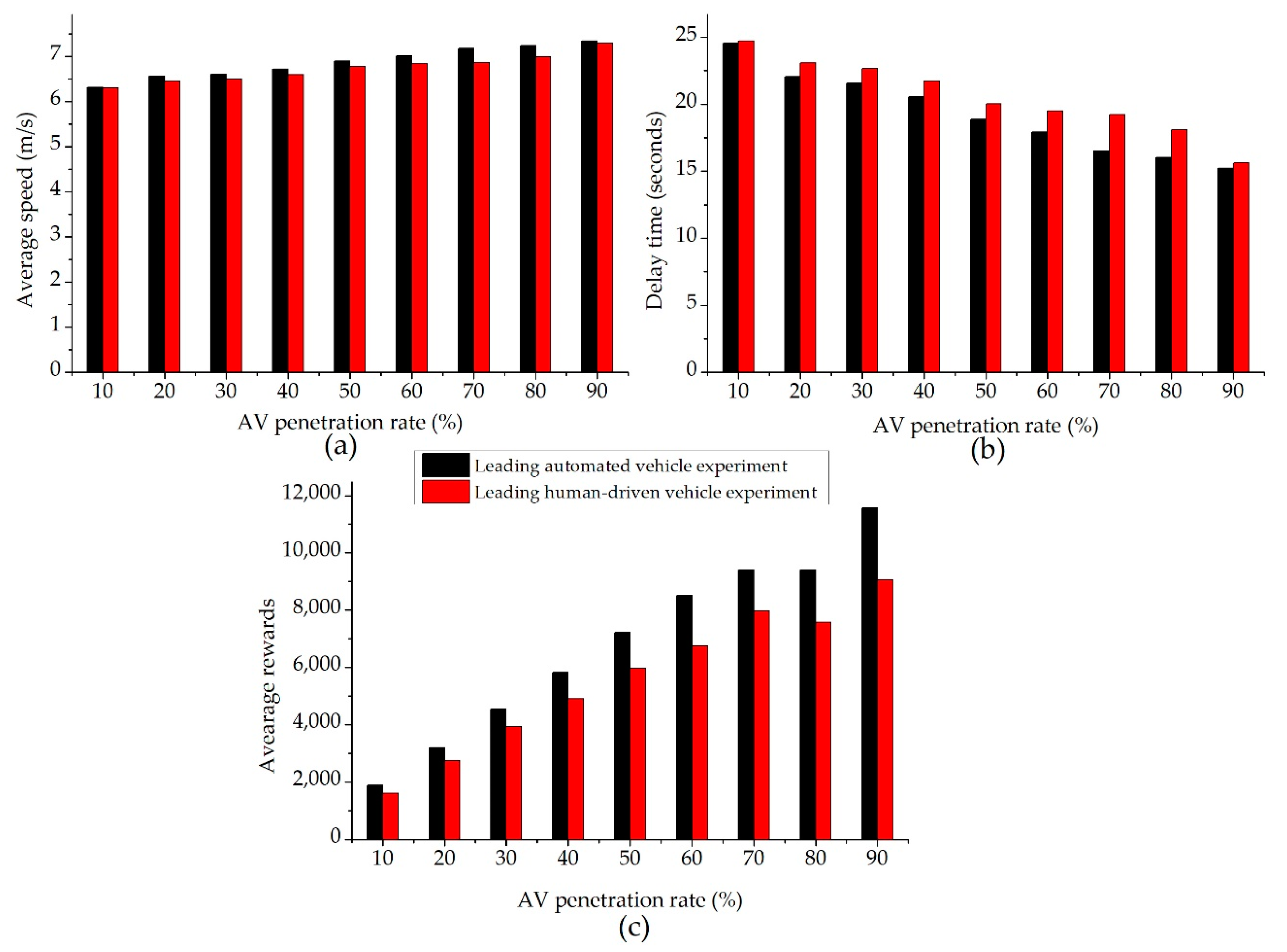
• An enhanced hybrid deep RL method is presented that uses a PPO algorithm through MLP and RL models in order to consider the effectiveness of the leading autonomous vehicle experiment at a non-signalized intersection based on an AV penetration rate that ranges from 10% to 100% in 10% increments. The leading autonomous vehicle experiment yields a significant improvement when compared with the leading human-driven vehicle and all human-driven vehicle experiments in terms of training policy, mobility, and energy efficiency.
• A set of PPO hyperparameters is proposed in order to explore the effect of the automated extraction feature on policy prediction and to obtain reliable simulation performance at a non-signalized intersection within the real traffic volume.
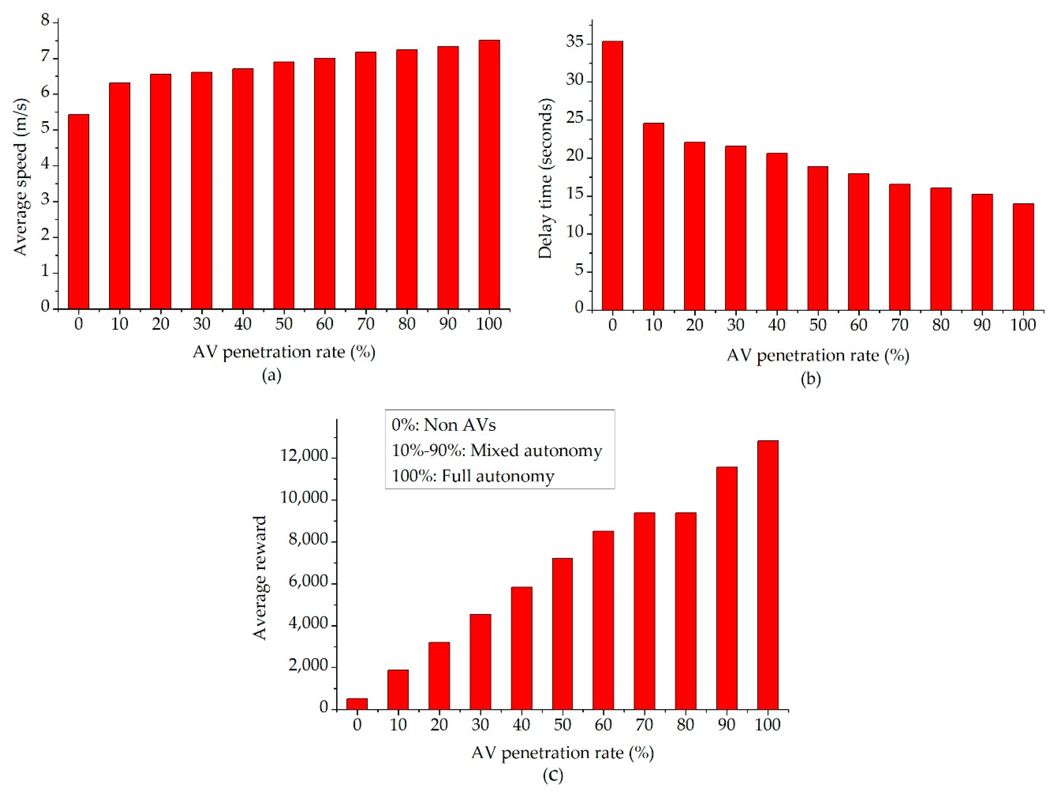
• The demonstration of a significant improvement in traffic perturbations at a non-signalized intersection is based on an AV penetration rate that ranges from 10% to 100% in 10% increments.

The rest of this paper is organized as follows. Section 2 presents the deep RL framework, the longitudinal dynamic models, the policy optimization method, and the proposed model’s architecture. Section 3 describes the simulation experiments and presents the results. Section 4 contains our conclusions.

2. Methods

2.1. Deep Reinforcement Learning (Deep RL)

Reinforcement learning (RL) is a subarea of machine learning and is concerned with how agents interact with an environment and learn to take actions that maximize their cumulative reward. The typical form of the RL algorithm is a Markov decision process (MDP), which is a strong framework used to determine a proper action given a full set of observations [9]. An MDP is a tuple (S, A, P, R, ρ₀, γ, T), where S and A are states and actions of a participant, respectively; P(S’, S, a) defines a probability for transition; R(a, S) defines the reward according to the selected action; ρ₀ defines the initial state distribution; γ defines the discount factor, which ranges from 0 to 1; and T denotes the time horizon. However, automated vehicles maneuver in an uncertain environment that contains inaccuracy, intentions, and sensor noise. To solve this problem, a partially observable MDP (POMDP) was proposed that employs two more components, namely O, which defines the set of observations, and Z, which is an observation function. An objective learning agent in RL optimizes the policy π to maximize their expected cumulative discounted reward over some number of time steps.

A deep neural network (DNN) has the ability to automatically perform feature extraction due to multiple hidden layers of representations. For continuous controllers, artificial neural networks (ANNs) are commonly used methods that employ multiple hidden layers to represent complex functions. In this work, we apply an MLP to generate a set of outputs (policy) from a set of inputs (states and observations). In addition, we apply a PPO based on a gradient descent optimization method to enhance the performance of the DNN. Our proposed deep RL framework, which fuses a MLP and RL, is designed to consider the effectiveness of AVs at a non-signalized intersection. First, the SUMO simulator executes one simulation step. Second, the Flow framework sends information on the SUMO simulator’s state to the RL library. Then, the RL library (RLlib) computes the appropriate action according to SUMO simulator’s state through MLP. The MLP policy is applied to maximize the cumulative reward for the RL algorithm based on the traffic data. Finally, the simulation resets and iterates the RL process. Figure 1 presents the deep reinforcement learning architecture in the context of a non-signalized intersection.

Importantly, a ‘policy’ refers to a blueprint of the communication between perceptions and actions in an environment. In other words, a policy is similar to a controller of a traffic simulation. In this work, the controller is an MLPpolicy with multiple hidden layers. The parameters of the controller are iteratively updated by using the MLPpolicy to maximize the cumulative reward based on the traffic data sampled from the SUMO simulator. The main goal of the agent is to learn how to optimize a stochastic policy as follows.

$${\theta }^{*}:=argma{x}_{\theta }\eta \left({\pi }_0\right)$$

(1)

where$\eta \left({\pi }_0\right)$ is the expected cumulative discounted reward, which is calculated by the discount factor (${\gamma }_i)$ and the reward (r).

$$\eta \left({\pi }_0\right)={{\displaystyle \sum }}_{i=0}^T{\gamma }_i{r}_i$$

(2)

2.2. Longitudinal Dynamic Models

Basic vehicle dynamics can be defined by car-following models, which describe the longitudinal dynamics of a manually operated vehicle based on observations of the vehicle itself and vehicles in front. A standard car-following model is as follows:

$$a_i=f\left(h_i,{\dot{h}}_i,v_i\right)$$

(3)

where a_i is the acceleration of vehicle i, f() is a nonlinear function, and v_i, ${\dot{h}}_i$, and h_i are the velocity, relative velocity, and headway of vehicle i, respectively.

In this work, we apply the IDM, which is a type of ACC system, for the longitudinal control of human-driven vehicles due to its capacity to depict realistic driver behavior [7]. The IDM is a commonly used car-following model. In the IDM’s acceleration command, the speed of a vehicle in a non-signalized intersection environment and the identification (ID) and headway of the leading vehicle can be set to be obtained by the “get” methods. The acceleration of the vehicle is calculated as follows.

$$a_{IDM}=a\left[1-{\left(\frac{v}{v_0}\right)}^{\delta }-{\left(\frac{s^{*}\left(v,\Delta v\right)}{s}\right)}^2\right]$$

(4)

where a_IDM is the acceleration of the vehicle, v₀ is the desired speed, $\delta$ is an acceleration exponent, s is the vehicle’s headway (the distance to the vehicle ahead), and $s^{*}\left(v,\Delta v\right)$ indicates the desired headway, which is expressed by:

$$s^{*}\left(v,\Delta v\right){=s}_0+\mathit{max}\left(0,\mathit{vT}+\frac{v\Delta v}{2\sqrt{\mathit{ab}}}\right)$$

(5)

where S₀ denotes the minimum gap, $T\mathrm{denotes}a\mathrm{time}\mathrm{gap},\Delta v$ denotes the velocity difference compared with the lead vehicle (current velocity–lead velocity), a denotes an acceleration term, and b denotes comfortable deceleration.

The typical parameters of an IDM controller for city traffic are represented in

Table 1. Typical parameters of an intelligent driver model (IDM) controller for city traffic.

Parameters	Value
Desired speed (m/s)	15
Time gap (s)	1.0
Minimum gap (m)	2.0
Acceleration exponent	4.0
Acceleration (m/s2)	1.0
Comfortable acceleration (m/s2)	1.5

based on [41].

2.3. Policy Optimization

Policy gradient methods attempt to compute an estimator of a parameterized policy function using a gradient descent algorithm rather than an action-value or a state-value function. Thus, they avoid the convergence problems that occur with estimation functions due to non-linear approximation and partial observation. We applied the MLP policy to optimize the control policy directly in the simulation of the non-signalized intersection. The policy gradient laws, which are based on the expectation over the probabilities of the policy actions ($\log {\pi }_{\theta }$) and an estimate of the advantage function at time step t (${\widehat{A}}_t$), are expressed as follows.

$$\widehat{g}= {\widehat{E}}_t\left[{\nabla }_{\theta }\log {\pi }_{\theta }\left(a_t|s_t\right){\widehat{A}}_t\right]$$

(6)

where${\widehat{E}}_t[.]$ is the expectation operator over a finite batch of samples, ${\pi }_{\theta }$ indicates a stochastic policy, ${\widehat{A}}_t$ is defined by the discounted sum of rewards and a baseline estimate, and a_t and s_t express the action and state at time step t, respectively.

PPO, which was proposed by Schulman et al. [26], is a simple TRPO that is provided by the RLlib library. In other words, PPO’s objective is the same as that of TRPO, which uses a trust region constraint to force the policy update to ensure that the new policy is not too far away from the old policy. There are two types of PPO: adaptive Kullback–Leibler (KL) penalty and clipped objective. The PPO generates policy updates by adopting a surrogate loss function. This process avoids a reduction in performance during the training process. The surrogate object (J^CPI) is described as follows.

$$J^{CPI}\left(\theta \right)={\widehat{E}}_t\left[\frac{{\pi }_{\theta }\left(a_t|s_t\right)}{{\pi }_{{\theta }_{old}}\left(a_t|s_t\right)}{\widehat{A}}_t\right]={\widehat{E}}_t\left[r_t\left(\theta \right){\widehat{A}}_t\right]$$

(7)

where ${\pi }_{{\theta }_{old}}$indicates a policy parameter before update, ${\pi }_{\theta }$indicates a policy parameter after update, and $r_t\left(\theta \right)$ indicates the probability ratio.

For continuous actions, the PPO’s policy output is a parameter of the Gaussian distribution for each action. The policy then generates a continuous output based on these distributions. In this work, PPO with an adaptive KL penalty is used to optimize the KL-penalized objective by using minibatch stochastic gradient descent (SGD) as follows.

$$\underset{\theta }{\mathrm{maximize}}{\widehat{E}}_t\left[r_t\left(\theta \right){\widehat{A}}_t\right]-\beta {\widehat{E}}_t\left[KL\left[{\pi }_{{\theta }_{old}}\left(a_t|s_t\right),{\pi }_{\theta }\left(a_t|s_t\right)\right]\right]$$

(8)

$$\mathrm{Subject}\mathrm{to} {\widehat{E}}_t\left[KL\left[{\pi }_{{\theta }_{old}}\left(a_t|s_t\right),{\pi }_{\theta }\left(a_t|s_t\right)\right]\right]\le \delta$$

(9)

where$\beta$ is the weight control coefficient that is updated after every policy update. If the current KL divergence is greater than the target KL divergence, we increase β. Similarly, if the current KL divergence is less than the target KL divergence, we decrease β.

In the PPO algorithm, first, the current policy interacts with the environment to generate the episode sequences. Next, the advantage function is estimated using the baseline estimate for the state value. Finally, we collect all experiences and execute the gradient descent algorithm over the policy network. The complete PPO with an adaptive KL penalty algorithm is presented in pseudocode in Algorithm 1, shown below [42]:

Algorithm 1 PPO with an Adaptive KL Penalty Algorithm

1: Initial policy parameters θ0, weight control β0, target KL-divergence δtag 2: For k = 0, 1, 2…do 3: Gather set of trajectories on policy ${\pi }_k=\pi \left({\theta }_k\right)$ 4: Optimize the KL penalized using minibatch SGD $$J^{KLPEN}\left(\theta \right)={\widehat{E}}_t\left[r_t\left(\theta \right){\widehat{A}}_t\right]-\beta {\widehat{E}}_t\left[KL\left[{\pi }_{{\theta }_{old}}\left(a_t|s_t\right),{\pi }_{\theta }\left(a_t|s_t\right)\right]\right]$$ 5: Compute KL divergence between the new and old policy $$\delta ={\widehat{E}}_t\left[KL\left[{\pi }_{{\theta }_{old}}\left(a_t|s_t\right),{\pi }_{\theta }\left(a_t|s_t\right)\right]\right]$$ 6: If δ > 1.5 δtag then βk+1 = 2βk 7: Else if δ < δtag/1.5 then    βk+1 = βk/2 8: Else pass 9: End if 10: End for

Importantly, the PPO hyperparameters provide a robust approach to enhancing the effectiveness of RL at various tasks. In particular, Gamma (γ) is a discount factor that ranges from 0 to 1 and indicates how important future rewards are to the current state. The hidden layers affect the accuracy and performance. With more hidden layers, the accuracy increases; however, the performance decreases. Lambda (λ) is a smoothing rate that reduces the variance during the training process to ensure that training progresses in a stable manner. The Kullback–Leibler (KL) target is the desired policy change for each iteration.

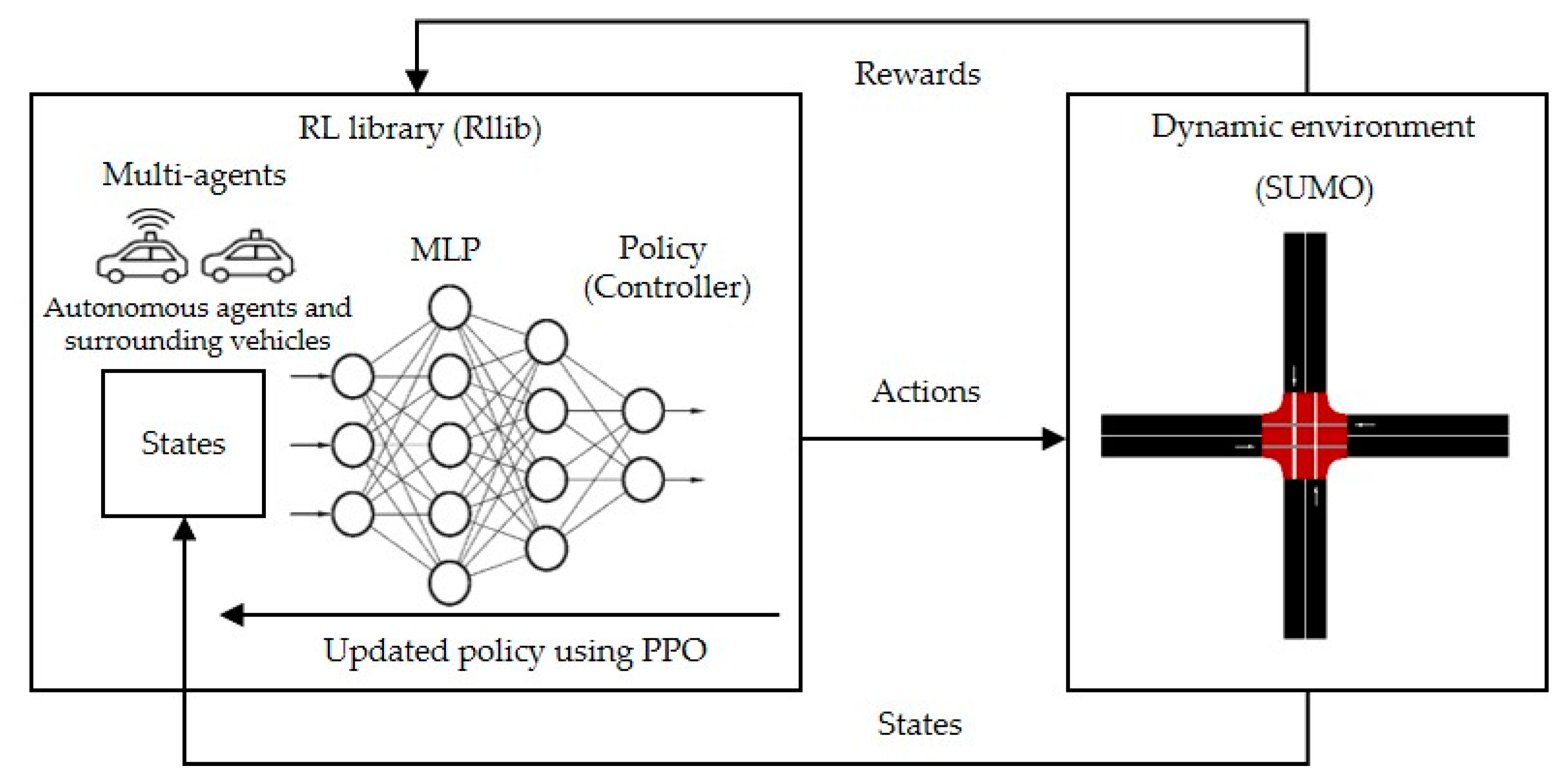
2.4. Proposed Method’s Architecture

In this study, we applied the open-source modular learning framework Flow to connect the RL library (RLlib) to the traffic simulator (SUMO). Flow allows us to simulate varied and complex traffic environments, multiple agents, and multiple algorithms [43]. The implementation is based on SUMO [35], Ray RLlib for RL [44], and the OpenAI gym for the MDP [45]. Our study focuses on an online optimization in a closed-loop setting through deep RL. Figure 2 shows the proposed method’s architecture.

SUMO, developed by the Institute of Transportation Systems at the German Aerospace Center, is an open-source microscopic traffic simulator. SUMO can simulate urban-scale traffic networks along with traffic lights, vehicles, pedestrians, and public transportation. In addition, the TraCI enables SUMO to be connected to Python in order to apply deep RL to the SUMO simulator. A typical SUMO simulator at a non-signalized intersection is shown in Figure 3.

Flow [44], developed by UC Berkeley, provides an interface between deep RL algorithms and custom road networks. Additionally, Flow can analyze and validate a training policy. The advantages of Flow include the ability to easily implement varied road networks in order to enhance controllers for autonomous vehicles through deep RL. In Flow, a custom environment can be used to generate the main subset class, including initialized simulation, observation space, state space, action space, controller, and reward function, for various scenarios.

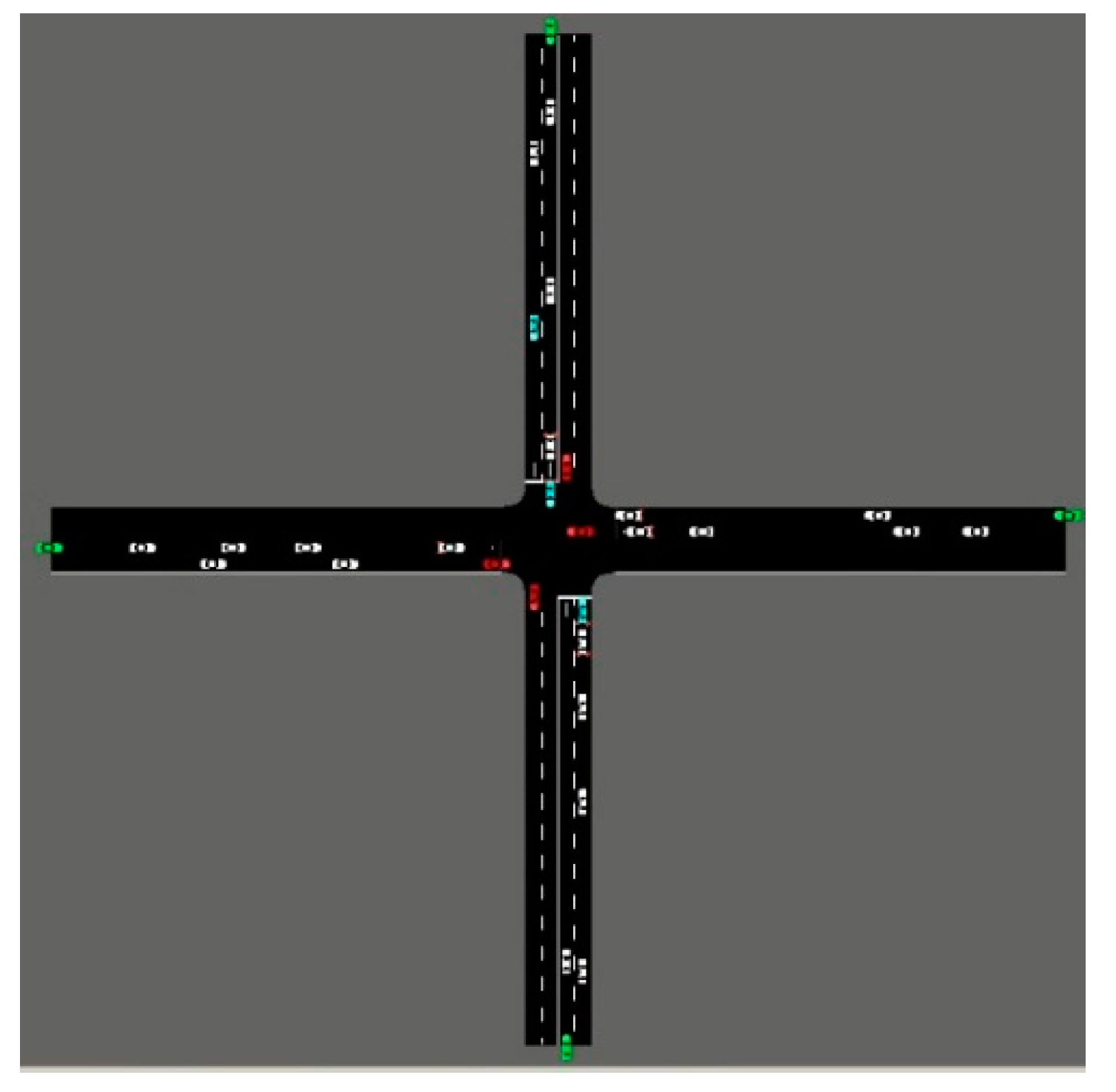
2.4.1. Initialized Simulation

The initialized simulation expresses the initial settings of the simulation environment for the starting episode. In particular, we set up the position, speed, acceleration, starting points, trajectories, and number of vehicles, as well as the parameters of the IDM rules and the deep RL framework. In particular, the trajectories of all vehicles is set in the initialized simulation process by SUMO simulator including specific nodes (the position of points in the network), specific edges (linked the nodes together), and specific routes (the sequence of edges vehicles traverse). Next, the acceleration of human-driven vehicles is controlled by the SUMO simulator and the acceleration of AVs is controlled by Rllib library.

2.4.2. Observation Space

The observation space expresses the number and types of observable features, namely the AV speed (ego vehicle speed), the AV position (ego position), and the speeds and bumper-to-bumper headways of the corresponding preceding and following AVs described in Figure 4. The observable output is fed into the state space to predict the proper policy.

2.4.3. State Space

A state space represents a vector of autonomous agents and surrounding vehicles based on the observation space, including the positions and velocities of AVs, as well as preceding and following AVs. The features within the environments are extracted and fed into the policy using the get_state method. First, we obtain the ID of all vehicles at the non-signalized intersection. Then, the positions and velocities of all vehicles are obtained to generate the state space. Importantly, the current position is based on pre-specified starting point. The state space is defined as follows:

$$S= \left(\begin{array}{c}{x}_0\\ \begin{array}{c}{v}_0\\ \begin{array}{c}{v}_l\\ d_l\end{array}\\ \begin{array}{c}{v}_f\\ d_f\end{array}\end{array}\end{array}\right)$$

(10)

where S is the state of a specific vehicle, x₀ is the corresponding coordinates of the AV, v₀, v_l, and v_f are the corresponding speeds of the AV, the preceding AV, and the following AV, respectively, and d_l and d_f denote the bumper-to-bumper headways of the preceding AV and the following AV, respectively.

2.4.4. Action Space

The action space represents the actions of the autonomous agents in the traffic environment provided by the OpenAI gym. The standard action for an automated vehicle would be an acceleration. In the action space, the bounds of the actions range from maximum deceleration to maximum acceleration. Then, the apply_RL_actions function is applied to transform a specific command into an actual action in the SUMO simulator. First, we identify all AVs at the non-signalized intersection. Then, the action commands are converted into accelerations using the base environment method.

2.4.5. Controller

The controller controls the behaviors of the actors, including human-driven vehicles and AVs. A single controller can be applied to multiple actors using shared control. In this work, the human-driven vehicles are controlled by the Flow framework, and the automated vehicles are controlled by the RLlib library.

2.4.6. Reward Function

In order to reduce the traffic congestion, we need to optimize the average speed of the network thanks to reducing delay time, queue lengths. Therefore, the average speed has become a promising metric to train deep RL policy in the real world. The reward function defines the way in which an autonomous agent will attempt to optimize a policy. In this work, the goal of an RL agent is to obtain a high average speed while punishing collisions between vehicles at a non-signalized intersection. In this study, the L2 norm was used to estimate the positive distance given the speed of a vehicle at a non-signalized intersection based on the target speed (the desired speed of all vehicles at a non-signalized intersection). In particular, we applied the get-speed method to obtain the current speed of all vehicles at the non-signalized intersection and then return the average speed as the reward. The reward function is expressed as follows [32]:

$$r_t:=max(\Vert v_{des}·{𝕝}^k{\Vert }_2-\Vert v_{des}-v{\Vert }_2,0)/\Vert v_{des}·{𝕝}^k{\Vert }_2$$

(11)

where v_des denotes an arbitrary desired speed and v ϵ R^k denotes the speeds of all vehicles at a non-signalized intersection.

2.4.7. Termination

The termination of a rollout is based on the training iteration and collisions as follows: (1) the training iteration is complete; (2) a collision between two vehicles occurred.

3. Experimental Results and Analysis

3.1. Hyperparameter Setting and Evaluation Metrics

The PPO with an adaptive KL penalty algorithm controls the distance between the updated policy and the old policy in order to avoid noise during a gradient update. Hyperparameter tuning was used to select the proper variables for the training process. Hence, PPO hyperparameter initializations improve the effectiveness of RL at various tasks. In this study, we propose the set of PPO hyperparameters for mixed-autonomy traffic at a non-signalized intersection shown in

Table 2. Proximal policy optimization (PPO) hyperparameters for mixed-autonomy traffic at a non-signalized intersection.

Parameters	Value
Number of training iterations	200
Time horizon per training iteration	6000
Gamma	0.99
Hidden layers	256 × 256 × 256
Lamda	0.95
Kullback–Leibler (KL) target	0.01
Number of SGD iterations	10

. The time horizon per training iteration is calculated by multiplication between the time horizon of a single rollout and the number of rollouts per training iteration. The time horizon of a single rollout is 600 and the number of rollouts per training iteration is 10. Therefore, the time horizon per training iteration is 6000. The “256 × 256 × 256” means that we set up 3 hidden layers, and each layer has 256 neurons at all. In addition, based on our experiment, the agent performs well at the number of training iteration of 200.

The training policy’s performance was verified by the maximum reward curve over 200 iterations. A flattening of the curve indicates that the training policy has completely converged. Furthermore, the simulation performance was evaluated by measures of effectiveness (MOE), which are designed to analyze traffic operations. Such an evaluation can help to predict and address traffic issues. In this study, we adopted the following MOE to evaluate the simulation’s performance:

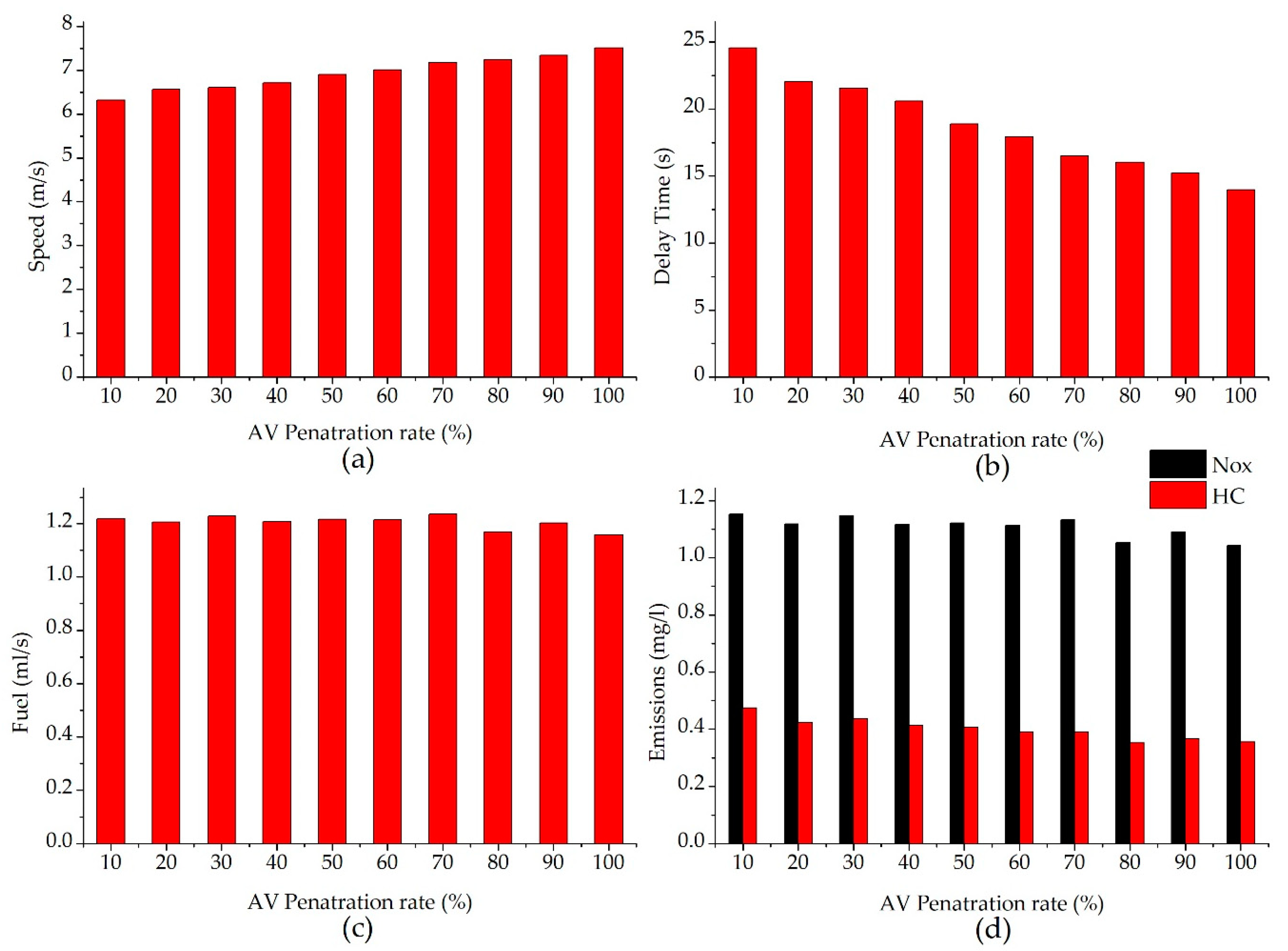
• Mean speed: the average speed of all vehicles at a non-signalized intersection.
• Delay time: the time difference between real and free-flow travel times of all vehicles.
• Fuel consumption: the average fuel consumption value of all vehicles.
• Emissions: the average emission values of all vehicles, including nitrogen oxide (NOx) and hydrocarbons (HC).

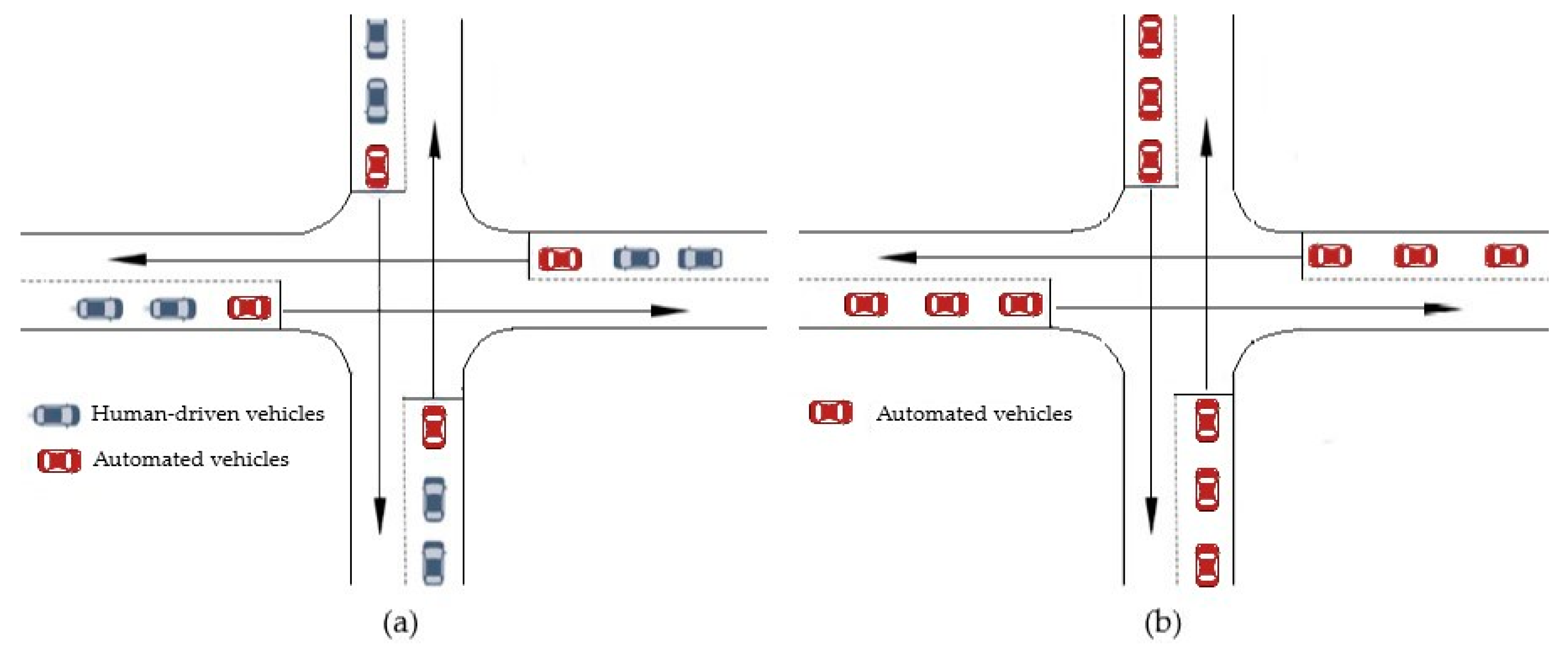
3.2. Experimental Scenarios

In this study, vehicles that crossed the non-signalized intersection followed a right-of-way rule supplied by the SUMO simulator. The objective of the right-of-way rule is to enforce traffic rules and also avoid traffic collisions. Moreover, we observed the positions of all vehicles and converted the environment from a POMDP to an MDP. Importantly, autonomous agents learned to optimize a certain reward over the rollouts using the RLlib library. Our simulation uses RL agents to represent a human-driven fleet and an entire traffic flow in mixed-autonomy traffic. The RL agents receive the updated state and bring about a new state in time steps of 0.1 s. For human-driven vehicles, acceleration behaviors are controlled by the IDM model. Furthermore, continuous routing is applied to maintain the vehicles within the network.

We executed the simulation experiments with time steps of 0.1 s, a lane width of 3.2 m, two lanes in each direction, a lane length in each direction of 420 m, a maximum acceleration of 3 m/s², a minimum acceleration of –3 m/s², a maximum speed of 12 m/s, a horizon of 600, and 200 iterations for the training process. We set an inflow of 1000 vehicles per hour in each direction. The range of the non-signalized intersection was between 200 m and 220 m. In the field, many different scenarios must be simulated. However, in this study, we limited our focus to the effectiveness of the leading autonomous vehicle at a non-signalized intersection. Platooning vehicles approach a non-signalized intersection and drive straight ahead following four different directions. In addition, we also present the results for AV penetration rates ranging from 1% to 100% in 10% increments. Importantly, we ignored lane changing and turning left for all vehicles at the non-signalized intersection. Figure 5 shows the leading autonomous vehicle experiment at the non-signalized intersection.

To demonstrate the superiority of the leading autonomous vehicle experiment, we compared the leading autonomous vehicle experiment with other experiments, including the leading human-driven vehicle experiment and the all human-driven vehicle experiment. Figure 6 shows a comparison of the experiments at a non-signalized intersection.

3.3. Experimental Results and Analysis

3.3.1. Training Policy’s Performance

The RL training performance through the AV penetration rate was used to evaluate the learning performance. Figure 7 shows the average reward curve over 200 iterations based on the AV penetration rates. The flattening of the curve in all circumstances indicates that the training policy had almost converged. Moreover, the average reward increased as the AV penetration rate at the non-signalized intersection increased, except for the 50% AV penetration rate. Full-autonomy traffic outperformed the other AV penetration rates; it produced the highest average reward and significant flattening of the curve. In particular, full-autonomy traffic yielded an improvement of 6.8 times compared with the 10% AV penetration rate. Therefore, full-autonomy traffic outperformed the other AV penetration rates in all circumstances. The effectiveness of the leading autonomous vehicle experiment at the non-signalized intersection became more obvious as the AV penetration rate increased.

3.3.2. Effect of the Leading Automated Vehicle on the Smoothing Velocity

We considered the effect of the leading automated vehicle on the smoothing velocity. Figure 8 shows the spatio-temporal dynamics through the AV penetration rate at the non-signalized intersection. The points are color-coded based on the velocity. The points closer to the top denote smooth traffic. In contrast, the points closer to the bottom denote congested traffic. For the lower AV penetration rates, perturbations occurred due to stop-and-go waves of human-driven vehicle behavior, reducing the velocity in the non-signalized intersection area (ranging from 200 m to 220 m). As can be seen in Figure 8, almost all of the points are close to the bottom in the non-signalized intersection area with the lower AV penetration rates. This is because human-driven vehicles simultaneously approach the non-signalized intersection area and slow down according to the right-of-way rule. At the higher AV penetration rates, the points are close to the top, with the AVs slowing down in a shorter time, thereby producing fewer and shorter stop-and-go waves in the non-signalized intersection area. Full-autonomy traffic achieved the highest smoothing velocity of all AV penetration rates. Thus, the traffic congestion was partially cleared, and traffic flow became smoother as the AV penetration rate increased.

3.3.3. Effect of the Leading Automated Vehicle on Mobility and Energy Efficiency

Figure 9 shows the MOE evaluation in terms of average speed, delay time, fuel consumption, and emissions based on the AV penetration rates. The results of the MOE evaluation indicate that the simulation became more effective as the AV penetration rate increased. Regarding mobility, the average speed gradually increased and the delay time gradually decreased as the AV penetration rate increased. As can be seen in Figure 9a,b, full-autonomy traffic achieved an improvement in average speed of 1.19 times and an improvement in delay time of 1.76 times compared with the 10% AV penetration rate. The energy efficiency, fuel consumption, and emissions slightly decreased as the AV penetration rate increased. As shown in Figure 9c,d, full-autonomy traffic achieved an improvement in fuel consumption of 1.05 times and an improvement in emissions of 1.22 times compared with the 10% AV penetration rate. Thus, leading autonomous vehicles are more effective in terms of mobility and energy efficiency when the AV penetration rate increases.

3.3.4. Performance Comparison

To verify the superiority of the leading autonomous vehicle experiment (the proposed experiment), we compared it with other experiments, including an all human-driven vehicle experiment and a leading human-driven vehicle experiment. The comparison between the proposed experiment and the all human-driven vehicle experiment is shown in Figure 10. Regarding mobility, the proposed experiment achieved a higher average speed and a lower delay time compared with the all human-driven vehicle experiment. As seen in Figure 10a,b, the 10% AV penetration rate achieved an improvement in average speed of 1.16 times and an improvement in delay time of 1.44 times compared with all human-driven vehicle experiment. Furthermore, full-autonomy traffic achieved an improvement in average speed of 1.38 times and an improvement in delay time of 2.55 times compared with the all human-driven vehicle experiment. In terms of energy efficiency, the proposed experiment achieved lower fuel consumption and emissions compared with the all human-driven vehicle experiment. As shown in Figure 10c, the 10% AV penetration rate achieved an improvement in average reward of 3.63 times compared with the all human-driven vehicle experiment. In addition, full-autonomy traffic achieved an improvement in average reward of 24.77 times compared with the all human-driven vehicle experiment. Hence, the proposed experiment outperformed the all human-driven vehicle experiment in terms of both mobility and energy efficiency.

The comparison between the proposed experiment and the leading human-driven vehicle experiment is shown in Figure 11. Regarding mobility, the proposed experiment achieved a higher average speed and a lower delay time compared with the leading human-driven vehicle experiment. As seen in Figure 11a,b, the proposed experiment achieved an improvement in average speed of 1.02 times and an improvement in delay time of 1.06 times compared with the leading human-driven vehicle experiment. In terms of energy efficiency, the proposed experiment achieved lower fuel consumption and emissions compared with the leading human-driven vehicle experiment. As shown in Figure 11c, the proposed experiment achieved an improvement in average reward of 1.22 times compared with the leading human-driven vehicle experiment. Hence, the proposed experiment outperformed the leading human-driven vehicle experiment in terms of both mobility and energy efficiency.

4. Discussion and Conclusions

In this study, we demonstrated that leading autonomous vehicles become more effective in terms of training policy, mobility, and energy efficiency as their AV penetration rates increase. The traffic congestion was partially cleared, and the traffic flow became smoother as the AV penetration rate increased. Full-autonomy traffic was shown to outperform all other AV penetration rates. In particular, full-autonomy traffic improved the average speed and delay time by 1.38 times and 2.55 times, respectively, compared with all human-driven vehicle experiment. The leading autonomous vehicle experiment was shown to outperform both the all human-driven vehicle experiment and the leading human-driven vehicle experiment.

In summary, the leading autonomous vehicle experiment, which uses a set of PPO hyperparameters and deep RL, performed better than the leading human-driven vehicle experiment and the all human-driven vehicle experiment. The main contributions of this work are the proposed set of PPO hyperparameters and the deep RL framework, which together resulted in a reliable simulation of mixed-autonomy traffic at a non-signalized intersection based on the AV penetration rate. The proposed method provides more positive effects when the AV penetration rate increases. Additionally, researchers could adopt the leading autonomous vehicle experiment to dissipate stop-and-go waves. In our future work, we will consider the efficiency of multiple autonomous vehicles for the network with multi-intersections by developing more advanced deep machine learning algorithms.

References

1. National Highway Traffic Safety Administration. Traffic Safety Facts 2015: A Compilation of Motor Vehicle Crash Data from the Fatality Analysis Reporting System and the General Estimates System. The Fact Sheets and Annual Traffic Safety Facts Reports, USA. 2017. Available online: https://crashstats.nhtsa.dot.gov/Api/Public/ViewPublication/812384 (accessed on 26 April 2017).
2. Wadud, Z.; MacKenzie, D.; Leiby, P.N. Help or hindrance? The travel, energy and carbon impacts of highly automated vehicles. Transp. Res. Part A Policy Pract. 2016, 86, 1–18. [Google Scholar] [CrossRef] [Green Version]
3. Fagnant, D.; Kockelman, K. Preparing a nation for automated vehicles: Opportunities, barriers and policy recommendations. Transp. Res. Part A Policy Pract. 2015, 77, 167–181. [Google Scholar] [CrossRef]
4. Rajamani, R.; Zhu, C. Semi-autonomous adaptive cruise control systems. IEEE Trans. Veh. Technol. 2002, 51, 1186–1192. [Google Scholar] [CrossRef]
5. Davis, L. Effect of adaptive cruise control systems on mixed traffic flow near an on-ramp. Phys. A Stat. Mech. Appl. 2007, 379, 274–290. [Google Scholar] [CrossRef] [Green Version]
6. Milanes, V.; Shladover, S.E. Modeling cooperative and autonomous adaptive cruise control dynamic responses using experimental data. Transp. Res. Part C Emerg. Technol. 2014, 48, 285–300. [Google Scholar] [CrossRef] [Green Version]
7. Treiber, M.; Hennecke, A.; Helbing, D. Congested traffic states in empirical observations and microscopic simulations. Phys. Rev. E 2000, 62, 1805–1824. [Google Scholar] [CrossRef] [Green Version]
8. Yang, L.; Zhang, X.; Gong, J.; Liu, J. The Research of Car-Following Model Based on Real-Time Maximum Deceleration. Math. Probl. Eng. 2015, 2015, 1–9. [Google Scholar] [CrossRef] [Green Version]
9. Bellman, R. A Markovian Decision Process. J. Math. Mech. 1957, 6, 679–684. [Google Scholar] [CrossRef]
10. Howard, R.A. Dynamic Programming and Markov Processes; The M.I.T. Press: Cambridge, UK, 1960. [Google Scholar]
11. Sutton, R.; Barto, A. Reinforcement Learning: An Introduction. IEEE Trans. Neural Netw. 1998, 9, 1054. [Google Scholar] [CrossRef]
12. Mnih, V.; Kavukcuoglu, K.; Silver, D.; Graves, A.; Antonoglou, I.; Wierstra, D.; Riedmiller, M. Playing atari with deep reinforcement learning. arXiv 2013, arXiv:1312.5602. [Google Scholar]
13. Silver, D.; Huang, A.; Maddison, C.J.; Guez, A.; Sifre, L.; Driessche, G.V.D.; Schrittwieser, J.; Antonoglou, I.; Panneershelvam, V.; Lanctot, M.; et al. Mastering the game of Go with deep neural networks and tree search. Nature 2016, 529, 484–489. [Google Scholar] [CrossRef] [PubMed]
14. Duan, Y.; Chen, X.; Houthooft, R.; Schulman, J.; Abbeel, P. Benchmarking deep reinforcement learning for continuous control. arXiv 2016, arXiv:1604.06778. [Google Scholar]
15. Bellemare, M.G.; Naddaf, Y.; Veness, J.; Bowling, M. The Arcade Learning Environment: An Evaluation Platform for General Agents. J. Artif. Intell. Res. 2013, 47, 253–279. [Google Scholar] [CrossRef]
16. Todorov, E.; Erez, T.; Tassa, Y. MuJoCo: A Physics Engine for Model-Based Control. In Proceedings of the 2012 IEEE/RSJ International Conference on Intelligent Robots and Systems; Institute of Electrical and Electronics Engineers (IEEE): Vilamoura, Portugal, 7–12 October 2012; pp. 5026–5033. [Google Scholar]
17. Levine, S.; Finn, C.; Darrell, T.; Abbeel, P. End-to-end training of deep visuomotor policies. J. Mach. Learn. Res. 2016, 17, 1–40. [Google Scholar]
18. Tan, K.L.; Poddar, S.; Sarkar, S.; Sharma, A. Deep Reinforcement Learning for Adaptive Traffic Signal Control. In Proceedings of the Volume 3, Rapid Fire Interactive Presentations: Advances in Control Systems; Advances in Robotics and Mechatronics; Automotive and Transportation Systems; Motion Planning and Trajectory Tracking; Soft Mechatronic Actuators and Sensors; Unmanned Ground and Aerial Vehicles; ASME International: Park City, UT, USA, 9–11 October 2019. [Google Scholar]
19. Gu, J.; Fang, Y.; Sheng, Z.; Wen, P. Double Deep Q-Network with a Dual-Agent for Traffic Signal Control. Appl. Sci. 2020, 10, 1622. [Google Scholar] [CrossRef] [Green Version]
20. Gregurić, M.; Vujić, M.; Alexopoulos, C.; Miletić, M. Application of Deep Reinforcement Learning in Traffic Signal Control: An Overview and Impact of Open Traffic Data. Appl. Sci. 2020, 10, 4011. [Google Scholar] [CrossRef]
21. Tan, T.; Bao, F.; Deng, Y.; Jin, A.; Dai, Q.; Wang, J. Cooperative Deep Reinforcement Learning for Large-Scale Traffic Grid Signal Control. IEEE Trans. Cybern. 2019, 50, 2687–2700. [Google Scholar] [CrossRef]
22. Bakker, B.; Whiteson, S.; Kester, L.; Groen, F. Traffic Light Control by Multiagent Reinforcement Learning Systems. ITIL 2010, 281, 475–510. [Google Scholar] [CrossRef]
23. Mnih, V.; Kavukcuoglu, K.; Silver, D.; Rusu, A.A.; Veness, J.; Bellemare, M.G.; Graves, A.; Riedmiller, M.; Fidjeland, A.K.; Ostrovski, G.; et al. Human-level control through deep reinforcement learning. Nat. 2015, 518, 529–533. [Google Scholar] [CrossRef]
24. Mnih, V.; Badia, A.P.; Mirza, M.; Graves, A.; Lillicrap, T.P.; Harley, T.; Silver, D.; Kavukcuoglu, K. Asynchronous methods for deep reinforcement learning. arXiv 2016, arXiv:1602.01783. [Google Scholar]
25. Schulman, J.; Levine, S.; Moritz, P.; Jordan, M.I.; Abbeel, P. Trust region policy optimization. arXiv 2015, arXiv:1502.05477. [Google Scholar]
26. Schulman, J.; Wolski, F.; Dhariwal, P.; Radford, A.; Klimov, O. Proximal Policy Optimization Algorithms. arXiv 2017, arXiv:1707.06347. [Google Scholar]
27. Ye, F.; Cheng, X.; Wang, P.; Chan, C.-Y. Automated Lane Change Strategy using Proximal Policy Optimization-based Deep Reinforcement Learning. arXiv 2020, arXiv:2002.02667. [Google Scholar]
28. Wei, H.; Liu, X.; Mashayekhy, L.; Decker, K. Mixed-Autonomy Traffic Control with Proximal Policy Optimization. In Proceedings of the 2019 IEEE Vehicular Networking Conference (VNC); Institute of Electrical and Electronics Engineers (IEEE): Los Angeles, CA, USA, 4–6 December 2019; pp. 1–8. [Google Scholar]
29. Pomerleau, D.A. An autonomous land vehicle in a neural network. Adv. Neural Inf. Process. Syst. 1988, 1. [Google Scholar]
30. Wymann, B.; Espi’e, E.; Guionneau, C.; Dimitrakakis, C.; Coulom, R.; Sumner, A. TORCS, the Open Racing Car Simulator, v1.3.5. Available online: http://www.torcs.org (accessed on 1 January 2013).
31. Dosovitskiy, A.; Ros, G.; Codevilla, F.; Lopez, A.; Koltun, V. CARLA: An Open Urban Driving Simulator. arXiv 2017, arXiv:1711.03938. [Google Scholar]
32. Behrisch, M.; Bieker, L.; Erdmann, J.; Krajzewicz, D. SUMO—Simulation of Urban MObility: An Overview. In Proceedings of the Third International Conference on Advances in System Simulation, Barcelona, Spain, 23–28 October 2011. [Google Scholar]
33. Krajzewicz, D.; Hertkorn, G.; Feld, C.; Wagner, P. SUMO (Simulation of Urban MObility): An open-source traffic simulation. In Proceedings of the 4th Middle East Symposium on Simulation and Modelling, Dubai, UAE, 2–4 September 2002; pp. 183–187. [Google Scholar]
34. Krajzewicz, D.; Erdmann, J.; Behrisch, M.; Bieker, L. Recent development and applications of sumo-simulation of urban mobility. Int. J. Adv. Syst. Meas. 2012, 5, 128–138. [Google Scholar]
35. Wegener, A.; Piórkowski, M.; Raya, M.; Hellbrück, H.; Fischer, S.; Hubaux, J. TraCI: An Interface for Coupling Road Traffic and Network Simulators. In Proceedings of the 11th Communications and Networking Simulation Symposium, New York, NY, USA, 14–17 April 2008. [Google Scholar]
36. Wu, C.; Parvate, K.; Kheterpal, N.; Dickstein, L.; Mehta, A.; Vinitsky, E.; Bayen, A.M. Framework for Control and Deep Reinforcement Learning in Traffic. In Proceedings of the 2017 IEEE 20th International Conference on Intelligent Transportation Systems (ITSC); Institute of Electrical and Electronics Engineers (IEEE): Yokohama, Japan, 2017; pp. 1–8. [Google Scholar]
37. Vinitsky, E.; Kreidieh, A.; Le Flem, L.; Kheterpal, N.; Jang, K.; Wu, F.; Liaw, R.; Liang, E.; Bayen, A.M. Benchmarks for Reinforcement Learning in Mixed-Autonomy Traffic. In Proceedings of the Conference on Robot Learning, Zürich, Switzerland, 29–31 October 2018. [Google Scholar]
38. Wu, C.; Kreidieh, A.; Parvate, K.; Vinitsky, E.; Bayen, A.M. Flow: Architecture and Benchmarking for Reinforcement Learning in Traffic Control. arXiv 2017, arXiv:1710.05465. [Google Scholar]
39. Wu, C.; Kreidieh, A.; Vinitsky, E.; Bayen, A.M. Emergent behaviors in mixed-autonomy traffic. In Proceedings of the 1st Annual Conference on Robot Learning, Mountain View, CA, USA, 13–15 November 2017; Volume 78, pp. 398–407. [Google Scholar]
40. Kreidieh, A.R.; Wu, C.; Bayen, A.M. Dissipating Stop-and-Go Waves in Closed and Open Networks Via Deep Reinforcement Learning. In Proceedings of the 2018 21st International Conference on Intelligent Transportation Systems (ITSC); Institute of Electrical and Electronics Engineers (IEEE): Maui, Hawaii, USA, 2018; pp. 1475–1480. [Google Scholar]
41. Treiber, M.; Kesting, A. Traffic Flow Dynamics. Traffic Flow Dynamics: Data, Models and Simulation; Springer Berlin Heidelberg: Berlin, Heidelberg, 2013. [Google Scholar] [CrossRef]
42. Graesser, L.; Keng, W.L. Foundations of Deep Reinforcement Learning: Theory and Practice in Python; Addison-Wesley Professional: Boston, MA, USA, 2019; Chapter 7. [Google Scholar]
43. Wu, C.; Kreidieh, A.; Parvate, K.; Vinitsky, E.; Bayen, A.M. Flow: A Modular Learning Framework for Autonomy in Traffic. arXiv 2017, arXiv:1710.05465v2. [Google Scholar]
44. Liang, E.; Liaw, R.; Nishihara, R.; Moritz, P.; Fox, R.; Gonzalez, J.; Goldberg, K.; Stoica, I. Ray RLlib: A composable and scalable reinforcement learning library. arXiv 2017, arXiv:1712.09381. [Google Scholar]
45. Brockman, G.; Cheung, V.; Pettersson, L.; Schneider, J.; Schulman, J.; Tang, J.; Zaremba, W. OpenAI Gym. arXiv 2016, arXiv:1606.01540. [Google Scholar]
Figure 1. The deep reinforcement learning architecture in the context of a non-signalized intersection.
Applsci 10 05722 g001
Figure 2. The proposed method’s architecture.
Applsci 10 05722 g002
Figure 3. A typical A simulation of urban mobility (SUMO) at a non-signalized intersection.
Applsci 10 05722 g003
Figure 4. A typical observation space.
Applsci 10 05722 g004
Figure 5. Leading autonomous vehicle experiments at a non-signalized intersection: (a) mixed-autonomy traffic with autonomous vehicle (AV) penetration rates ranging from 10% to 90% in 10% increments; (b) full-autonomy traffic with a 100% AV penetration rate.
Applsci 10 05722 g005
Figure 6. Comparison of experiments at a non-signalized intersection: (a) the all human-driven vehicle experiment with a 0% AV penetration rate; (b) the leading human-driven vehicle experiment with AV penetration rates ranging from 10% to 90% in 10% increments.
Applsci 10 05722 g006
Figure 7. The average reward curve over the 200 iterations based on the AV penetration rate.
Applsci 10 05722 g007
Figure 8. The spatio-temporal dynamics based on the AV penetration rate.
Applsci 10 05722 g008
Figure 9. The results of the measures of effectiveness (MOE) evaluation based on the AV penetration rate: (a) average speed vs. AV penetration rate; (b) delay time vs. AV penetration rate; (c) fuel consumption vs. AV penetration rate; and (d) emissions vs. AV penetration rate.
Applsci 10 05722 g009
Figure 10. Comparison between the leading autonomous vehicle experiment and the all human-driven vehicle experiment: (a) average reward vs. AV penetration rate; (b) average speed vs. AV penetration rate; and (c) delay time vs. AV penetration rate.
Applsci 10 05722 g010
Figure 11. Comparison between the leading autonomous vehicle experiment and the leading human-driven vehicle experiment: (a) average reward vs. AV penetration rate; (b) average speed vs. AV penetration rate; and (c) delay time vs. AV penetration rate.
Applsci 10 05722 g011