Modeling the Formation of Urea-Water Sprays from an Air-Assisted Nozzle

Abstract

Ammonia preparation from urea-water solutions is a key feature to ensure an effective reduction of nitrogen oxides in selective catalytic reduction (SCR) systems. Thereby, air-assisted nozzles provide fine sprays, which enhance ammonia homogenization. In the present study, a methodology was developed to model the spray formation by means of computational fluid dynamics (CFD) for this type of atomizer. Experimental validation data was generated in an optically accessible hot gas test bench using a shadowgraphy setup providing droplet velocities and size distributions at designated positions inside the duct. An adaption of the turbulence model was performed in order to correct the dispersion of the turbulent gas jet. The spray modeling in the near nozzle region is based on an experimentally determined droplet spectrum in combination with the WAVE breakup model. This methodology was applied due to the fact that the emerging two-phase flow will immediately disintegrate into a fine spray downstream the nozzle exit, which is also known from cavitating diesel nozzles. The suitability of this approach was validated against the radial velocity and droplet size distributions at the first measurement position downstream the nozzle. In addition, the simulation results serve as a basis for the investigation of turbulent dispersion phenomena and evaporation inside the spray.

1. Introduction

Emission legislation is nowadays a crucial factor for the development of internal combustion engines in a wide range of applications. An adherence to the latest thresholds for pollutant emissions requires the use of aftertreatment systems with high conversion rates. Thereby, selective catalytic reduction (SCR) has proven to provide an effective method for cleaning the exhaust gas of diesel engines from nitrogen oxides, with efficiencies higher than 90% [1]. Thus, SCR systems are already state-of-the-art, from small engines for passenger cars up to large engines for the maritime transport [2,3]. The working principle of an SCR system is based on the injection of an aqueous urea solution into the hot exhaust gas. Following the evaporation of the water content, urea undergoes thermo- and hydrolysis reactions and forms the reducing agent ammonia, which reacts with nitrogen oxides to pure nitrogen and water at the catalyst [4].

The high reliability and efficiency of the system require an appropriate preparation of the urea-water spray to ensure fast evaporation and to avoid the formation of deposits from urea. Therefore, depending on the general mixing strategy of the system, an atomization process producing a fine spray with a small initial Sauter mean diameter (SMD) may be favorable. Pressure-driven urea dosing systems usually work with small injection pressures less than 10 bar, which is not sufficient to provide an appropriate atomization. These concepts rather rely on wall wetting and liquid film formation on the hot surfaces of mixing elements that promotes the fast preparation of the aqueous urea solution, as well as the homogeneous distribution of gaseous ammonia in the turbulent flow of the mixing pipe upstream the SCR catalyst [5]. However, increasing the injection pressure as shown by the authors in [6] promotes the atomization process. Air-assisted atomizers, on the other hand, constitute an interesting alternative to achieve a fine spray and high ammonia formation rates without wall interactions. This kind of nozzle is exclusively used in heavy-duty vehicles, as these are often already equipped with compressed air systems [7]. A comparison between pressure-driven and air-assisted systems was conducted by Spiteri et al. [8] by means of optical experiments. They measured a decrease of the SMD from 70 µm for a pressure-driven system to 15 µm for an air-assisted nozzle, which leads to less wall wetting and an improvement of the ammonia distribution. Similar findings were made by Liao et al. [9], who carried out optical investigations of different pressure-driven and air-assisted injection systems. The fine spray generated from the air-assisted nozzle follows the exhaust gas flow and is highly susceptible to its flow conditions, which enables an appropriate prevention of wall wetting and deposit formation.

Numerical flow simulations have nowadays an important role in the development process of aftertreatment systems. In addition to the exhaust gas flow, spray preparation, wall wetting, deposit formation and ammonia distribution are part of numerical models. An overview of the modeling approaches used for SCR systems and the ongoing challenges is given by Lauer in [10]. Many investigations concerning spray preparation can be found in literature. Those studies are, for the most part, focused on the modeling of pressure-driven systems; for example, in [11,12]. Thereby, even advanced methods like large eddy simulation (LES) and volume-of-fluid approaches, which require a high computational effort, are applied to study the breakup of the liquid jet and the formation of initial droplets [13,14]. However, less is reported about the modeling of air-assisted systems in the context of SCR. Chen et al. [15] modeled a twin-fluid atomizer for stationary SCR systems with an external mixing of urea and compressed air. The urea injection was depicted using a blob injection approach assuming an intact liquid core, and the compressed air was introduced by an annular mass flow boundary. Detailed data about the atomization process is not presented due to the focus of this study being on the mixing element. A more detailed investigation of the spray atomization process of air-assisted nozzles was conducted by Naik et al. [16]. In this study, an atomizer with the external mixing of urea and compressed air was investigated by means of phase Doppler anemometry (PDA) measurements and CFD simulations. The authors also used a blob injection approach to initialize the liquid urea-water solution. A good agreement could be achieved for the velocities and the characteristic spray parameters like the SMD and arithmetic diameter.

In the present study, a spray model of an air-assisted atomizer with an internal mixing chamber was generated in a commercial CFD code. Detailed experimental data for the evaluation of the model comprising droplet velocities and droplet sizes at different axial and radial positions was already published by Lieber [17,18] and was provided for the present investigations. The frequently used blob injection approach is not very well-suited for this kind of nozzle, since the liquid and the atomizing air form a complex two-phase flow upstream of the nozzle exit. Therefore, the modeling approach was to extend the computational domain in order to include the outflow channel of the nozzle. This way, defined boundary conditions could be provided for the gas flow. The compressed air was modeled by a gas jet initialized inside this outflow channel. Thereby, modifications of the turbulence model were conducted to adapt the shape of the emerging gas jet. The liquid phase was initialized by a spatially averaged droplet spectrum measured 50 mm downstream the nozzle. The WAVE breakup model, which is quite common for the modeling of breakup processes in the case of diesel injection, was applied to model the atomization of the droplets. Finally, a good agreement with the experimental data could be achieved over a wide range using the presented modeling approach. Particularly, the radial distributions of droplet sizes and velocities could be predicted correctly for different operating conditions, which is important for a correct description of the spray preparation. Further on, the turbulence level inside the jet is discussed due to its influence on the droplet dispersion, as reported by Ström et al. [19]. The findings in the present study contribute to provide and to improve modeling approaches for air-assisted atomizers.

2. Experimental and Numerical Methods

In the scope of an experimental investigation at the Institute of Thermal Turbomachinery of the Karlsruhe Institute of Technology (Karlsruhe, Germany) validation, data was generated that can be used to evaluate evaporating urea-water sprays under realistic thermodynamic and flow conditions. Based on this experimental work, numerical simulations were carried out at the Institute for Powertrains and Automotive Technology (Vienna, Austria) with regard to predicting the spray characteristics of the air-assisted atomizer. In order to derive an appropriate computational methodology for this task, the relevant aspects of the experimental setup will be discussed briefly. Subsequently, the numerical modeling will be elucidated in detail.

2.1. Experimental Setup

A picture of the test rig and the measurement technique is shown in Figure 1a in order to illustrate the experimental setup. The test rig was designed for experimental studies at elevated temperature and pressure conditions covering pre- and post-turbo injection scenarios of the urea-water solution. The atomizer is arranged on the center axis of a pipe flow, which is schematically illustrated in Figure 1b. This generic design was chosen in order to avoid droplet-wall interaction over a long distance downstream of the atomizer. Furthermore, the generic setup provides well-defined boundary conditions, which ensures the applicability of the experimental data for the validation of numerical simulations.

The size and velocity of individual droplets were obtained using microscopic imaging diagnostics, which have been developed to handle the challenging thermodynamic conditions of the hot gas flow around the atomizer [17]. Moreover, a suitable calibration procedure was developed in order to determine the droplet size, with an uncertainty in the range of the pixel resolution of 0.75 µm [18]. This provides the basis for deriving the uncertainty of the velocity determination from the shift of one pixel within the time between two images of 0.5 µs. Hence, the experimental uncertainty of determining the droplet velocity is estimated to be 1.5 m/s.

One merit of this measurement technique is the ability to change the measurement position by simply moving the camera in the direction of its optical axis, while the illumination can stay in a fixed position, as illustrated in Figure 1b. By doing so, detailed correlations of the droplet diameter and velocity were recorded in the proximity of the atomizer [17,18]. These spray characteristics were used to derive the droplet starting conditions for the numerical simulations and to validate the numerical methodology for predicting the spray formation process.

The air-assisted atomizer used in the experiments was manufactured by CALDYN Apparatebau GmbH (Ettlingen, Germany). This atomizer employs the effervescent atomization principle, which involves a two-phase flow upstream of the discharge orifice [20]. In Figure 2, a simplified geometry of the nozzle illustrates the working principle. According to the review on effervescent atomization by Sovani et al. [20], the two main functions of the two-phase flow inside of the atomizer are the lower effective discharge orifice cross section for the liquid phase and the rapidly expanding gas phase as soon as the bubbly flow leaves the nozzle exit. In particular, the rapidly expanding gas enables a fine atomization at relatively low injection pressures in comparison to other methods of atomization.

In the context of exhaust gas aftertreatment systems using SCR technology, a fine atomization is indispensable to ensure a fast and homogeneous conversion of the urea-water solution to ammonia and to avoid the formation of deposits. In addition, the relatively large orifice diameter may be helpful to prevent clogging problems of the atomizer. The decisive advantage of the effervescent atomizer for the experimental setup is a narrow spray angle and, at the same time, a very fine atomization. In combination with the geometry of the configuration, a significant amount of the injected urea-water solution will evaporate before the wall contact of the spray droplets becomes relevant. Hence, it is possible to extract detailed evaporation characteristics of the urea-water spray at different distances downstream of the atomizer, which is discussed in detail in a previous study of Lieber et al. [17]. This experimental data has been employed to evaluate the numerical predictions of the evaporation characteristics in the present study. The main objective is, however, the modeling of the spray formation process of the air-assisted atomizer. Therefore, the comparison of the numerical results with the experimental data will be focused on the spray characteristics in the near nozzle region.

2.2. Computational Method

Numerical simulations of the investigated twin fluid atomizer were carried out using the commercial CFD code AVL FIRE^™ (R2018.1, AVL List GmbH, Graz, Austria). The geometry of the test rig was depicted using the automated meshing procedure FAME^™ Hexa, providing a hexahedral based computational mesh. A spray model was generated by means of a Euler-Lagrange approach to get a deeper insight into the spray formation and propagation. Additionally, the gas jet formed by the escaping compressed air was modeled to provide an appropriate numerical method to predict the behavior of this kind of nozzle. In the following subsections, the modeling of the injection process will be described in detail.

2.2.1. Mesh Generation

The computational mesh of the hot gas test bench contains the inflow section starting downstream of a turbulence grid and has a total length of 1060 mm from inlet to outlet in order to capture all four measurement positions chosen for the experiment. This also provides the opportunity to investigate the experimentally observed evaporation behavior of the urea-water droplets in the hot gas flow. The axial dimension of the mesh requires a local adaption of the cell size to keep the total cell count and the resulting computational effort manageable. Starting from a base cell size of 2°mm in the inflow and outflow area, the cells are step-by-step refined down to 125 µm close to the nozzle in order to ensure an appropriate resolution of the momentum transport of the expanding gas jet and the momentum exchange with the liquid droplets. On the other hand, the cells are sufficiently big compared to the droplet size to comply with the numerical recommendations of the Euler-Lagrange approach. A spray image from the experiment of the near nozzle area is shown in Figure 3a. A plane cut along the center axis of the computational mesh at this near nozzle area is depicted in Figure 3b. Thereby, the refinements are denoted with their corresponding size, and the radial range of the first measurement positions downstream of the atomizer are illustrated.

The outflow channel of the nozzle is depicted by the model to provide defined boundary conditions for the simulation of the gas jet. With a bore diameter of 2 mm and a length of 2 mm, the channel is resolved with around 8200 cells. Using a cell size of 125 µm at the nozzle exit is necessary to capture the high velocity gradients in the radial direction occurring during the expansion of the gas jet. This is of particular importance in the case of the present atomizer, since the gas jet reaches Mach numbers greater than one. The diameter of the nozzle orifice is resolved with 16 cells, which depicts a fine enough resolution. Li et. al. [21] found a resolution of 10 cells appropriate to reduce the grid dependence of the solution of an expanding gas jet, while Abraham et al. [22] recommended at least 8 cells. The mesh is coarsened 25 mm downstream of the nozzle exit to 250 µm, which still provides a fine resolution of the jet. This refinement level covers the first measurement position 50 mm downstream of the atomizer (see Figure 3) and enables an evaluation of the radial velocity profile of the gas jet and the spray characteristics. An overview of all implemented mesh refinements and their dimensions related to the nozzle exit is given in

Table 1. Mesh refinements with dimensions related to the nozzle exit.

Cell Size (mm)	Distance from Nozzle (mm)	Radius (mm)
0.125	25	3
0.25	70	11
0.5	125	15
1	297	35.15

.

2.2.2. Treatment of the Turbulent Gas Jet

The air flow escaping from the twin-fluid atomizer forms a single turbulent gas jet. This gas jet is accelerated to supersonic velocity, due to the under-expanded flow condition in the outflow channel of the nozzle. An under-expanded flow occurs if the pressure ratio of the compressed air in the mixing chamber to the surrounding pressure in the test section exceeds the critical pressure ratio [23]. Before the turbulent gas jet is initialized, the hot air flow in the test rig is precalculated until it achieves convergence. The gas jet is then initialized by means of a mass flow boundary in the outflow channel of the nozzle in the computational domain. The temperature of the gas flow inside of the atomizer has been experimentally determined by means of a thermocouple, which is situated directly upstream of the mixing chamber. On this basis, the temperature of the final mixture of the gas and liquid phase within the mixing chamber is used as an estimate of the initial temperature of the gas jet in the computational domain. In contrast to the initial temperature, no information about the initial turbulence level of the gas jet is available. Hence, a standard turbulence level of 5% is initialized as a rough estimate.

A compressible solver, able to take into account supersonic flows [24], is applied for the calculations. Second-order accuracy differencing schemes are chosen for spatial discretization, and a first-order accuracy scheme is used for temporal discretization. The timestep is set to 1 µs to achieve an appropriate temporal resolution. The turbulent flow is calculated using the Reynolds-averaged Navier-Stokes equations with the k-ε turbulence model. Equations (1)–(5) illustrate the transport equations of turbulent kinetic energy k and turbulent dissipation ε in dependence of the coordinate x, the time t, and the velocity U. The viscosity and the turbulent viscosity are represented by µ and µ_t. S represents the stress tensor in the production term of the turbulence P.

$$\rho \frac{\partial k}{\partial t}+\rho U_j\frac{\partial k}{\partial x_j}=P+G-\epsilon +\frac{\partial }{\partial x_j}\left(\mu +\frac{{\mu }_t}{{\sigma }_k}\frac{\partial k}{\partial x_j}\right)$$

(1)

$$\rho \frac{D\epsilon }{Dt}=\left(C_{\epsilon 1}P+C_{\epsilon 3}G+C_{\epsilon 4}k\frac{\partial U_k}{\partial x_k}-C_{\epsilon 2}\epsilon \right)\frac{\epsilon }{k}+\frac{\partial }{\partial x_j}\left(\frac{{\mu }_t}{{\sigma }_{\epsilon }}\frac{\partial \epsilon }{\partial x_j}\right)$$

(2)

$$P=2{\mu }_{t}S*S-\left(\frac{2}{3}\right)\left[{\mu }_t\left(trS\right)+k\right]\left(trS\right)$$

(3)

$$G=-\frac{{\mu }_t}{\rho {\sigma }_{\rho }}\nabla \rho$$

(4)

$${\mu }_t=C_{\mu }\rho \frac{k^2}{\epsilon }$$

(5)

The model contains eight constants, which are available for calibration. In the present implementation, the standard values listed in

Table 2. Standard values of the parameters of the k-ε model.

Parameter	Standard Value
$C_{\mu }$	0.09
$C_{\epsilon 1}$	1.44
$C_{\epsilon 2}$	1.92
$C_{\epsilon 3}$	0.8
$C_{\epsilon 4}$	−0.373
${\sigma }_k$	1
${\sigma }_{\epsilon }$	1.3
${\sigma }_{\rho }$	0.9

are utilized. It is known from the literature that one set of fixed parameters is not suitable to describe different turbulent flow phenomena. In the case of round jets, this results in a too-high spreading rate using the standard values [25]. To overcome this problem, the parameter C_ε1, which is used to control the production term in the transport equation of the dissipation rate in Equation (2), can be replaced by a function of the velocity decay rate [26], or an additional source term, known as Pope correction, can be added to the transport equation for the dissipation rate [27]. However, several authors reported that a simple modification of the C_ε1 parameter will deliver a significant improvement of the spreading rate and the radial velocity profile for round jets [7,28,29]. This procedure was conducted in the present study to adjust the radial velocity profile of the gas jet in order to achieve a good agreement with the experimental results.

2.2.3. Spray Modeling

The spray model is based on a discrete droplet approach whereby a sufficient amount of parcels is introduced in order to provide statistically significant spray data. Every parcel consists of physically identical, noninteracting droplets and represents one discrete droplet size. The trajectory of the parcels is tracked through the simulation domain in a Lagrangian manner. The droplet kinematics is mainly driven by the drag force F_D acting on the droplets, which can be described by Equation (6) [30].

$${\rho }_l{V}_d{\overrightarrow{F}}_D=\frac{1}{2}{\rho }_g{C}_d{A}_d*\left|\overrightarrow{u}-\overrightarrow{v}\right|*\left(\overrightarrow{u}-\overrightarrow{v}\right)$$

(6)

The droplet motion is, apart from the drag force, influenced by the interaction with the turbulent structures. To characterize this interaction, the dimensionless Stokes number is evaluated, relating the time scales of the particle to the surrounding flow. The Stokes number St is defined by Equation (7), where τ represents the particle relaxation time and $t_e,$ the eddy lifetime [30].

$$St=\frac{\tau }{t_e}$$

(7)

Bigger droplets are accompanied by high relaxation times and result in higher Stokes numbers. Those droplets are less influenced by the turbulent eddy motion, while smaller droplets are characterized by small Stokes numbers and tend to follow the local gas flow. To take this behavior into account, a turbulent dispersion model was considered. This model is based on the approach of Gosman and Ioannides [31] that adds a fluctuating velocity to the relative velocity in the equation of droplet kinematics. The fluctuating components of the gas velocity are randomly chosen based on the turbulence kinetic energy of the gas phase calculated by the k-ε model. The fluctuating velocity is updated if either the eddy lifetime or the time the droplet needs to pass through the eddy is expired. A well-known deficiency of 2-equation turbulence models is the assumption of isotropic turbulence. Therefore, the different components of the fluctuation velocity are only determined by the random numbers chosen by the model.

The temporal evolution of the droplet sizes is determined by the droplet breakup, evaporation, and droplet collision phenomena. The droplet breakup is modeled using the WAVE breakup model [32], which is based on the assumption that growing oscillations on the droplet surface due to high relative velocities lead to instabilities and droplet breakup. The oscillations are characterized by the maximum growth rate Ω and its corresponding wavelength Λ, which are dependent on the physical properties of the injected liquid and surrounding gas. The radius of the stable product droplet r and the characteristic breakup time τ, calculated by Equations (8) and (9), determine the continuous change of the radius of the unstable parent droplet, according to Equation (10). B₀ and B₁ represent model constants that can be used to tune the model, providing an effective method to fit the simulation to experimental results. A more detailed description of the WAVE model, including the Rayleigh breakup for low relative velocities, can be found in [32].

$$r=B_0*\mathsf{\Lambda }$$

(8)

$$\tau =\frac{3.726B_1{r}_p}{\mathsf{\Lambda }\mathsf{\Omega }}$$

(9)

$$\frac{d{r}_p}{dt}=-\frac{\left(r_p-r\right)}{\tau }$$

(10)

The evaporation of the urea-water droplets is modeled according to an approach of Birkhold [33]. Thereby, the evaporation of water is calculated based on the evaporation model of Abramzon and Sirignano [34], until the water is evaporated. After that, an Arrhenius-type equation is used to describe the thermolysis of urea into isocyanic acid and ammonia. Urea decomposes directly from the liquid or solid state into the gaseous products. At the beginning of the evaporation process, the urea-water solution shows a Newtonian behavior [35]. During the evaporation, the water content is reduced, resulting in an oversaturated condition, and urea starts to precipitate. This may lead to a deviation of the Newtonian behavior of the droplets and urea crystallization. However, the effect of this phenomena on the evolution of the droplet properties is not considered in the present simulations.

2.2.4. Initialization of the Liquid Phase

As discussed in the previous subsections, the liquid urea-water droplets are modeled using a discrete droplet approach. The two-phase flow inside the mixing chamber of the atomizer and the subsequent primary breakup are not modeled in detail in the present numerical investigation. Instead, a suitable droplet diameter distribution, derived from experimental results 50 mm downstream of the atomizer, is imprinted on the initial parcels. These parcels are released into the computational domain 0.5 mm downstream of the nozzle exit over an area, which matches the cross section of the outflow channel of the atomizer with a diameter of 2 mm.

This approach is chosen since the air-assisted atomizer is operated at high gas-to-liquid ratios greater than 0.4. Hence, it may be assumed that the two-phase flow inside of the discharge orifice is fully dispersed and leaves the atomizer in the form of droplets suspended in the atomizing gas [20]. The important conclusion is that a significant part of the primary atomization process may already be finished upstream of the nozzle exit. Furthermore, the gas temperature in the near nozzle region is dominated by the relatively cold gas jet of the atomizer. Therefore, the effect of evaporation on the droplet diameter distribution of the spray is assumed to be negligible up to the first measurement position downstream of the atomizer. For these reasons, the initialization of the experimentally determined droplet diameter distribution directly downstream of the nozzle exit is a promising strategy for modeling the spray formation and propagation of the air-assisted atomizer.

Detailed experimental data is available 50 mm downstream of the atomizer. At this distance from the atomizer, spray characteristics were recorded at six equidistant positions in a radial direction within a range of 5 mm, which is schematically illustrated in Figure 4a. The corresponding droplet diameter distributions at different radial distances r from the center line of the spray cone are shown in Figure 4b. Obviously, the spray is characterized by a core region within a radial range of 2 mm from the center line featuring a narrow droplet size distribution. With increasing the radial distance from this core region, the size distribution is dominated by larger droplets. The modeling approach of the present study is to combine the experimental data into a spatially averaged droplet diameter distribution, which can be used to initialize parcels homogenously over the defined parcel release area 0.5 mm downstream of the nozzle exit.

However, it is not straightforward to derive a spatially averaged droplet diameter distribution from the experimental results. First, it is important to consider that the representative area of the equidistant radial measurement positions increases with increasing radial distance from the center line of the spray cone (see Figure 4a). For this reason, the detected number of droplets at each measurement position is weighted with its representative area. Moreover, the difference between the experimentally determined volume distribution of droplets and the flux density distribution has to be taken into account, as described by Tropea [36]. This means that fast droplets are underrepresented in the droplet diameter distributions, which are shown in Figure 4b. Hence, the known correlation between droplet size and velocity is utilized to correct this biasing effect.

The spray under investigation can generally be characterized by small droplets with high velocities in the core region and larger droplets with low velocities at the outer radial positions. Therefore, the two corrections have opposite effects on the spatially averaged droplet diameter distribution (see Figure 4c). Finally, the combination of both corrections is applied in order to derive a droplet size distribution for the initialization of the parcels in the simulation. Every time step, nine droplet size classes are chosen randomly on the probability axis of the distribution and are distributed over 15 randomly selected radial and circumferential positions of the parcel release area. This procedure results in a total number of 135 parcels per time step and ensures an appropriate discretization of the spray. The cone angle of the spray is set to 15° which is characteristic for the studied injector (see Figure 3a).

The initial temperature of the droplets is set equal to the initial temperature of the gas jet by means of the assumption that the heat exchange inside the mixing chamber reaches an equilibrium state following the procedure of a previous study [17]. Sovani et al. reported [20] that the initial velocity of the gas phase and liquid phase are in the same range directly upstream of the discharge orifice. In the present study, however, this assumption was found to result in an overestimation of the experimentally observed droplet velocities at the first measurement position downstream of the atomizer.

Therefore, the two-phase flow inside the atomizer is investigated analytically in order to estimate an appropriate initial velocity of the parcels directly downstream of the nozzle exit. The main assumption of the analytical investigation is that the liquid phase downstream of the mixing chamber may be treated as droplets that are dispersed in the gas flow due to the high gas-to-liquid ratio of the two-phase flow. In the first step, the velocity of the gas phase downstream of the mixing chamber v_mix is estimated based on the main flow parameters shown in Figure 5. The mass flow of the gas phase ṁ_air and the liquid phase ṁ_UWS, as well as the temperature of the final mixture T_mix, are known from the experimental investigation [17]. However, the pressure directly downstream of the mixing chamber p_mix is unknown.

In order to address this issue, the supercritical nozzle flow is investigated under theoretical considerations. A choked flow through the discharge orifice is assumed, and pressure losses due to polytropic expansion, the mixing process, wall friction, and changes of the cross section are taken into account. Using experimental data from a pressure tapping upstream of the mixing chamber p_air and the thermodynamic parameters of the surrounding hot gas T_hg and p_hg, the desired velocity v_mix is determined. Furthermore, the velocity directly upstream of the discharge orifice v_orf is calculated based on the reduction of the cross section from a diameter of 3 mm to a diameter of 2 mm. The main results of the estimated gas flow are summarized in

Table 3. Estimated properties of the gas flow inside the nozzle channel, and initial velocities of the droplets for the three operating points (OP).

Parameter	OP 1	OP 2	OP 3
Gas Temperature (Tmix)	332.5 K	328.34 K	313.33 K
Gas Velocity Channel (Vmix)	62.18 ms−1	70.45 ms−1	68.86 ms−1
Gas Velocity Orifice (Vorf)	140.78 ms−1	159.41 ms−1	155.81 ms−1
Initial Droplet Velocity (Vini)	87.4 ms−1	91.8 ms−1	90.0 ms−1

.

Based on the calculation of the gas flow inside the atomizer, the droplet velocity at the nozzle exit is estimated. Thereby, droplets with different diameters representing the size classes of the initial droplet spectrum are initialized at the exit of the mixing chamber. The velocity of the droplets is assumed to be zero at this position. Starting from this point, the droplets are accelerated by the gas flow inside the channel, according to Equation (6). The resulting droplet velocities are exemplarily plotted for OP 2 over the channel length in Figure 5. For the droplet initialization in the CFD model, the calculated exit velocities are averaged over the whole droplet spectrum, considering their influence on the mean value by weighing the velocity of each size class by its corresponding volume probability. Using this approach, it is possible to deliver an initial droplet velocity for the CFD simulations as a function of the operating parameters of the atomizer, while the momentum flux of the spray is preserved. The calculated initial velocities are listed in Table 3 for the investigated operating points.

3. Results and Discussion

The simulations were carried out for three operating points of the test rig and are compared in detail with the experimental data derived from the optical investigations of Lieber et al. [17]. The operating conditions of the test rig are listed in

Table 4. Operating conditions of the hot gas test bench for the three selected operating points.

Parameter	OP 1	OP 2	OP 3
Hot Gas Temperature (Thg)	773.15 K	773.15 K	573.15 K
Hot Gas Pressure (phg)	2.4 bar	1.2 bar	1.2 bar
Mass Flow UWS (ṁUWS)	2.78 × 10−3 kgs−1	2.78 × 10−3 kgs−1	2.78 × 10−3 kgs−1
Mass Flow Compressed Air (ṁair)	2.51 × 10−3 kgs−1	1.79 × 10−3 kgs−1	1.79 × 10−3 kgs−1
Pressure Compressed Air (pair)	6.46 bar	4.9 bar	4.57 bar

and have been chosen to ensure a constant atomization quality.

In the following subsections, the characteristics of the gas jet and the spray will be discussed in detail. At first, the propagation of the expanding gas jet and the influence of the turbulence model will be evaluated. After that, the ability of the model to predict the measured droplet characteristics like velocity and size are reviewed critically. Finally, the evaporation of the urea-water solution (UWS) will be discussed briefly.

3.1. Characteristics of the Gas Jet

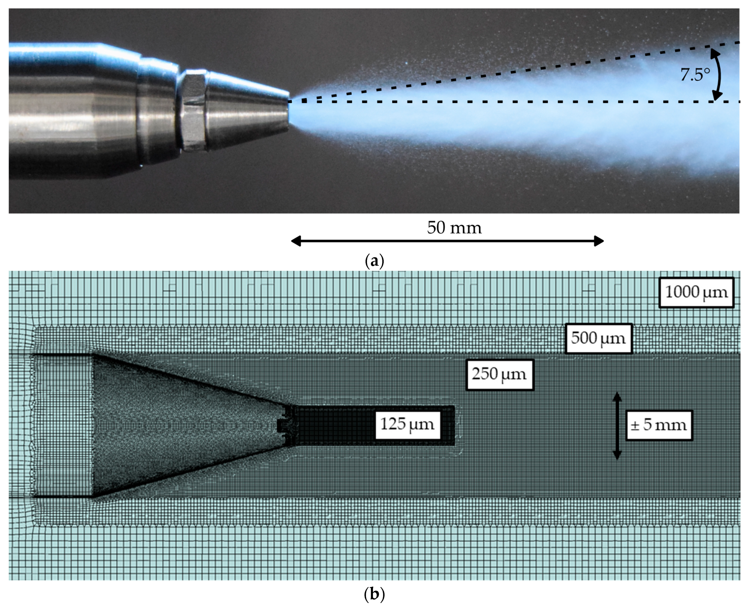
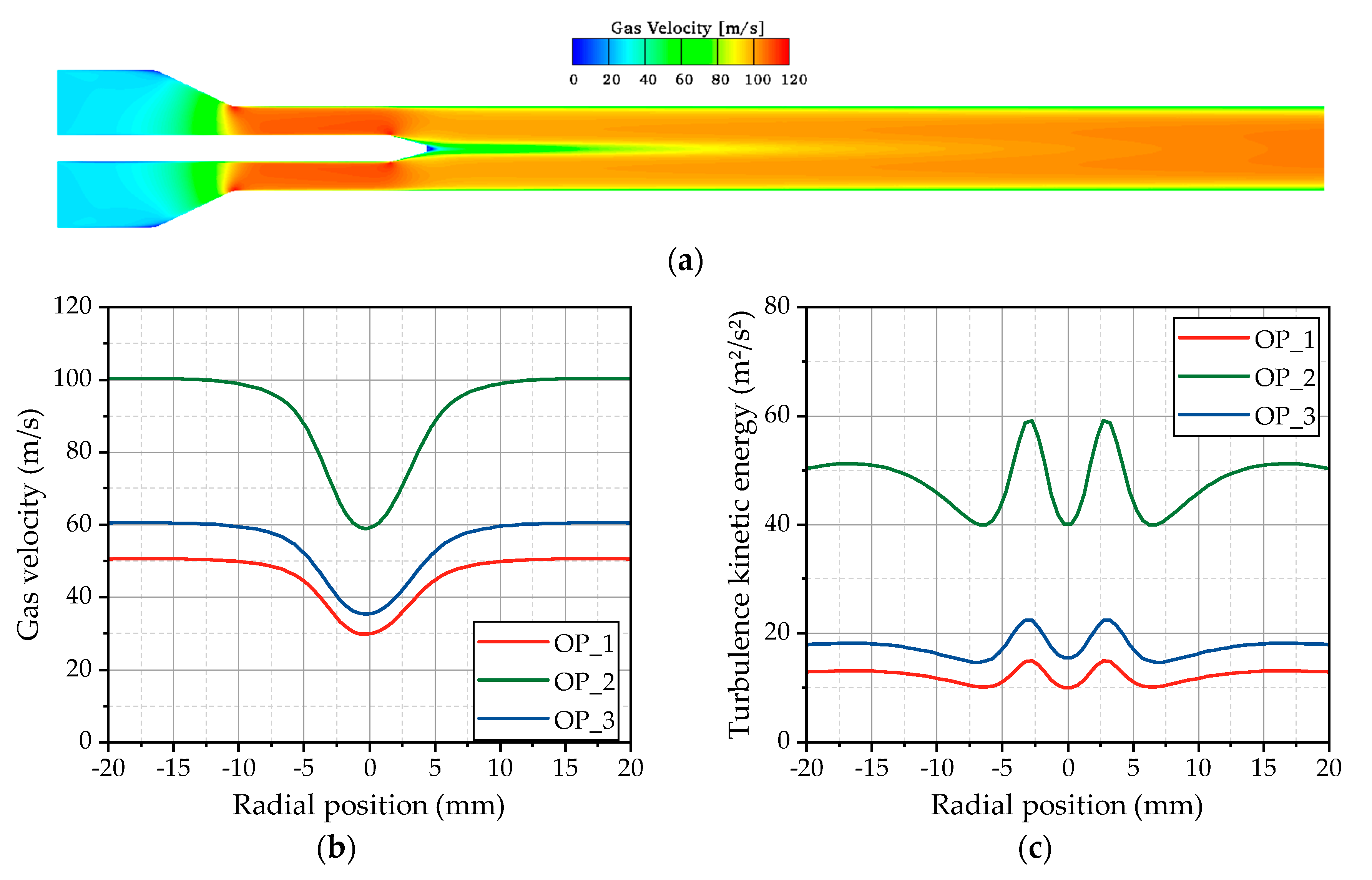
The simulations of the gas jet were carried out on the computational mesh shown in Figure 3. Before the gas jet is initialized, the hot gas flow in the test bench was calculated to provide a well-converged flow field. During these flow simulations, the time step is increased from 1 µs to 10 µs in order to speed up the calculation time. A resulting flow field is shown exemplarily for OP 2 in Figure 6a, whereby the gas velocity is illustrated on a plane cut through the center axis of the test bench. Downstream of the inlet of the computational domain, the gas is accelerated in the tapered cross section to velocities over 100 m/s. Passing the injector shaft mounted in the center of the pipe, the flow detaches from the injector cone and starts to recombine downstream of the nozzle exit. At the first measurement position, at a distance of 50 mm downstream, the nozzle the flow is still not completely recombined, resulting in the radial profiles of the gas velocity shown in Figure 6b. For OP 2, the velocity decreases from 100 m/s in the outer area to 60 m/s in the center of the pipe, which has to be considered for the evaluation of the gas jet and the spray characteristics. The velocity reduction is, for all operating points, in the range of 40%. Obviously, this velocity gradient is followed by the formation of a shear layer, which locally increases the turbulence. This behavior is clarified by the radial profiles of the turbulence kinetic energy depicted in Figure 6c. Thereby, two peaks are detectable ±3 mm away from the center axis, indicating the position of the shear layer. An unchanged position of these peaks can be found in all three operating points, even if the flow velocity and the turbulence level are completely different. The reason for these phenomena is the preservation of the Reynolds number by means of choosing the conditions for the hot gas flow by Lieber et al. [17].

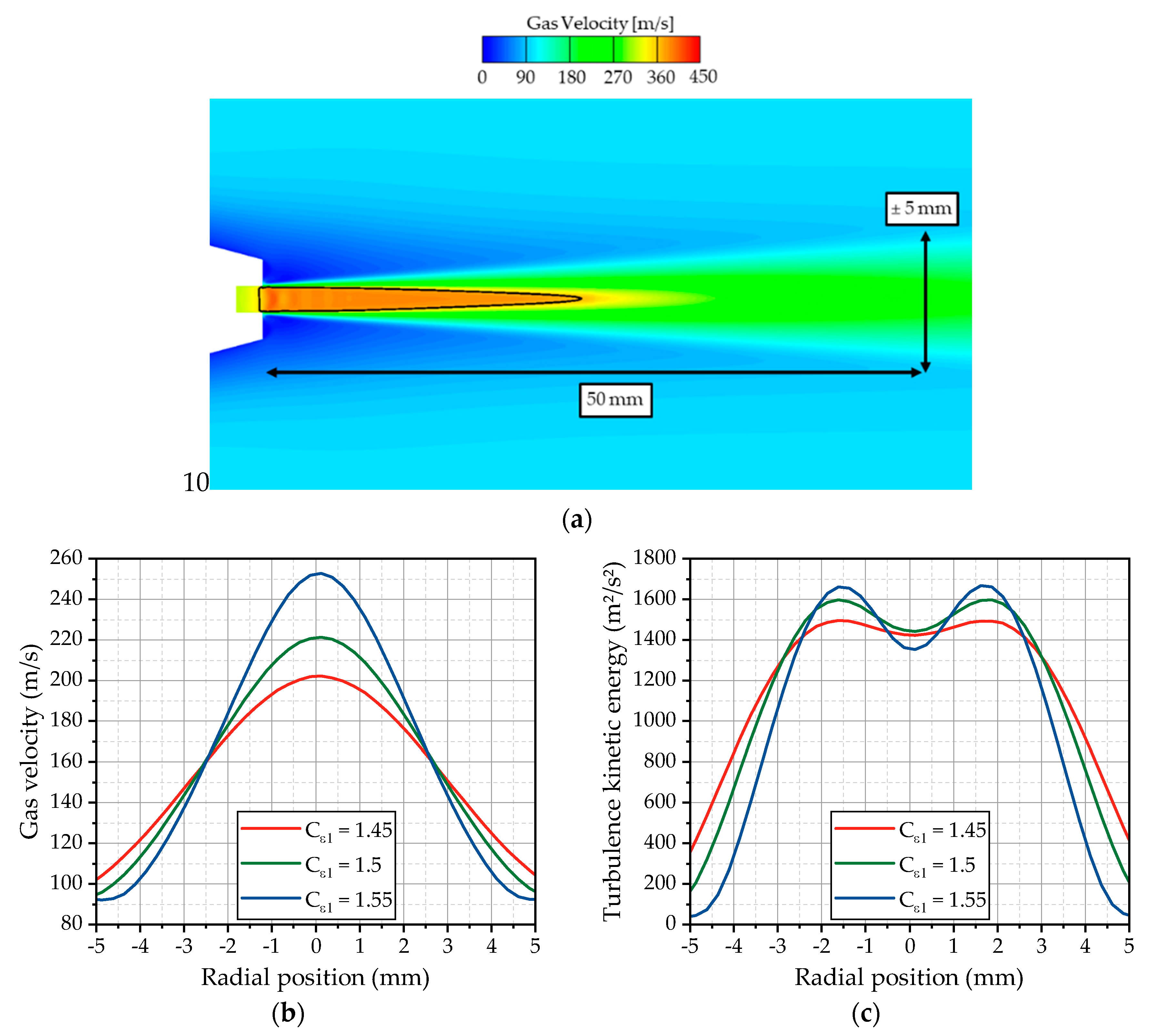
Starting from the simulations of the hot gas flow, the gas jet is initialized in the outflow channel of the nozzle. The gas flow inside the channel is in a subsonic state and accelerates to supersonic speed downstream of the nozzle exit, which is characteristic for under-expanded nozzles. Thereby, flow velocities over 400 m/s are present in the vicinity of the nozzle exit. The flow velocity on a plane cut through the center axis of the test bench and an isoline representing a Mach number (Ma) of one are depicted in Figure 7a. The expanding gas jet preserves a supersonic core up to 25 mm downstream the nozzle. Further downstream of the nozzle, the jet is rapidly decelerated on its center axis by radial momentum flux, leading to the widening of the radial velocity profile. The spreading rate determines the resulting velocity profile at the first measurement position and is strongly influenced by the choice of the turbulence model and the discretization.

For the investigation of the impact of the used k-ε turbulence model on the spreading rate, the model parameter C_ε1, which controls the influence of the production term P in the transport equation of the dissipation rate, is adjusted, as already discussed in Section 2.2.2. In Figure 7b, the velocity profiles for three different values of the C_ε1 parameter are plotted for OP 2. Obviously, the spreading rate of the jet is very sensitive to this parameter. Higher C_ε1 values lead to a smaller spreading rate and a narrower profile. Lower values result in a wider velocity profile. According to the fact that the standard k-ε model predicts a too-high spreading rate [25], the model constant C_ε1 is adapted to 1.49, which was found suitable to achieve a good agreement with the experimentally observed droplet velocities discussed in Section 3.2. The value of 1.49 is slightly lower than the often literature-proposed values of 1.55 and 1.6 [7,28]. Further on, the influence on the turbulence kinetic energy is investigated. The radial profiles of the turbulence kinetic energy are illustrated in Figure 7c for OP 2. For higher values of C_ε1, significant peaks appear at the radial positions ±1.5 mm, while, for lower values close to the standard model, the peaks seem to disappear. Lower values also lead to a wider spreading of the turbulence kinetic energy, which is consistent with the observations from the flow velocity.

3.2. Evaluation of Droplet Velocities

The following section covers the investigation of the droplet velocities derived from the experiment and the simulation. Thereby, the quality and the predictivity of the computational method will be discussed. Starting from the simulation of the gas jet, the droplets are released into the computational domain according to the initial conditions derived in Section 2.2.4. The droplet velocities were evaluated at the first measurement position 50 mm downstream of the nozzle exit in the radial direction. A traverse system was applied in the experiment to shift the measurement volume, starting from −5 mm to 5 mm, in 1 mm steps through the spray (see Section 2.1). Due to the higher signal-to-noise ratio, less droplets are detectable in the range of 0 mm to 5 mm, leading to less statistical significance and an asymmetric velocity profile. To overcome this, and to improve the comparability with the almost symmetric simulation data, the average of both sides is calculated and mirrored at the center axis [17].

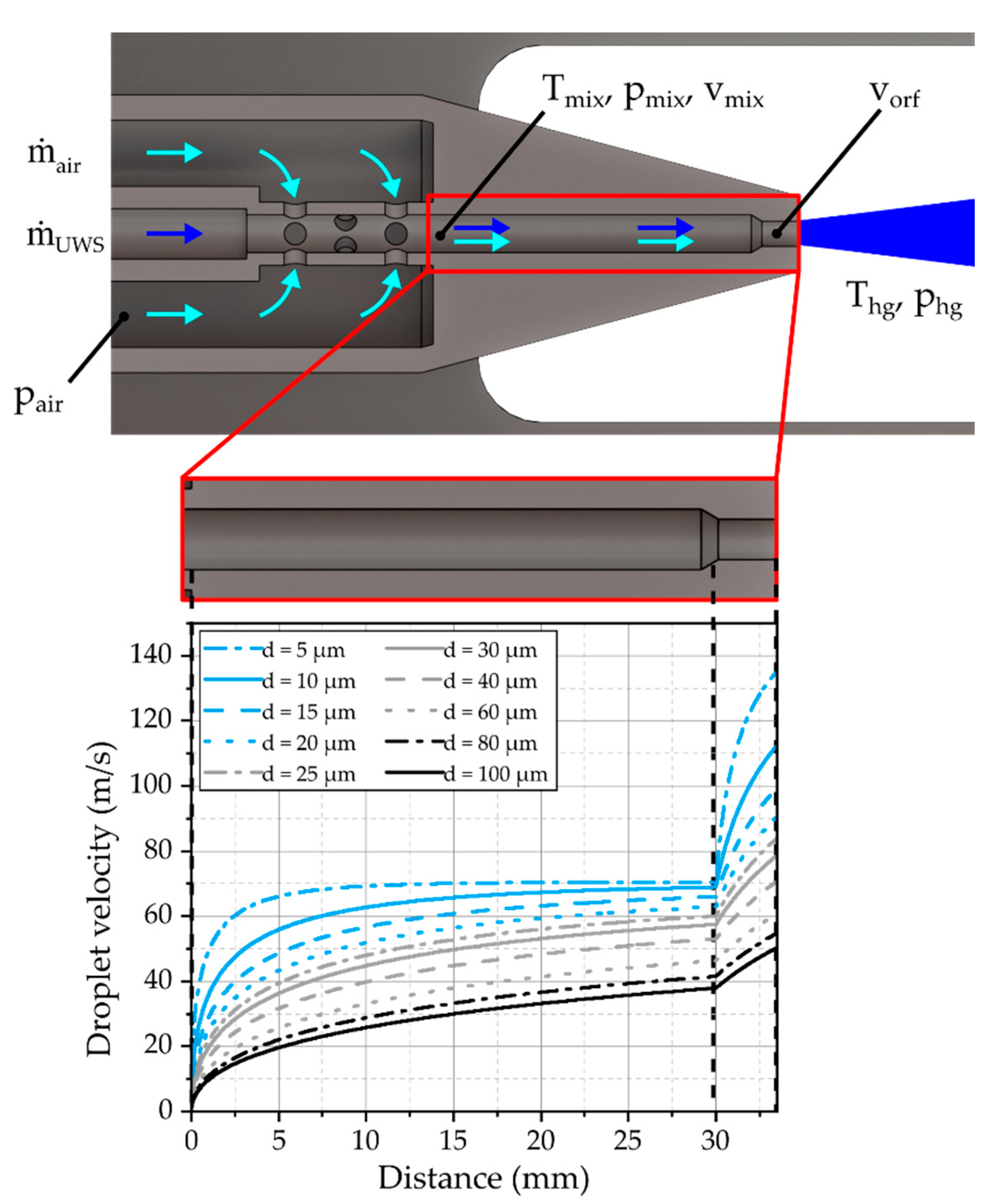
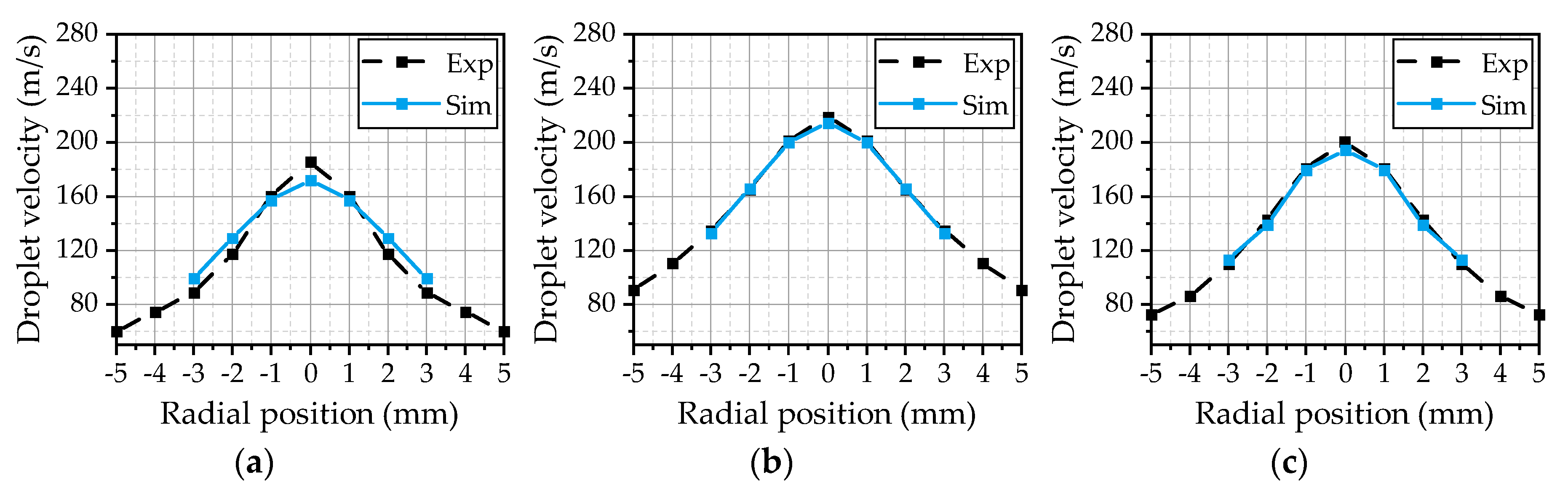
The spray data derived from the simulations is processed using a MATLAB^® (R2019b, The MathWorks, Inc., Natick, MA, USA) routine. Thereby, the data comprises the properties of every parcel in the simulation domain exported at different time steps. At first, the data is filtered to extract the parcels in the experimental measurement volume at the corresponding measurement positions. Subsequently, the temporal averages of the properties of different droplet size classes are calculated. This procedure is similar to the evaluation of the experimental data, where the derived values represent the temporal average of the detected droplets from the recorded images. The evaluated velocities of the droplets with a diameter of 5 µm for the three investigated operating points are illustrated in Figure 8. This size class is slightly above the smallest detectable droplet size of the experimental methodology and gives an insight into the gas velocity due to a small Stokes number. Overall, the simulation results are in a good agreement with the experiment for all three operating points. The best fit could be achieved for OP 2 (Figure 8b), which served as a reference point for the model calibration. Thus, the C_ε1 parameter of the turbulence model seems to be chosen appropriately. Starting from a maximum value at the center axis, the velocity decreases with the radial distance until it reaches the range of the gas velocity at ±5 mm. For OP 1 (Figure 8a), the simulated curve is a little wider than experimentally observed, resulting in a reduced maximum in the center. This may result from an overestimation of the spreading rate of the gas jet due to a higher gas mass flow and an increase of the ambient density from 0.54 kg/m³ (OP 2) to 1.08 kg/m³ (OP 1). Further on, there are no 5 µm droplets detected at the radial positions ±4 mm and ±5 mm in the simulation. This behavior is suspected to be a result of underestimated turbulent transport phenomena inside the spray, since the turbulent fluctuations are not resolved. Small droplets will follow the turbulent motion inside the spray plume, which distributes the droplets inside the spray. By means of RANS simulations, the turbulent dispersion is modeled as described in Section 2.2.3. due to the fact that RANS solutions provide an averaged flow field that contains no detailed information about the turbulent fluctuations. A deeper insight into the turbulent transport phenomena could be achieved using a large eddy simulation that resolves the largescale turbulence structures.

A further validation of the simulation is performed using the measured droplets with a diameter of 8 µm. These droplets possess a higher inertia and respond to an acceleration or a deacceleration of the gas flow with some delay. The radial velocity profiles of the droplets with a diameter of 8 µm are illustrated in Figure 9 for the three investigated operating points. The simulation results show a good correlation with the experimental data for all operating points, which suggests a predictivity of the model in the present range of the operating conditions. Droplets are also detected at a radial position of ±4 mm in the simulation. Thus, those droplets are less-aligned to the center of the spray by the high gas velocity inside the gas jet. However, at a radial position of ±5 mm, there are still no 8 µm droplets detectable in the simulation.

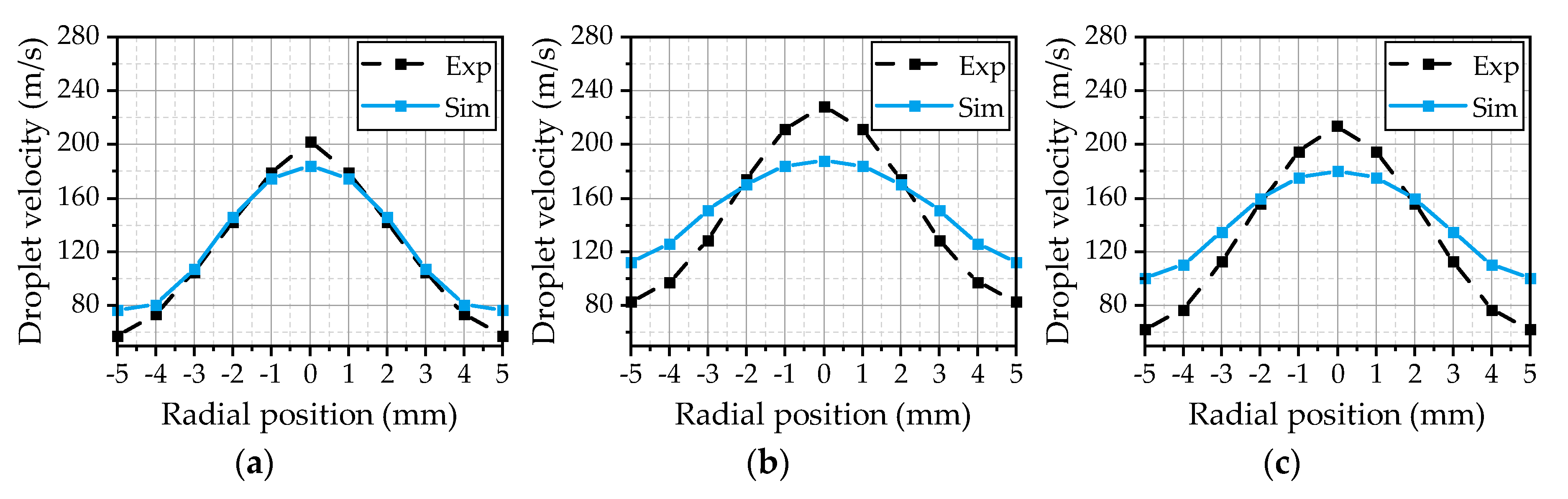
The velocity profiles of droplets with diameters greater than 15 µm are illustrated in Figure 10. These droplets represent large droplets in the present spray. In this case, the comparability of the simulation with the experiment is dependent on the conformity of the droplet spectra, due to the dependence of the droplet velocity on the droplet size. The simulated velocity profile for OP 1 (Figure 10a) is in a good agreement with the experimentally observed velocities. The maximum velocity in the center of the spray is slightly underpredicted. For OP 2 (Figure 10b) and OP 3 (Figure 10c), the velocity profile is predicted significantly wider by the simulation than in the experiment. This is followed by an overestimation of the droplet velocity in the outer area of the jet. The lower density of the hot gas in OP 2 and OP 3 results in a reduction of the momentum transfer between the gas phase and the liquid phase. This results in an underestimation of the deacceleration of larger droplets in the outer area and of the acceleration of larger droplets in the center of the spray.

One must consider the initial velocity imprinted on the droplets in the simulation for a more detailed interpretation of these phenomena. All droplets are initialized with a constant velocity. Imprinting the corresponding velocity for each size class on the initial droplets according to Section 2.2.4 may improve the results. This way, small droplets will emerge from the nozzle with a higher velocity, while larger droplets will emerge with a lower velocity. This will enhance the momentum transfer between the gas phase and larger droplets due to a reduction of the momentum flux to smaller droplets due to smaller relative velocities. Nevertheless, the estimated droplet initial conditions, in combination with the tuning of the turbulence model, provide reasonable results for a wide range of droplet sizes that are in good agreement with the experimentally determined velocity profiles.

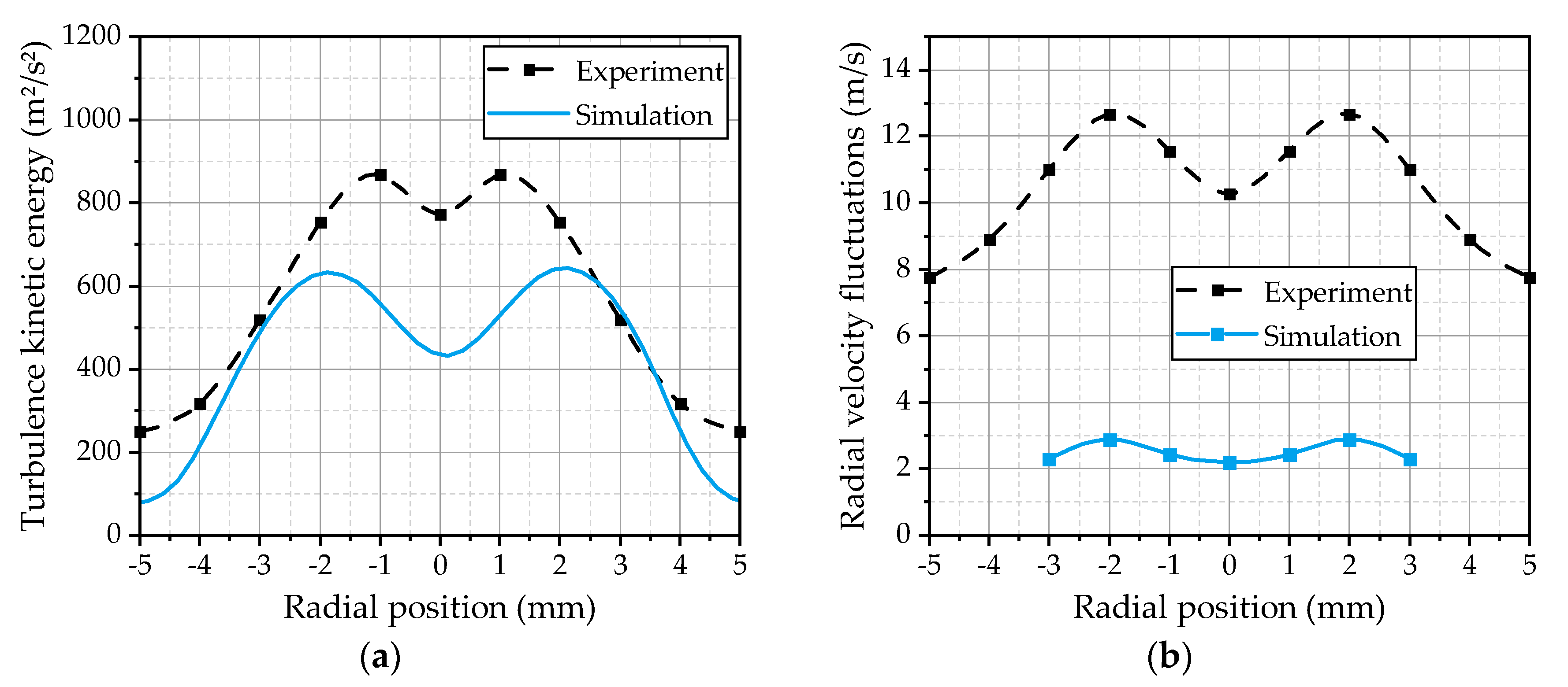
In addition to the mean velocities, the turbulent fluctuations inside the spray are of interest, because they represent the basis for the turbulent dispersion of the droplets. Further on, the turbulence enhances the heat and mass transfers, which increase the evaporation rate of the spray. Therefore, the turbulence kinetic energy calculated by the turbulence model in the gas phase is compared with the experimentally estimated turbulence kinetic energy from the velocity fluctuations of the 5 µm droplets. This droplet class can be used as an indicator for the turbulent fluctuations of the gas phase, as demonstrated in [17]. The radial profiles of the simulated and the experimentally evaluated turbulence kinetic energy at the first measurement position are depicted in Figure 11a. The shape of the two curves is qualitatively in a good agreement, while the absolute values in the center and the outer area of the spray are underestimated by the simulation. The contour of the simulated turbulence indicates that the value chosen for the C_ε1 parameter of the turbulence model is suitable. As shown in Figure 7c, the choice of C_ε1 strongly influences the profile of the turbulence kinetic energy. In addition, the radial components of the droplet velocity fluctuations are compared in Figure 11b. The simulation and the experimental results are represented by the velocity fluctuations of the 5 µm droplets. It becomes apparent that the velocity fluctuations of the droplets are much lower in the simulation, while the shapes of the two curves are qualitatively in good agreement. Even the position of the maxima is correctly predicted. This may be an indication of an underestimation of the turbulent dispersion effects inside the spray plume. One has also to consider that the information of the radial velocity fluctuations of the gas velocity is not provided by the RANS solution. Therefore, they have to be estimated by the turbulent dispersion model using the modeled turbulence kinetic energy, which will lead to uncertainties. More complex turbulence models like Reynolds stress models could be an interesting alternative for a more detailed modeling of the turbulent dispersion phenomena due to the fact that they are able to consider anisotropic turbulence. However, the turbulent transport inside the spray is a significant issue for further investigations.

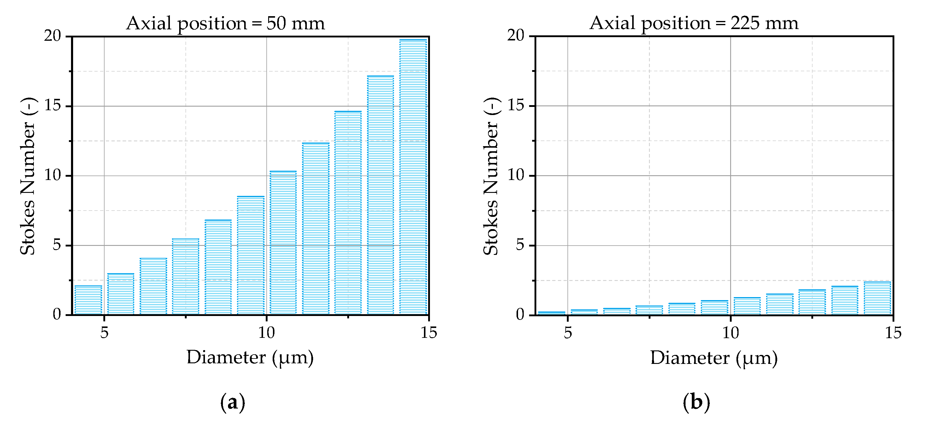
The Stokes number of the droplets is, as generally discussed in Section 2.2.3, a decisive parameter to evaluate a droplet’s response to the turbulent motion of the gas phase. Therefore, the Stokes number of the droplets is analyzed by means of the simulation results at the first two measurement positions downstream of the nozzle. Figure 12a illustrates the Stokes number as a function of the droplet size averaged in radial direction from -3 mm to 3 mm at the first measurement position. The radial positions are chosen due to the fact that there are still small droplets detectable, as previously discussed. The Stokes number increases with an increasing droplet diameter, which is mainly driven by a higher relaxation time due to a higher inertia of bigger droplets. The smallest droplets are in a range of a Stokes number of 2.5 and are, therefore, less affected by the turbulent motions of the gas phase, as expected. One reason for this behavior is the small eddy lifetime at this position. Further downstream the nozzle exit, the Stokes number decreases due to an increasing eddy lifetime, shown in Figure 12b for the second measurement position. At this position, the Stokes numbers of the smallest droplets are lower than unity, resulting in a high impact of the turbulent motion on the droplet trajectories. If the findings of Klose et al. [37] are considered, the Gosman and Ioannides model [31], applied for the modeling of the turbulent dispersion, provides good results in a narrow area of Stokes numbers ~2. The model should be able to describe the turbulent dispersion shortly after the first measurement position. In the area upstream the first measurement position, the Stokes numbers are higher, leading to uncertainties in the modeling. One has still to consider that, to finally judge the quality of the selected dispersion model, more detailed information about the initial conditions of the droplets at the nozzle exit is necessary.

3.3. Discussion of Droplet Sizes

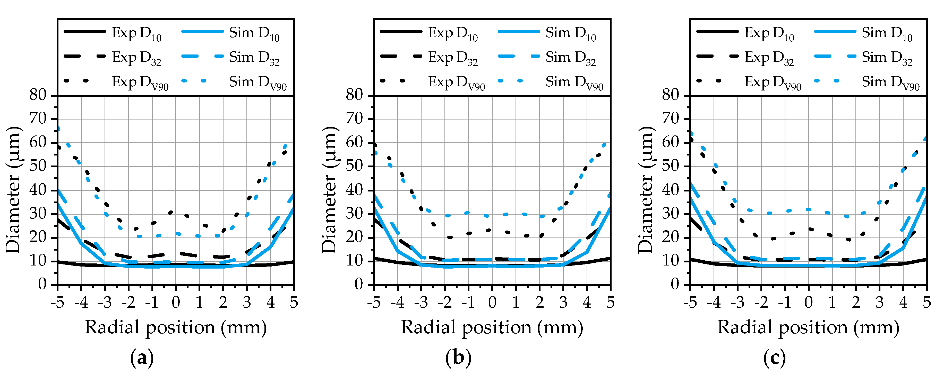
In addition to the droplet velocities, the diameter distribution of the spray is of interest for the assessment of the quality of the model. Therefore, the arithmetic diameter (D₁₀), the Sauter mean diameter (D₃₂) and diameter at the 90% volumetric quantile (D_V90), depicting the characteristic parameters of a droplet spectrum, are evaluated in the radial direction at the first measurement position 50 mm downstream of the nozzle. This is conducted by means of a MATLAB^® routine, as described in Section 3.2. The radial profiles of the characteristic parameters are plotted in Figure 13 for the three investigated operating points. The arithmetic diameter and the Sauter mean diameter calculated from the simulation data are in good agreement with the experimental data in the core region of the spray. In the outer area, starting from ±3 mm, the arithmetic diameter is overestimated by the model.

An explanation for this behavior is the absence of small droplets in this area as already presented in Figure 8. The Sauter mean diameter is in a range of 10 µm to 14 µm in the spray center for all three operating points, which confirms a continuously good atomization. The SMD is also correctly predicted by the model in the core zone, while it is overestimated in the outer area. Finally, the DV₉₀ from the simulation data is in a good agreement with the experiment over the whole radial distance for OP 1 (Figure 13a). For OP 2 (Figure 13b) and OP 3 (Figure 13c), there is a slight overestimation in the core area recognizable. 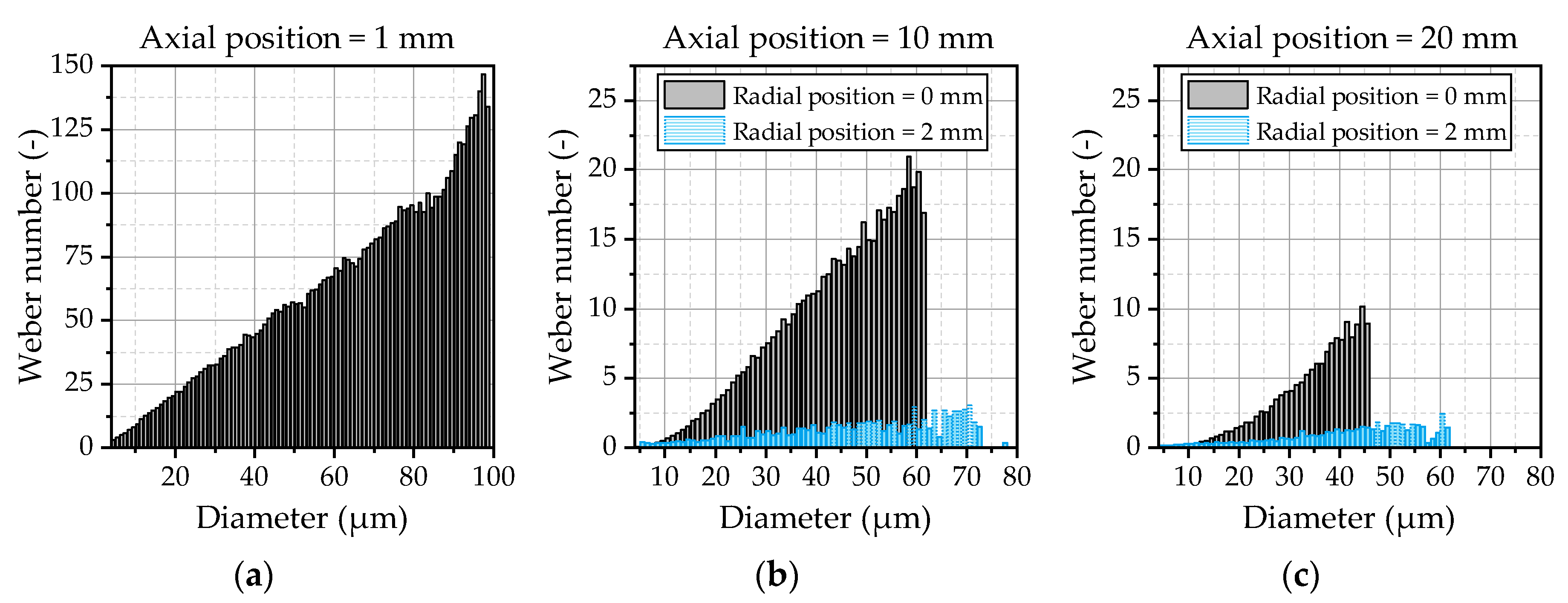The DV₉₀ depicts a sensitive parameter that can be strongly influenced by a small number of larger droplets. The correlation with the experimental data achieved by the model demonstrates that the droplet breakup and kinematics are predicted correctly. Large droplets emerging at the spray center are immediately broken up in the vicinity of the nozzle due to high relative velocities, while they persist in the outer area of the spray. This behavior can be analyzed by an evaluation of the Weber number of the droplets. The Weber number of the droplets at three different positions downstream of the nozzle exit is illustrated Figure 14. Further on, the Weber number is depicted in the spray center and the outer area of the spray at distances of 10 mm (Figure 14b) and 20 mm (Figure 14c) downstream the nozzle.

In the vicinity of the nozzle (Figure 14a), high Weber numbers up to 150 occur due to the high relative velocities of the droplets and the escaping gas jet. This results in an immediate breakup of the droplets that is also known from high-pressure injections. At the axial position of 20 mm (Figure 14c), the Weber numbers are smaller than 10, indicating that the main part of the secondary atomization is completed. The droplets in the outer area of the spray represented by the radial position of 2 mm in Figure 14b,c quickly leave the core region of the gas jet, resulting in Weber numbers smaller than 3 even for bigger droplets in the area of 50 µm to 70 µm. Those droplets are not atomized and are preserved at the spray boarders, resulting in the observed behavior of the DV₉₀ in Figure 13, which could be predicted quite well by the applied WAVE breakup model.

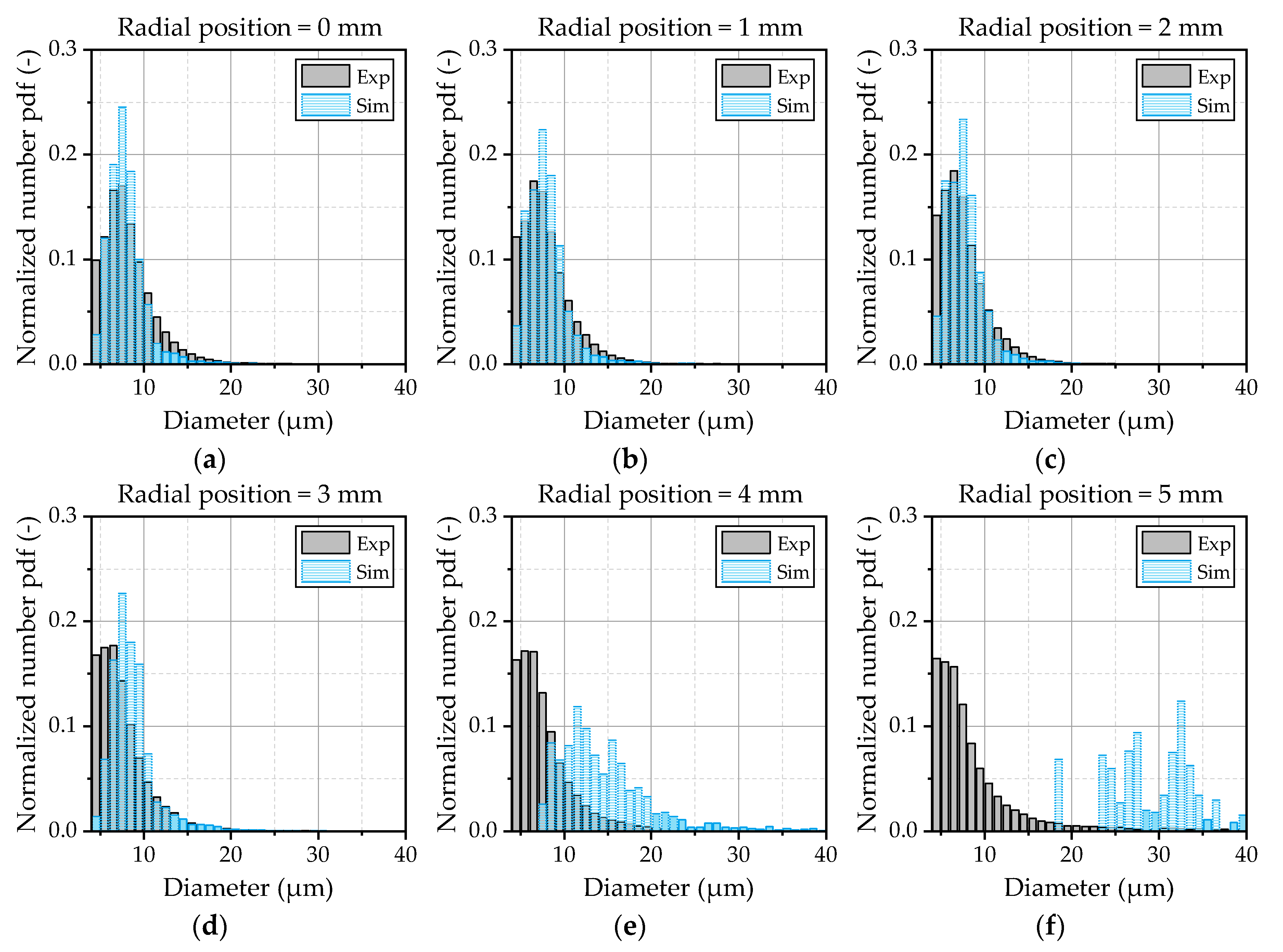
Apart from the characteristic parameters of the spray, the droplet spectra are evaluated in the following to get a deeper insight into the observed behavior of smaller droplets. Therefore, the filtered data from the simulation and the data of the single droplets detected in the experiment are processed with a MATLAB^® routine. Thus, the processing of the data is the same for the simulation and experiment, ensuring good comparability. One has to consider that the statistical significance of the experiment is considerably higher than of the simulation, due to the fact that the measured droplet spectrum at a given measurement position consists of 10⁴ to 10⁵ single droplets, which are represented by a few hundred to thousand detected parcels in the simulation. The droplet spectra at different radial positions are illustrated as number-based distributions in Figure 15 for OP 2.

In the center zone of the spray depicted by Figure 15a–c, the spectrum is well-predicted by the model. In the outer area, starting from 3 mm (Figure 15d) up to 5 mm (Figure 15f) the deviations between the experiment and simulation increased. The already discussed lack of small droplets at the edge of the spray cone becomes obvious by means of this illustration. Based on these results, further investigations should be conducted to get a deeper insight into the turbulent transport phenomena inside the jet and the breakup of the droplets inside the shear layer of the gas flow. Further on, a detailed investigation of the initial conditions of the droplets at the nozzle exit is necessary to provide well-defined boundary conditions for the validation of the turbulent dispersion. Thereby, large eddy simulations in combination with a volume-of-fluid approach could serve as a suitable method to gain detailed information about the turbulent structures and the formation of the initial droplets.

3.4. Evaporation of the Urea-Water Droplets

Prior to evaluating the predicted evaporation characteristics of the spray, the evaporation process of urea-water droplets will be discussed briefly. The evaporation can be subdivided into two main stages: The first stage is characterized by an almost exclusive evaporation of water. This means that there will be no evident difference between the evaporation of pure water and urea-water droplets. Once the water of the urea-water droplet is consumed by evaporation, the thermolysis and evaporation of urea sets in. This is the second stage, which can be described as an evaporation process with a considerably lower evaporation rate in comparison to water. At the same time, the droplet temperature increases drastically. A detailed investigation of the evaporation process of urea-water droplets is given by Birkhold [33].

The important conclusion from the brief discussion of the evaporation process is that a designated droplet size exists during the lifetime of each urea-water droplet at which, the evaporation rate is drastically reduced. This distinct feature of the evaporation process was used to define the droplet size at the limit of water evaporation as a criterion for determining the progress of spray evaporation in a previous study [17]. Using this criterion, the comparison of experimental results to numerical predictions is straightforward, which will be directly demonstrated in the following paragraphs.

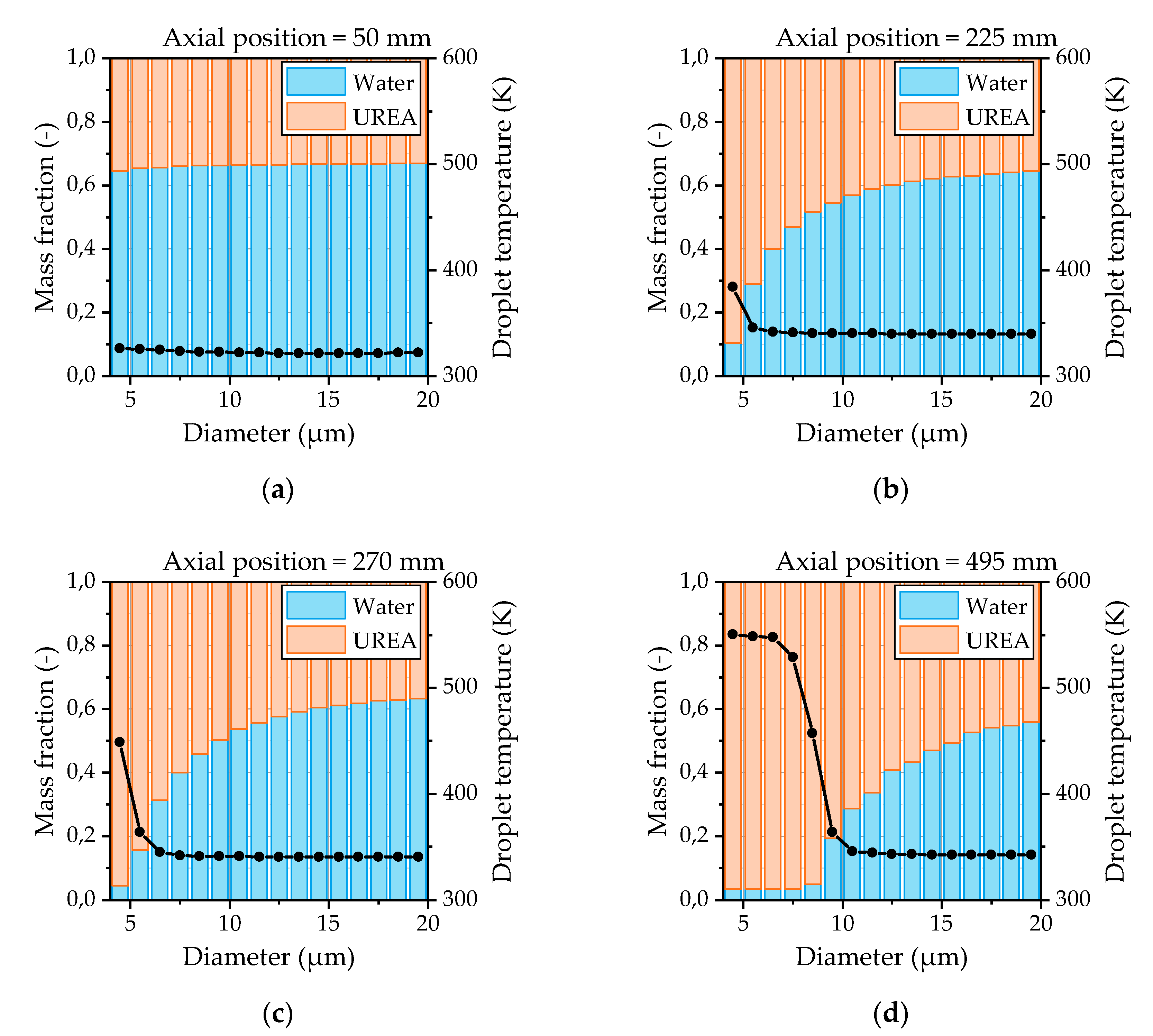
The evaporation characteristics of the urea-water droplets are evaluated from the simulations by means of the droplet temperature and the droplet composition. Thereby, the droplet composition provides information about whether a droplet undergoes water evaporation or urea thermolysis. The composition and temperatures of the droplets as a function of the droplet size and the distance from the nozzle are depicted in Figure 16 for OP 2. At the first measurement position shown in Figure 16a, there is no significant evaporation recognizable. Only the smallest droplets start to evaporate. This behavior also proves the suitability to apply an averaged droplet spectrum from the first measurement position as the initial condition at the nozzle exit in the CFD model. After the droplets are heated up, the water evaporation is present for almost all droplet sizes shown in Figure 16b. The urea thermolysis indicated by a rapid rise of the droplet temperature and a significant reduction of the water content has already begun for the smallest droplets at this position. Further downstream of the nozzle, the droplet diameter from which the urea thermolysis is present increases continuously, as illustrated in Figure 16c,d. Thereby, the droplet temperature reaches a steady state for droplets smaller than 7 µm at the last measurement position 495 mm downstream of the nozzle.

To compare the findings from the simulations with the experimental observations, the characteristic diameter at which the urea thermolysis starts is evaluated. The evaluation is conducted by the increase of the droplet temperature as a function of the droplet diameter. In the case of a strong rise above 10 K from size class to size class, the corresponding droplet size is determined as the diameter at the limit of water evaporation. The results are compared with the experimental data in Figure 17 for the three investigated operating points as a function of the axial distance from the nozzle. It is obvious that the progress of the evaporation process of the present urea-water spray is underpredicted by the model. The diameter at the limit of water evaporation is approximately 2 µm to 3 µm below the experimental results. Nevertheless, the effects of the three hot gas operating conditions are predicted correctly. The evaporation rate is significantly decreased from OP 1 to OP 2 due to a decrease in the ambient density. For OP 3, the evaporation rate is further decreased due to a considerably lower ambient temperature. The underestimation of the evaporation process in the simulations may be explained by the turbulent dispersion, which is quite lower in the simulations. The turbulent dispersion imprints an additional fluctuation velocity on the droplets, increasing the relative velocity of the droplets, which results in higher evaporation rates. Further on, the smallest droplets are more homogenously distributed over the spray plume, reducing the temperature decrease in the center of the spray in the experiment. However, to finally assess the observed deviations between the simulation and experiment, further investigations of the evaporation process are necessary.

4. Conclusions

In the present study, an air-assisted nozzle for the atomization of UWS has been modeled using a commercial CFD code. The model comprises the geometry of the hot gas test bench applied for the optical investigations that have provided the experimental droplet data to validate the model. The outflow channel of the atomizer is included in the computational mesh to correctly depict the boundary conditions of the emerging gas jet. A detailed modeling of the gas jet has been performed by an appropriate meshing strategy, with a cell size of 125 µm in the near nozzle region and an adjustment of the turbulence model to correct the spreading rate of the gas jet. A suitable droplet spectrum is derived from experimental results 50 mm downstream of the atomizer and imprinted on the initial droplets directly downstream of the nozzle exit. The initial velocity of the droplets is estimated by means of an analytical investigation of the two-phase flow inside the nozzle. Moreover, the numerical simulation is complemented by the WAVE breakup model in order to control the largest droplet size of the spray in regions of strong aerodynamic forces.

The experimental data is determined from microscopic shadowgraphs and provides correlations of the droplet size, velocity and radial position inside the spray plume. This data is used for a detailed validation of the CFD model. Thereby, the velocity profile of the droplets 50 mm downstream of the nozzle exit could be predicted quite accurately by the model for three different operating points with varying ambient conditions and compressed air mass flows. Thus, the model is able to capture the effects of the ambient density and initial momentum flux. The droplet sizes were also evaluated in the radial direction by the characteristic parameters D₁₀, D₃₂ and DV₉₀. The radial profile of the DV₉₀, which is quite sensitive to a small amount of large droplets, is predicted very well, indicating an appropriate selection of the initial conditions of the droplets and a good performance of the breakup model. Further on, this proves the suitability of the application of the modeling approach, which is also used in the case of cavitating diesel nozzles, in air-assisted atomizers.

In contrast to the experimental results, a considerable amount of small droplets is missing in the outer area of the spray. A deeper analysis of the droplet distribution inside the spray suggests an underestimation of the turbulent transport phenomena. This is confirmed by an investigation of the radial fluctuations of the droplet velocity, which are much lower in the simulation than in the experiment. As a consequence, the turbulent dispersion may be underestimated. However, to finally assess this topic further investigations of the turbulent dispersion model and the influence of the initial conditions of the droplets on the turbulent dispersion are necessary.

An analysis of the formation of the initial droplets by the process of a primary breakup would require a detailed simulation of the mixing chamber, which may be done by applying a large eddy simulation and a volume-of-fluid method. Further on, the LES is able to provide a deeper insight into the turbulent flow phenomena inside the spray. This could provide a more detailed basis for the evaluation and the adaption of the turbulent dispersion models to improve the RANS results.

Further investigations will be carried out to verify the droplet evaporation calculated by the CFD model. The experimental data further downstream of the nozzle will serve as a good starting point for the evaluation of the evaporation model. The first steps have already been taken to investigate the transition from water evaporation to urea thermolysis, serving promising results. However, due to the complex process of UWS preparation, there is still some effort needed to provide a well-suited model for the present case.

References

1. Johnson, T.V. Review of Diesel Emissions and Control. SAE Int. J. Fuels Lubr. 2010, 3, 16–29. [Google Scholar] [CrossRef]
2. Johnson, T.; Joshi, A. Review of Vehicle Engine Efficiency and Emissions. SAE Int. J. Engines 2018, 11, 1307–1330. [Google Scholar] [CrossRef]
3. Schlemmer-Kelling, U. Agenda 2030—Mega-Trends im Bereich der maritimen Großmotoren. In Heavy-Duty-, On- und Off-Highway-Motoren 2017, Effizienz und Emissionen: 12. Internationale MTZ-Fachtagung, Wiesbaden, 2018; Siebenpfeiffer, W., Ed.; Springer Vieweg: Wiesbaden, Germany, 2018; pp. 19–38. ISBN 978-3-658-21029-8. [Google Scholar]
4. Koebel, M.; Elsener, M.; Kleemann, M. Urea-SCR: A promising technique to reduce NOx emissions from automotive diesel engines. Catal. Today 2000, 59, 335–345. [Google Scholar] [CrossRef]
5. Fischer, S.; Bitto, R.; Lauer, T.; Krenn, C.; Tauer, J.; Pessl, G. Impact of the Turbulence Model and Numerical Approach on the Prediction of the Ammonia Homogenization in an Automotive SCR System. SAE Int. J. Engines 2012, 5, 1443–1458. [Google Scholar] [CrossRef]
6. Payri, R.; Bracho, G.; Gimeno, J.; Moreno, A. Investigation of the urea-water solution atomization process in engine exhaust-like conditions. Exp. Therm. Fluid Sci. 2019, 108, 75–84. [Google Scholar] [CrossRef]
7. Merker, G.P.; Teichmann, R. Grundlagen Verbrennungsmotoren; Springer Fachmedien: Wiesbaden, Germany, 2018; ISBN 978-3-658-19211-2. [Google Scholar]
8. Spiteri, A.; Dimopoulos Eggenschwiler, P.; Liao, Y.; Wigley, G.; Michalow-Mauke, K.A.; Elsener, M.; Kröcher, O.; Boulouchos, K. Comparative analysis on the performance of pressure and air-assisted urea injection for selective catalytic reduction of NOx. Fuel 2015, 161, 269–277. [Google Scholar] [CrossRef]
9. Liao, Y.; Eggenschwiler, P.D.; Spiteri, A.; Nocivelli, L.; Montenegro, G.; Boulouchos, K. Fluid Dynamic Comparison of AdBlue Injectors for SCR Applications. SAE Int. J. Engines 2015, 8, 2303–2311. [Google Scholar] [CrossRef]
10. Lauer, T. Preparation of Ammonia from Liquid AdBlue—Modeling Approaches and Future Challenges. Chem. Ing. Tech. 2018, 90, 783–794. [Google Scholar] [CrossRef]
11. Zheng, G.; Wang, F.; Zhang, S.; Zhang, J.; Tao, J.; Zhao, Z.; Fan, J. Development of Compact SCR Systems with Closely Coupled Injector Configurations. SAE Tech. Pap. 2014, 1, 1546. [Google Scholar] [CrossRef]
12. Hua, L.; Zhao, Y.-g.; Hu, J.; Tao, T.; Shuai, S.-J. Comparison between Air-Assisted and Airless Urea Spray for Diesel SCR System by PDA and CFD. SAE Tech. Pap. 2012, 1, 1081. [Google Scholar] [CrossRef]
13. Nishad, K.; Ries, F.; Janicka, J.; Sadiki, A. Analysis of spray dynamics of urea–water-solution jets in a SCR-DeNOx system: An LES based study. Int. J. Heat Fluid Flow 2018, 70, 247–258. [Google Scholar] [CrossRef]
14. Edelbauer, W.; Birkhold, F.; Rankel, T.; Pavlović, Z.; Kolar, P. Simulation of the liquid break-up at an AdBlue injector with the volume-of-fluid method followed by off-line coupled Lagrangian particle tracking. Comput. Fluids 2017, 157, 294–311. [Google Scholar] [CrossRef]
15. Chen, M.; Williams, S. Modelling and Optimization of SCR-Exhaust Aftertreatment Systems. SAE Tech. Pap. 2005, 1, 0969. [Google Scholar] [CrossRef]
16. Naik, A.; Höltermann, M.; Lauer, E.; Blodig, S.; Dinkelacker, F. Modeling of an Air-Assisted Spray Breakup of Urea-Water Solution for SCR Applications. In Proceedings of the 4th World Congress on Momentum, Heat and Mass Transfer, Rome, Italy, 10–12 April 2019; Avestia Publishing: Orléans, ON, Canada, 2019. [Google Scholar]
17. Lieber, C.; Koch, R.; Bauer, H.-J. Microscopic Imaging Spray Diagnostics under High Temperature Conditions: Application to Urea–Water Sprays. Appl. Sci. 2019, 9, 4403. [Google Scholar] [CrossRef] [Green Version]
18. Lieber, C.; Koch, R.; Bauer, H.-J. Spray evaporation of urea–water solution: Experiments and modelling. Exp. Therm. Fluid Sci. 2020, 116, 110108. [Google Scholar] [CrossRef]
19. Ström, H.; Lundström, A.; Andersson, B. Choice of urea-spray models in CFD simulations of urea-SCR systems. Chem. Eng. J. 2009, 150, 69–82. [Google Scholar] [CrossRef]
20. Sovani, S.D.; Sojka, P.E.; Lefebvre, A.H. Effervescent atomization. Prog. Energy Combust. Sci. 2001, 27, 483–521. [Google Scholar] [CrossRef]
21. Li, Y.; Kirkpatrick, A.; Mitchell, C.; Willson, B. Characteristic and Computational Fluid Dynamics Modeling of High-Pressure Gas Jet Injection. J. Eng. Gas Turbines Power 2004, 126, 192–197. [Google Scholar] [CrossRef]
22. Abraham, J. What is Adequate Resolution in the Numerical Computations of Transient Jets? J. Engines 1997, 106, 141–155. [Google Scholar]
23. Franquet, E.; Perrier, V.; Gibout, S.; Bruel, P. Free underexpanded jets in a quiescent medium: A review. Prog. Aerosp. Sci. 2015, 77, 25–53. [Google Scholar] [CrossRef]
24. AVL List GmbH. CFD Solver—AVL FIRE.; Version 2018.1; AVL List GmbH: Graz, Austria, 2018. [Google Scholar]
25. Yoder, D.A.; DeBonis, J.R.; Georgiadis, N.J. Modeling of Turbulent Free Shear Flows. In Proceedings of the 21st AIAA Computational Fluid Dynamics Conference, San Diego, CA, USA, 24–27 June 2013; American Institute of Aeronautics and Astronautics: Reston, VA, USA, 2013; p. 06242013. [Google Scholar]
26. McGuirk, J.J.; Rodi, W. The Calculation of Three-Dimensional Turbulent Free Jets. In Turbulent Shear Flows I: Selected Papers from the First International Symposium on Turbulent Shear Flows; Durst, F., Launder, B.E., Schmidt, F.W., Whitelaw, J.H., Eds.; Springer: Berlin/Heidelberg, Germany, 1979; pp. 71–83. ISBN 978-3-642-46397-6. [Google Scholar]
27. Pope, S.B. An explanation of the turbulent round-jet/plane-jet anomaly. AIAA J. 1978, 16, 279–281. [Google Scholar] [CrossRef]
28. Dally, B.B.; Fletcher, D.F.; Masri, A.R. Flow and mixing fields of turbulent bluff-body jets and flames. Combust. Theory Model. 1998, 2, 193–219. [Google Scholar] [CrossRef]
29. Graham, L.J.W.; Bremhorst, K. Application of the k–ε Turbulence Model to the Simulation of a Fully Pulsed Free Air Jet. J. Fluids Eng. 1993, 115, 70–74. [Google Scholar] [CrossRef]
30. Stiesch, G. Modeling Engine Spray and Combustion Processes; Springer: Berlin/Heidelberg, Germany, 2003; ISBN 9783662087909. [Google Scholar]
31. Gosman, A.D.; loannides, E. Aspects of Computer Simulation of Liquid-Fueled Combustors. J. Energy 1983, 7, 482–490. [Google Scholar] [CrossRef]
32. Liu, A.B.; Mather, D.; Reitz, R.D. Modeling the Effects of Drop Drag and Breakup on Fuel Sprays. J. Engines 1993, 102, 83–95. [Google Scholar]
33. Birkhold, F. Selektive Katalytische Reduktion von Stickoxiden in Kraftfahrzeugen. Untersuchung der Einspritzung von Harnstoffwasserlösung. Ph.D. Thesis, University of Karlsruhe, Karlsruhe, Germany, 2007. [Google Scholar]
34. Abramzon, B.; Sirignano, W.A. Droplet vaporization model for spray combustion calculations. Int. J. Heat Mass Transf. 1989, 32, 1605–1618. [Google Scholar] [CrossRef]
35. Halonen, S.; Kangas, T.; Haataja, M.; Lassi, U. Urea-Water-Solution Properties: Density, Viscosity, and Surface Tension in an Under-Saturated Solution. Emiss. Control Sci. Technol. 2017, 3, 161–170. [Google Scholar] [CrossRef]
36. Tropea, C. Optical Particle Characterization in Flows. Annu. Rev. Fluid Mech. 2011, 43, 399–426. [Google Scholar] [CrossRef] [Green Version]
37. Klose, G.; Rembold, B.; Koch, R.; Wittig, S. Comparison of state-of-the-art droplet turbulence interaction models for jet engine combustor conditions. Int. J. Heat Fluid Flow 2001, 22, 343–349. [Google Scholar] [CrossRef]
Figure 1. (a) Picture of the experimental setup for investigation of urea-water sprays under high temperature and pressure conditions and (b) the schematic of the test section and the utilized diagnostics adapted from [17].
Applsci 10 05723 g001
Figure 2. Schematic diagram of the air-assisted atomizer with an inner mixing chamber.
Applsci 10 05723 g002
Figure 3. (a) Spray image of the near nozzle area taken from the experiment. (b) Local mesh refinements of the computational mesh in the near nozzle area with corresponding cell sizes and identification of the radial range of the first measurement position.
Applsci 10 05723 g003
Figure 4. (a) Schematic of the experimental measurement positions and representative cross section areas of the spray cone. (b) Droplet diameter distributions measured at different radial distances from the center line of the spray, and (c) spatially averaged and corrected droplet diameter distributions.
Applsci 10 05723 g004
Figure 5. Estimation of the velocity of droplets of different size at the atomizer exit.
Applsci 10 05723 g005
Figure 6. (a) Velocity of the bulk gas flow for OP 2 shown on a plane cut through the center line of the test rig. (b) Gas velocity and (c) turbulence kinetic energy over the radial position for the three selected operating points at the first measurement position downstream of the atomizer.
Applsci 10 05723 g006
Figure 7. (a) Velocity of the gas jet and isoline with Ma = 1 (black line) for OP 2, with Cε1 = 1.5 shown on a plane cut through the center line of the test rig. (b) Gas velocity and (c) turbulence kinetic energy over the radial position for the three selected parameters of the k-ε turbulence model for OP 2 at the first measurement position.
Applsci 10 05723 g007
Figure 8. Simulated and measured radial velocity profiles of droplets with a diameter of 5 µm for OP 1 (a), OP 2 (b) and OP 3 (c).
Applsci 10 05723 g008
Figure 9. Simulated and measured radial velocity profiles of droplets with a diameter of 8 µm for OP 1 (a), OP 2 (b) and OP 3 (c).
Applsci 10 05723 g009
Figure 10. Simulated and measured radial profiles of the mean droplet velocity for all droplets with a diameter greater than 15 µm for OP 1 (a), OP 2 (b) and OP 3 (c).
Applsci 10 05723 g010
Figure 11. (a) Simulated and measured radial profiles of the turbulence kinetic energy calculated from the fluctuations of the corresponding velocity components of the droplets for the experiment and from the gas phase turbulence for the simulation. (b) Radial velocity fluctuations calculated from the fluctuations of the corresponding velocity components of the droplets for both the simulation and experiment.
Applsci 10 05723 g011
Figure 12. Stokes number of the simulated droplets as a function of the droplet diameter 50 mm (a) and 225 mm (b) downstream the nozzle exit averaged over the radial distance from −3 mm to 3 mm.
Applsci 10 05723 g012
Figure 13. Arithmetic diameter, Sauter mean diameter and diameter at the 90% volumetric quantile in the radial direction for OP 1 (a), OP 2 (b) and OP 3 (c).
Applsci 10 05723 g013
Figure 14. Droplet Weber number as function of the droplet diameter for OP 2 in the vicinity of the nozzle (a) 10 mm (b) and 20 mm (c) downstream of the nozzle exit.
Applsci 10 05723 g014
Figure 15. Normalized number-based droplet distribution for OP 2 at the first measurement position in a radial distance of 0 mm (a); 1 mm (b); 2 mm (c); 3 mm (d); 4 mm (e) and 5 mm (f).
Applsci 10 05723 g015
Figure 16. Droplet composition depicted by the mass fractions of urea and water as a function of the droplet size with the corresponding droplet temperature in an axial distance of 50 mm (a), 225 mm (b), 270 mm (c) and 495 mm (d) downstream of the nozzle.
Applsci 10 05723 g016
Figure 17. Droplet size at the limit of water evaporation as a function of the axial distance from the nozzle for the three investigated operating points.
Applsci 10 05723 g017