A Methodology for Increasing Convergence Speed of Traffic Assignment Algorithms Based on the Use of a Generalised Averaging Function

Abstract

In this paper, we propose a generalisation of the Method of Successive Averages (MSA) for solving traffic assignment problems. The generalisation consists in proposing a different step sequence within the general MSA framework to reduce computing times. The proposed step sequence is based on the modification of the classic 1/k sequence for improving the convergence speed of the algorithm. The reduction in computing times is useful if the assignment problems are subroutines of algorithms for solving Network Design Problems—such algorithms require estimation of the equilibrium traffic flows at each iteration, hence, many thousands of times for real-scale cases. The proposed algorithm is tested with different parameter values and compared with the classic MSA algorithm on a small and on two real-scale networks. A test inside a Network Design Problem is also reported. Numerical results show that the proposed algorithm outperforms the classic MSA with reductions in computing times, reaching up to 79%. Finally, the theoretical properties are studied for stating the convergence of the proposed algorithm.

1. Introduction

The equilibrium traffic assignment problem has been widely studied since the early 1950s [1], both with respect to theoretical properties and proposing solution methods and algorithms. The Method of Successive Averages (MSA) is one of the most commonly used algorithms for solving the problem; it was proposed by References [2,3], and its convergence was stated by Reference [4]. The MSA proposed by References [2,3] operates on link flows (MSA-FA). On the other hand, Reference [5] proposed the MSA-CA which operates on link costs; while, Reference [6] devised the MSA-ACO based on Ant Colony Optimisation. Solution algorithms in the case of elastic demand were proposed and analysed by References [5,7,8].

The MSA algorithm at each iteration, k, averages the traffic flows calculated by stochastic uncongested network loading, with weight 1/k, with the results of the previous iteration, with weight (k–1)/k. Alternative step sequences (or weighting methods) were proposed, among others, by References [9,10,11]. More recently, Reference [12] proposed three revised versions of the traditional MSA method, namely: (i) Restarting MSA (RMSA), where the iteration counter is re-initialised after a specific number of iterations; (ii) Double RMSA (R2MSA), where the iteration counter is re-initialised to a variable value; (iii) Weighted MSA (WMSA), based on the self-regulated averaging method proposed by Reference [13] for solving the stochastic user equilibrium problem. The above-mentioned MSA schemes have been adopted by Reference [14] for solving a stochastic frequency-based assignment considering pre-trip/en-route path choice behaviour. Similarly, Reference [15], which extended the approach proposed in Reference [16], compared different MSA-based resolution techniques in the case of a stochastic assignment with multi-vehicle types (i.e., connected, automated, and autonomous vehicles, as well as traditional ones).

A generalisation of the averaging procedure, not limited to the traffic assignment problem, was provided by Reference [17]; while, Reference [18] proposed a refresh memory method for solving the combined assignment-control problem.

With the computing capabilities of modern PCs, the solution time of the traffic assignment problem is fairly short, also for large-size networks, if the problem has to be solved only once or a few times. Network Design Problems (NDPs) are usually solved by adopting procedures that use assignment algorithms as subroutines (bi-level approach); some reviews on NDPs can be found in References [19,20,21,22]. Indeed, for evaluating the objective function corresponding to a solution to the NDP, it is necessary to estimate traffic flows on the network. In this case, in most approaches, the assignment problem has to be solved a number of times equal to the solutions examined by the NDP algorithm; hence, several thousands of times in real-scale applications. Therefore, reducing the computing time of assignment algorithms is an important target since it may lead to a significant reduction in computing times for solving NDPs. In this context, Reference [23] proposed an MSA-based algorithm acting on the traffic flows adopted in the initialisation phases for reducing calculation times of NDPs when the topology of the network configuration remains unchanged.

With respect to the previous literature, in this paper we propose a new method that adopts a variant to the MSA algorithm: It is based on a parameter that can be set for each network to minimise the computing time. Moreover, in order to show its promising performance, it has been compared to other methods proposed in the literature. Finally, after the setting phase, the algorithm can be included within the NDP algorithm, minimising the whole computing time for solving the problem.

The remaining part of the paper is organised as follows: Section 2 introduces the model formulation; the proposed algorithm is analysed in Section 3, and Section 4 summarises the numerical results; Section 5 concludes the paper and outlines the research prospects. In Appendix A the convergence of the proposed algorithm is stated, and Appendix B presents a comparison with some MSA-based algorithms is provide. In Appendix C and Appendix D, the Network Design Problem and the algorithm used for its solution in the numerical test are illustrated.

2. Model Formulation

The traffic assignment problem consists of estimating traffic flows on a transportation network. In order to solve this problem, we need three elements: the travel demand (summarised in an Origin-Destination matrix), the transportation supply (modelled with a supply model) and the user path choice behaviour (modelled with a path choice model). Several models can be used for solving the problem depending on the transportation system (road network, mass-transit network, multimodal transportation network, etc.), the assumptions on the travel demand (fixed or variable), the approach to studying the interactions between demand and supply (user equilibrium or dynamic approach), the dependence or otherwise of link costs on flows (uncongested or congested), the assumption on the route choice model (deterministic or stochastic), and so forth. An in-depth analysis of traffic assignment models can be found elsewhere (see, for instance, Reference [24]). Even if the proposed algorithm can also be used to solve other assignment problems, in this paper, we consider the congested road network, fixed demand, user equilibrium approach and stochastic route choice model.

On a road network, the link flow vector, f, once the transport demand has been fixed, depends on link costs, and hence, on the link cost vector, c:

f = φ(c)

(1)

with:

φ(c) = AP(A^Tc) d

where A is the link-path incidence matrix, whose components, a_lp, are equal to 1 if link l belongs to path p and 0 otherwise; P is the path choice probability matrix, with a column for each od pair and a row for each path p; the generic element, P_p,od, of this matrix represents the probability that a user will use path p from origin o to destination d (if path p does not connect the od pair, P_p,od is equal to 0); d is the demand vector, whose components are the demand values d_od for each od pair.

The generic cost, c_l, of link l can be assumed dependent only on the flow on the same link, f_l.

Formally, we can write:

c = χ(f)

(2)

Substituting (2) in (1), we obtain the following:

f = φ(χ(f))

(3)

which relates flows, f, and costs, c. Equation (3) is a fixed-point problem; the solution is represented by the equilibrium traffic flows, f*, which is congruent with the corresponding link costs, c = χ(f*).

Formally, we can write:

f* = φ(χ(f*))    or   f* = A P(A^Tχ(f*)) d

(4)

In this case, it may be stated, under some assumptions, that the solution to the fixed-point problem (4) exists and is unique [5] and that the MSA algorithm converges to it [4].

3. Solution Algorithm

In order to solve the fixed-point problems (4) we propose an algorithm based on the MSA general framework. The first formulation of MSA [2] generates a succession of feasible link flow vectors, f ^k, starting from an initial solution (usually f ⁰ = 0). At each iteration k, the solution f^k is generated by combining traffic flows obtained by a Stochastic Uncongested Network (SUN) assignment, f_SUN^k = φ_SUN(c^k), with the previous solution, f ^k−1

At each iteration k, in order to generate the solution f^k, the results of the SUN assignment, f_SUN^k, are averaged, with weight 1/k, with the results of the previous iteration, f ^k−1, with weight (k − 1)/k:

f^k = ((k − 1)/k) · f ^k−1 + (1/k) · f_SUN^k

(5)

that is:

f^k = f ^k−1 + 1/k (f_SUN^k− f ^k−1)

(6)

Since the algorithm works directly on flows, it is also known as MSA-FA (Flow Averaging). Algorithm 1 reports the code of the traditional MSA-FA algorithm, where ε represents the stop threshold.

Algorithm 1 Traditional MSA-FA algorithm

1:   k = 0 2:   f0 = 0 3:   do while |fSUNk − f k−1|/f k−1 ≥ ε 4:   k = k + 1 5:   ck = χ(f k−1) 6:   fSUNk = φSUN(ck) 7:   fk = f k−1 + 1/k · (fSUNk − f k−1) 8:   loop 9:   f * = fk 10:   end

It is worth noting that the averages applied to the flows belonging to successive iterations have to be considered an algorithmic trick and should not be confused with the weights that simulate the learning process in the dynamic assignment models. Indeed, the MSA algorithms apply to stationary models, while the simulation of learning processes (comparison between expected and experienced performances) are typical of day-to-day dynamics models [24,25].

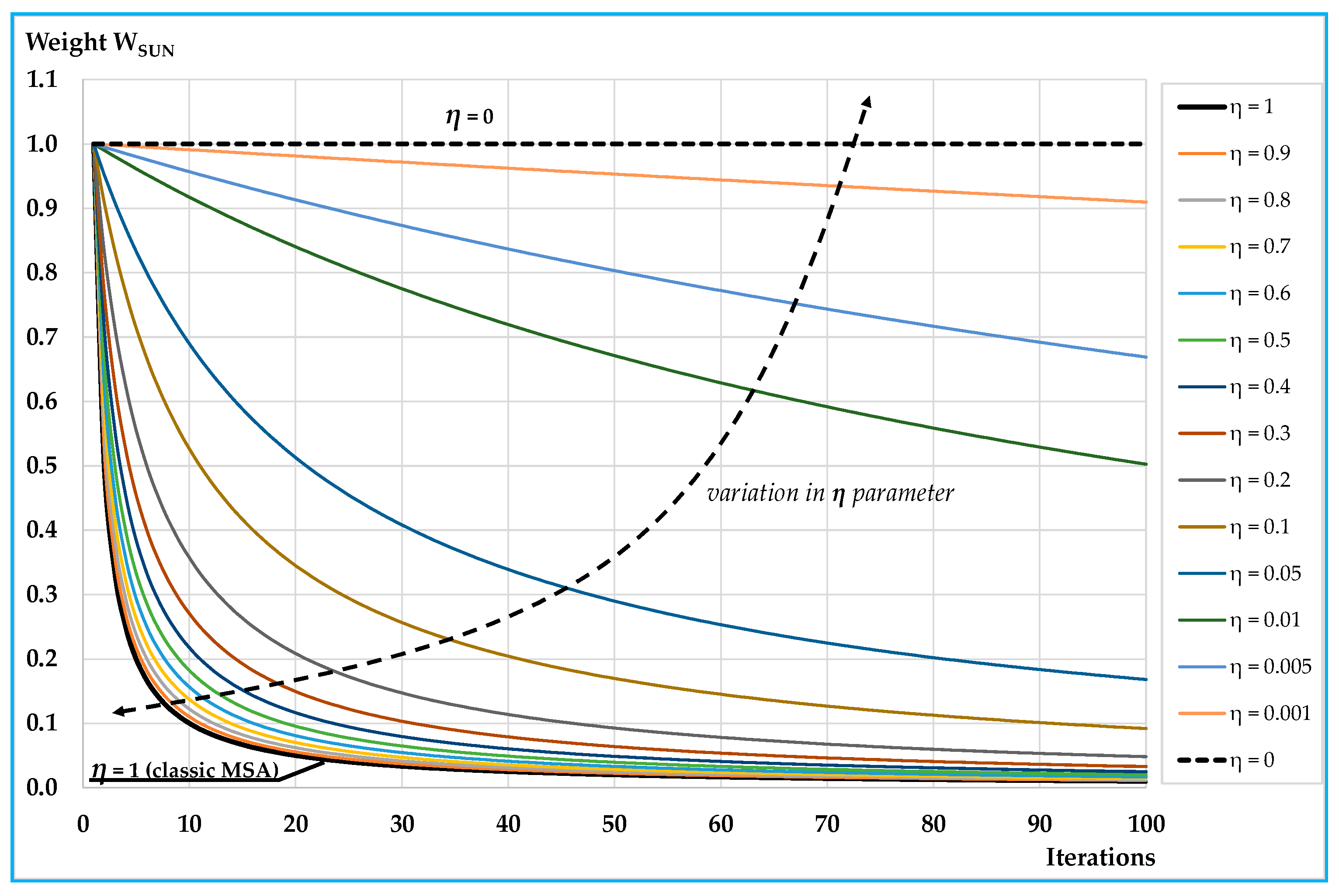
Since, as shown in Appendix B, most of the MSA-based algorithms proposed in the literature for solving the traffic assignment problem are based on a modification of the weight formulation (i.e., term 1/k in the traditional MSA algorithm), our proposal consists in providing a further variant of the MSA-FA algorithm substituting the term k in Equation (5) or (6) with the following function:

ξ(k) = 1 + (k–1) · η

(7)

where η is a parameter between 0 and 1; for η = 1 we obtain the classic MSA algorithm, and for η = 0 we obtain that f^k = f_SUN^k (in this case the algorithm does not consider at each iteration the results of the previous ones). This method tends to muffle the weight given to f ^k−1 (with η < 1) with respect to the corresponding weight given with the classic MSA algorithm. The weights of f ^k−1, w₋₁, and f_SUN^k, w_SUN, at each iteration k become:

w₋₁ = ((k–1) · η)/(1 + (k–1) · η)

(8)

w_SUN = 1/(1 + (k–1) · η)

(9)

In Algorithm 2 the code of the generalised MSA-FA algorithm (i.e., GMSA-FA) is reported. Figure 1 reports the values at each iteration k of w_SUN (equal to 1 − w₋₁) for values of η between 1 (classic MSA) and 0 and for the first 100 iterations.

Algorithm 2 Generalised MSA-FA algorithm

1:   k = 0 2:   f0 = 0 3:   do while |fSUNk − f k−1|/f k−1 ≥ ε 4:   k = k + 1 5:   ck = χ(f k−1) 6:   fSUNk = φSUN(ck) 7:   fk = f k−1 + 1/ξ(k) · (fSUNk − f k−1) 8:   loop 9:   f * = fk 10:   end

It can be noted that the weight of f_SUN^k decreases less rapidly for lower values of parameter η. Convergence of the proposed algorithm is stated in Appendix A, where the algorithm is shown to converge for each value of η > 0.

4. Numerical Results

Numerical tests were conducted on a small test network and on two real-scale networks (an urban and a rural network). Each network, by means of the graph theory, was represented as a set of links and nodes. The links represent the phases of the trips (as for instance, the roads) and the nodes represent the transitions between two consecutive links. Among the nodes, it is possible to identify the centroid nodes that represent the origin and destination of each trip.

4.1. Small Network

The small network consisted of 16 oriented links (see Figure 2), whose link performances (i.e., the link travel times) were expressed by means of a BPR function [26], that is:

t_l = (L_l/v_0,l) · (1 + α · (f_l/Cap_l)^β)

(10)

where t_l is the travel time associated to link l; L_l is the length of link l; v_o,l is the free-flow speed associated to link l; f_l is the link flow associated to link l; Cap_l is the capacity of link l; α and β are function parameters. The main features of the considered network are summarised in

Table 1. Features of the small network.

Link	Length (km)	Capacity (veh/h)	Free-Flow Speed (km/h)	BPR Param. α	BPR Param. β
1–5	2	1800	60	2.0	4.0
5–1	2	1800	60	2.0	4.0
1–3	2	1800	50	2.0	4.0
3–1	2	1800	50	2.0	4.0
3–6	3	3600	90	0.2	4.0
6–3	3	3600	90	0.2	4.0
5–6	2	3600	80	0.2	4.0
6–5	2	3600	80	0.2	4.0
5–2	4	1800	50	2.0	4.0
2–5	4	1800	50	2.0	4.0
6–2	5	1800	70	2.0	4.0
2–6	5	1800	70	2.0	4.0
6–4	5	3600	90	0.2	4.0
4–6	5	3600	90	0.2	4.0
4–2	3	1800	60	2.0	4.0
2–4	3	1800	60	2.0	4.0

.

Bold links have higher capacity and free-flow speed with respect to the others. We assume that nodes 1, 2, 3 and 4 are also the origins and destinations of the trips, according to the OD vector, d, reported in

Table 2. Origin-destination vector of the small network.

Origin	Destination	OD Flow (veh/h)
1	2	1700
2	1	600
1	3	500
3	1	700
1	4	650
4	1	100
2	3	800
3	2	450
2	4	750
4	2	450
3	4	1250
4	3	200

. In the tests, we adopted Multinomial Logit as the stochastic path choice model and assumed that the cost of each link was equal to the running time expressed in minutes with parameter θ equal to 0.5 (coefficient of variation about 0.2). We implemented the proposed algorithm in Visual Basic. We tested the proposed algorithm with the following values of parameter η: 1 (classic MSA), 0.9, 0.8, 0.7, 0.6, 0.5, 0.4, 0.3, 0.2, 0.1, 0.05, 0.01, 0. For each value, we tested the OD vector reported in Table 2 multiplied by the following coefficients: 0.6, 0.8, 1.0, 1.2, 1.4, 1.6, 1.8, and 2.0. The use of different OD vectors, as well as different multipliers, is to analyse the algorithm’s performance for different congestion levels. Indeed, the vectors thus obtained produce average saturation degrees (flow/capacity ratio) on the network between 0.249 and 0.838, as reported in

Table 3. Average saturation degrees on the small network.

Matrix	0.6 d	0.8 d	1.0 d	1.2 d	1.4 d	1.6 d	1.8 d	2.0 d
Av. Sat. Degree	0.249	0.332	0.415	0.499	0.583	0.668	0.753	0.838

. The convergence threshold was assumed to be equal to 1% for all tests.

In all cases, the proposed algorithm was able to reduce the iterations for the convergence with some values of η lower than 1 (MSA). It can be noted that, upon reducing the value of η, the number of iterations starts to decrease until a minimum value is reached. The number of iterations then begins to increase until the case of η = 0 when, according to also to the theoretical properties examined in Appendix A, the algorithm may not converge.

In

Table 4. Results on the small network.

	Iterations Needed for Convergence
Matrix	0.6 d	0.8 d	1.0 d	1.2 d	1.4 d	1.6 d	1.8 d	2.0 d
η = 1(MSA)	7	8	45	96	168	287	422	582
η = 0.9	6	7	40	80	147	239	350	478
η = 0.8	6	8	34	71	126	201	291	397
η = 0.7	5	11	30	63	107	170	247	329
η = 0.6	5	14	29	54	92	143	209	279
η = 0.5	4	15	27	48	81	125	183	243
η= 0.4	4	13	23	43	73	112	163	237
η = 0.3	5	11	24	46	81	133	208	310
η = 0.2	6	15	34	66	117	194	305	457
η = 0.1	8	26	61	123	222	374	591	892
η = 0.05	12	45	112	233	429	727	>999	>999
η = 0.01	31	182	504	>999	>999	>999	>999	>999
	Percentage Variations with Respect to MSA
Matrix	0.6 d	0.8 d	1.0 d	1.2 d	1.4 d	1.6 d	1.8 d	2.0 d
η = 1(MSA)	-	-	-	-	-	-	-	-
η = 0.9	−14%	−13%	−11%	−17%	−13%	−17%	−17%	−18%
η = 0.8	−14%	0%	−24%	−26%	−25%	−30%	−31%	−32%
η = 0.7	−29%	38%	−33%	−34%	−36%	−41%	−41%	−43%
η = 0.6	−29%	75%	−36%	−44%	−45%	−50%	−50%	−52%
η = 0.5	−43%	88%	−40%	−50%	−52%	−56%	−57%	−58%
η = 0.4	−43%	63%	−49%	−55%	−57%	−61%	−61%	−59%
η = 0.3	−29%	38%	−47%	−52%	−52%	−54%	−51%	−47%
η = 0.2	−14%	88%	−24%	−31%	−30%	−32%	−28%	−21%
η = 0.1	14%	225%	36%	28%	32%	30%	40%	53%
η = 0.05	71%	463%	149%	143%	155%	153%	-	-
η = 0.01	343%	2175%	1020%	-	-	-	-	-

In bold are reported the best results.

, the number of iterations required for convergence for all cases is reported (the algorithm was stopped in any event when the iterations reached 999); minimum values are written in bold. In the same table, the percentage variations in terms of iteration number are reported. However, it is worth noting that all variants of the algorithm provide the same results. The difference among them is only the number of iterations necessary to achieve the convergence condition. In Figure 3, the results of Table 4 are summarised.

Note that the reduction in the number of iterations, and hence, in computing time, provided by the proposed algorithm can be very significant for medium-high congested networks, i.e., up to −61% compared with the traditional version of the MSA algorithm.

4.2. Real-Scale Urban Network

The real-scale urban test network is the network of Benevento, a town in the south of Italy with about 61,000 inhabitants. The network, as represented in Figure 4, has 1577 oriented links, comprising about 216 km of roads, 678 nodes and 80 centroids (66 internal and 14 external). The peak-hour OD matrix was made available by studies carried out while drawing up the Urban Traffic Plan. The route choice model is Multinomial Logit with an implicit enumeration of paths according to the algorithm proposed in Reference [27].

In order to test the proposed algorithms under several network congestion levels, over the available OD matrix, seven other matrices were generated, multiplying all cells of the OD matrix by the following factors: 0.6, 0.8, 1.2, 1.4, 1.6, 1.8, and 2.0. The corresponding average saturation degrees are summarised in

Table 5. Average saturation degrees on the urban real-scale network.

Matrix	0.6 d	0.8 d	1.0 d	1.2 d	1.4 d	1.6 d	1.8 d	2.0 d
Av. Sat. Degree	0.246	0.324	0.400	0.472	0.545	0.618	0.691	0.764

.

On this network, we tested the proposed algorithm with the same values of parameter η as those adopted for the small test network; we tested the algorithm with two different values of the coefficient of variation (standard deviation to mean ratio), C_v, equal to 0.10 and 0.05. Moreover, in these cases, the proposed algorithm was able to reduce the iterations for convergence with some values of η lower than 1 (MSA). In this case, the best performances were obtained with values between 0.4 and 0.6 (see

Table 6. Results on the urban real-scale network (C_v = 0.10).

	Iterations Needed for Convergence
Matrix	0.6 d	0.8 d	1.0 d	1.2 d	1.4 d	1.6 d	1.8 d	2.0 d
η = 1(MSA)	5	8	17	32	50	52	55	61
η = 0.9	5	8	14	25	36	38	39	43
η = 0.8	5	8	12	19	27	28	28	32
η = 0.7	5	8	10	15	20	20	21	29
η = 0.6	5	7	9	12	15	15	20	26
η = 0.5	4	7	9	11	12	15	21	25
η = 0.4	4	7	10	11	12	18	24	27
η = 0.3	4	8	11	13	15	21	30	33
η = 0.2	4	10	14	17	20	28	41	45
η = 0.1	4	14	22	28	33	49	74	79
η = 0.05	4	22	37	48	58	88	136	146
η = 0.01	4	77	147	196	244	385	619	664
	Percentage Variations with Respect to MSA
Matrix	0.6 d	0.8 d	1.0 d	1.2 d	1.4 d	1.6 d	1.8 d	2.0 d
η = 1(MSA)	-	-	-	-	-	-	-	-
η = 0.9	0%	0%	−18%	−22%	−28%	−27%	−29%	−30%
η = 0.8	0%	0%	−29%	−41%	−46%	−46%	−49%	−48%
η = 0.7	0%	0%	−41%	−53%	−60%	−62%	−62%	−52%
η = 0.6	0%	−13%	−47%	−63%	−70%	−71%	−64%	−57%
η = 0.5	−20%	−13%	−47%	−66%	−76%	−71%	−62%	−59%
η = 0.4	−20%	−13%	−41%	−66%	−76%	−65%	−56%	−56%
η = 0.3	−20%	0%	−35%	−59%	−70%	−60%	−45%	−46%
η = 0.2	−20%	25%	−18%	−47%	−60%	−46%	−25%	−26%
η = 0.1	−20%	75%	29%	−13%	−34%	−6%	35%	30%
η = 0.05	−20%	175%	118%	50%	16%	69%	147%	139%
η = 0.01	0%	0%	−18%	−22%	−28%	−27%	−29%	−30%

In bold are reported the best results.

) for C_v = 0.10 and between 0.3 and 0.6 (see

Table 7. Results on the urban real-scale network (C_v = 0.05).

	Iterations Needed for Convergence
Matrix	0.6 d	0.8 d	1.0 d	1.2 d	1.4 d	1.6 d	1.8 d	2.0 d
η = 1(MSA)	5	8	20	47	49	49	53	59
η = 0.9	5	7	16	34	36	36	38	42
η = 0.8	4	7	13	25	26	26	34	38
η = 0.7	4	6	10	18	19	21	35	39
η = 0.6	4	6	9	14	14	20	31	34
η = 0.5	3	6	8	10	14	24	34	36
η = 0.4	3	5	9	10	16	27	40	43
η = 0.3	3	6	11	10	20	34	50	54
η = 0.2	3	8	14	12	27	46	71	76
η = 0.1	3	11	23	26	49	84	132	141
η = 0.05	4	17	39	45	90	158	251	269
η = 0.01	4	54	160	186	402	724	>999	>999
	Percentage Variations with Respect to MSA
Matrix	0.6 d	0.8 d	1.0 d	1.2 d	1.4 d	1.6 d	1.8 d	2.0 d
η = 1(MSA)	-	-	-	-	-	-	-	-
η = 0.9	0%	−13%	−20%	−28%	−27%	−27%	−28%	−29%
η = 0.8	−20%	−13%	−35%	−47%	−47%	−47%	−36%	−36%
η = 0.7	−20%	−25%	−50%	−62%	−61%	−57%	−34%	−34%
η = 0.6	−20%	−25%	−55%	−70%	−71%	−59%	−42%	−42%
η = 0.5	−40%	−25%	−60%	−79%	−71%	−51%	−36%	−39%
η = 0.4	−40%	−38%	−55%	−79%	−67%	−45%	−25%	−27%
η = 0.3	−40%	−25%	−45%	−79%	−59%	−31%	−6%	−8%
η = 0.2	−40%	0%	−30%	−74%	−45%	−6%	34%	29%
η = 0.1	−40%	38%	15%	−45%	0%	71%	149%	139%
η = 0.05	−20%	113%	95%	−4%	84%	222%	374%	356%
η = 0.01	−20%	575%	700%	296%	720%	1378%	-	-

In bold are reported the best results.

) for C_v = 0.05; the reductions in the number of iterations reached −76% (C_v = 0.10) and −79% (C_v = 0.05) with respect to the traditional version of the MSA algorithm. In Figure 5 and Figure 6, the results of Table 6 and Table 7 are illustrated. Moreover, in this case, the utility of the proposed algorithm is more significant for medium-high demand levels.

4.3. Real-Scale Rural Network

The real-scale rural test network is the regional road network of Campania, an Italian Region with more than 5.8 million inhabitants. The network, as represented in Figure 7, has 764 road links, representing about 8700 km of roads, 262 road nodes and 91 centroids.

We tested the proposed approach considering the OD matrix in the morning peak-hour, where the total trips are 165,328 veh/h; we also tested values of demand between 0.6 and 2.0 times the actual value, producing an average saturation degree between 0.4 and 1.25 (see

Table 8. Average saturation degrees on the rural real-scale network.

Matrix	0.6 d	0.8 d	1.0 d	1.2 d	1.4 d	1.6 d	1.8 d	2.0 d
Av. Sat. Degree	0.40	0.53	0.65	0.77	0.90	1.01	1.13	1.25

). Moreover, in this case, we use the Multinomial Logit route choice model with the implicit enumeration of paths [27].

On this network, we tested the proposed algorithm with the same values of parameter η previously adopted, assuming a coefficient of variation equal to 0.3. Moreover, in these cases, the proposed algorithm was able to reduce the iterations for convergence with some values of η lower than 1 (MSA). The best performances were obtained with values between 0.3 and 0.6 (see

Table 9. Results on the rural real-scale network.

	Iterations Needed for Convergence
Matrix	0.6 d	0.8 d	1.0 d	1.2 d	1.4 d	1.6 d	1.8 d	2.0 d
η = 1(MSA)	19	26	26	29	36	54	63	70
η = 0.9	16	32	20	22	27	38	46	51
η = 0.8	14	24	18	17	21	28	33	39
η = 0.7	12	19	13	14	17	23	26	30
η = 0.6	10	15	11	11	14	18	21	26
η = 0.5	9	12	10	11	14	17	22	26
η = 0.4	8	11	11	13	16	21	27	35
η = 0.3	7	10	12	15	19	26	34	44
η = 0.2	9	12	16	21	27	36	48	62
η = 0.1	13	19	26	35	47	63	87	115
η = 0.05	19	31	45	61	84	117	163	218
η = 0.01	60	114	>999	258	366	525	747	>999
	Percentage Variations with Respect to MSA
Matrix	0.6 d	0.8 d	1.0 d	1.2 d	1.4 d	1.6 d	1.8 d	2.0 d
η = 1(MSA)	-	-	-	-	-	-	-	-
η = 0.9	−16%	23%	−23%	−24%	−25%	−30%	−27%	−27%
η = 0.8	−26%	−8%	−31%	−41%	−42%	−48%	−48%	−44%
η = 0.7	−37%	−27%	−50%	−52%	−53%	−57%	−59%	−57%
η = 0.6	−47%	−42%	−58%	−62%	−61%	−67%	−67%	−63%
η = 0.5	−53%	−54%	−62%	−62%	−61%	−69%	−65%	−63%
η = 0.4	−58%	−58%	−58%	−55%	−56%	−61%	−57%	−50%
η = 0.3	−63%	−62%	−54%	−48%	−47%	−52%	−46%	−37%
η = 0.2	−53%	−54%	−38%	−28%	−25%	−33%	−24%	−11%
η = 0.1	−32%	−27%	0%	21%	31%	17%	38%	64%
η = 0.05	0%	19%	73%	110%	133%	117%	159%	211%
η = 0.01	216%	338%	-	790%	917%	872%	1086%	-

In bold are reported the best results.

); the reductions in the number of iterations reached −69% with respect to the traditional version of the MSA algorithm. In Figure 8, the results of Table 9 are illustrated.

4.4. Application to a Network Design Problem

The proposed algorithm was tested inside a procedure for solving Network Design Problem (NDP) on the rural real-scale network described in Section 4.3. In particular, we considered a network capacity expansion problem [28] where there were limited resources for improving the performances of a rural road network. In this problem, the current configuration of the road network is known, and no other roads can be added to it; instead, each existing road can be improved, increasing its capacity and free-flow speed. The decision variables of this problem are binary, y_i = 0/1, where y_i = 1 indicates that road i is improved in the solution, while y_i = 0 indicates that road i remains in the starting configuration. The details of NDP and of its model formulation are reported in Appendix C.

In order to compare the results obtained with the proposed muffled algorithm and the classic MSA, we tested the Neighbourhood Search Algorithm (NSA) with steepest descent method; it was used, for instance, in References [28,29]. A brief description of the algorithm is reported in Appendix D.

The tests were conducted under the actual demand (1.0 d), and therefore, assuming the parameter η = 0.5 in the muffled proposed algorithm, since it is the best value for this demand level (see Table 9). The results of the comparison between MSA and muffled algorithm are summarised in

Table 10. Comparison between algorithms.

	MSA (η = 1.0)	Muffled (η = 0.5)	% Difference
Examined solutions	6019	6223	3.39%
Examined neighbourhoods	59	61	3.39%
SNLs	72,893	39,103	−46.36%
Computing time [h]	5.83	3.25	−44.18%
Starting objective function value [€]	38,010,674,174	37,971,126,906
Final objective function value [€]	29,363,169,248	29,305,075,507
% variation of objective function value	−22.75%	−22.82%

; note that the computing time saved is about 44% (over 2.5 h). The different numbers of examined neighbourhoods and objective function values are only due to the convergence test; indeed, even if the convergence test is the same, the flows generated at each iteration of the algorithms can be slightly different and may influence the final solution. In Figure 9, the comparison among MSA and muffled algorithm is reported in terms of computing times and objective function values. These results underline the utility of the proposed algorithm inside Network Design Problem solution procedures; indeed, we have to consider also that several meta-heuristic algorithms use NSAs as subroutines (Scatter Search, Tabu Search, etc.), and then, the computing time saved should be multiplied by the number of NSAs performed for reaching the final solution.

5. Conclusions and Research Prospects

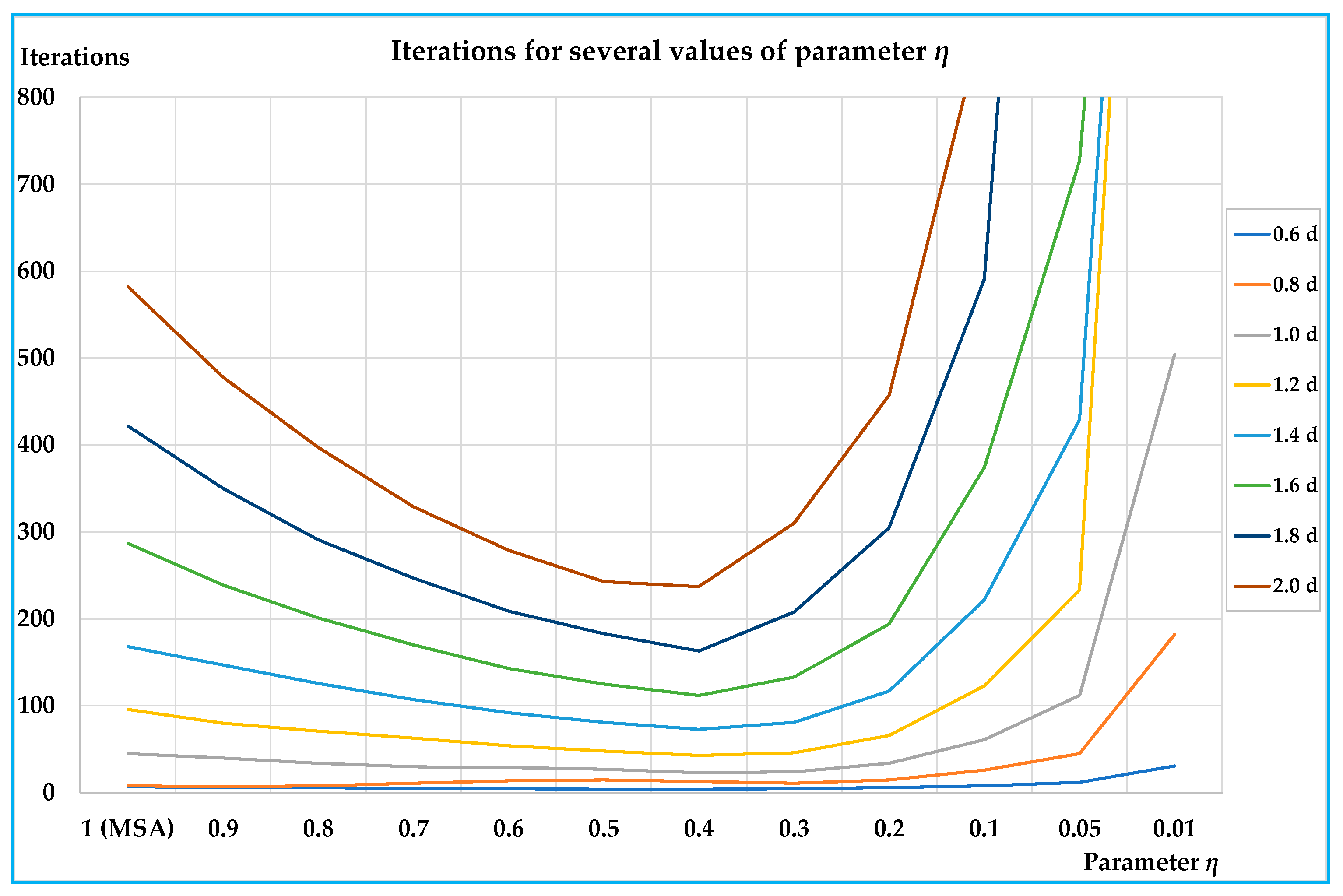
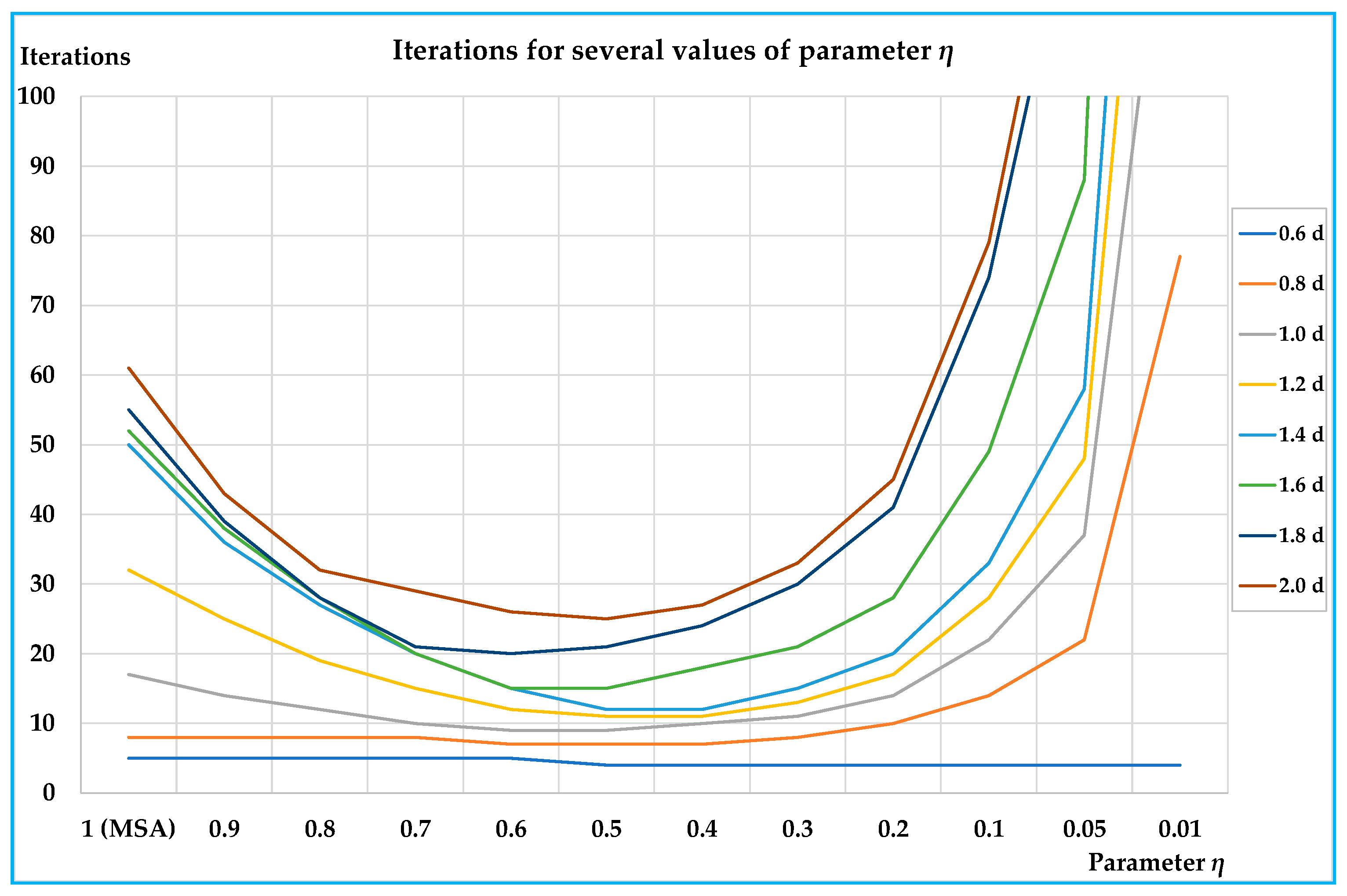
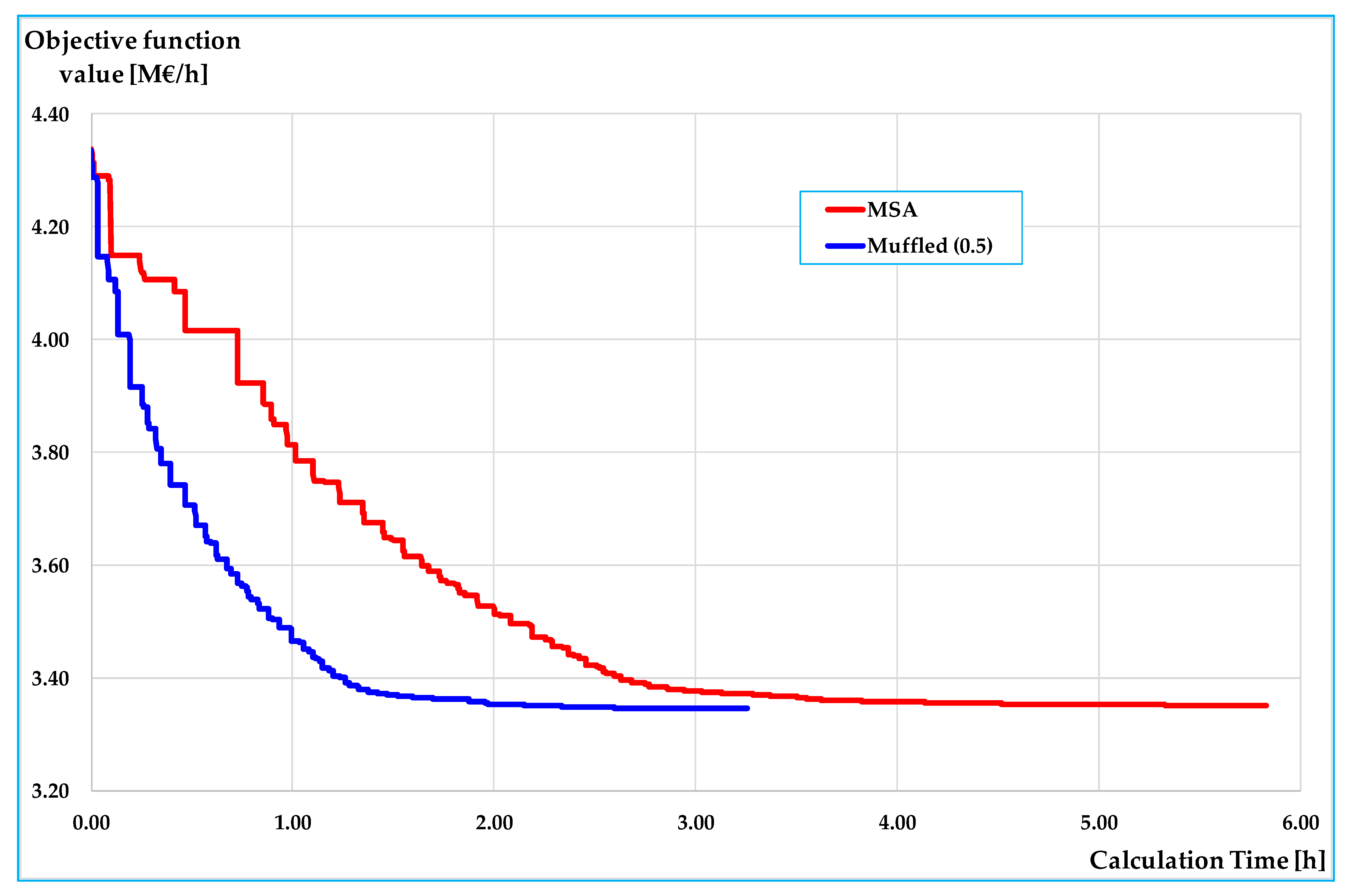
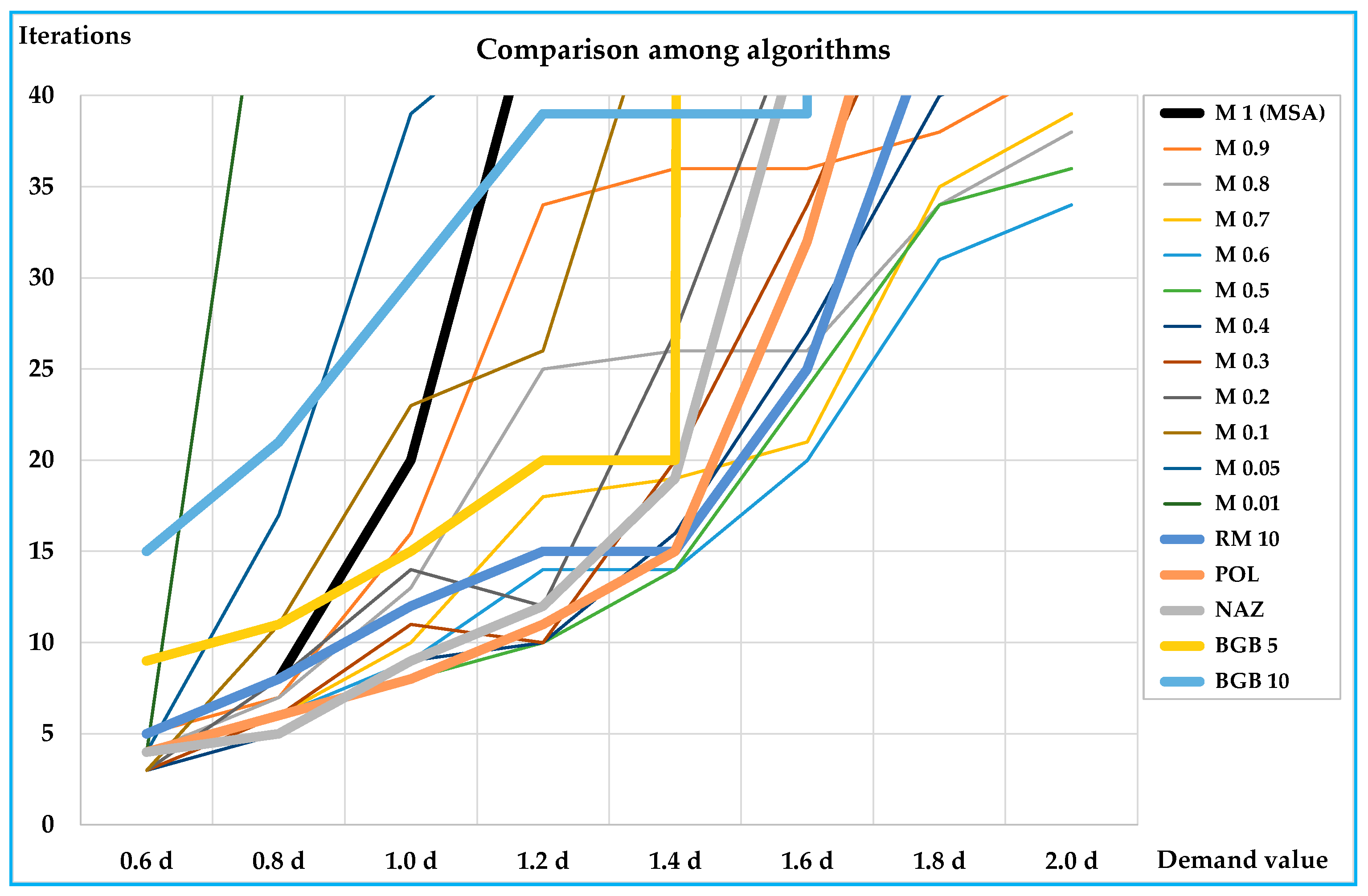
The results obtained on the small and on the real-scale networks show that the proposed algorithm is able to reduce the number of iterations for convergence, and hence, computing times compared with the classic MSA approach; in particular, the reductions arrive in percentage up to –79% with respect to the classic MSA for the best value of the parameter. On all networks the results are similar, showing that the benefits of the proposed algorithm are significant for medium-high congested demand levels (average saturation degrees over about 0.4); less significant, but not negligible, are the benefits for lower demand levels.

In all tests, the best values of parameter η lie between 0.3 and 0.6. An important characteristic of the proposed algorithm is that there is a parameter that can be opportunely chosen, so to optimise the performances before starting with network design procedure; moreover, examining Figure 3, Figure 5, Figure 6 and Figure 8 it is evident that, especially for medium-high levels of demand, a minimum can be found. In our test, we adopt a 0.1 step, but the parameter η can assume any value between 1 (MSA) and 0 (0 excluded), and therefore, other values can be tested in order to find the one that minimises the computing times.

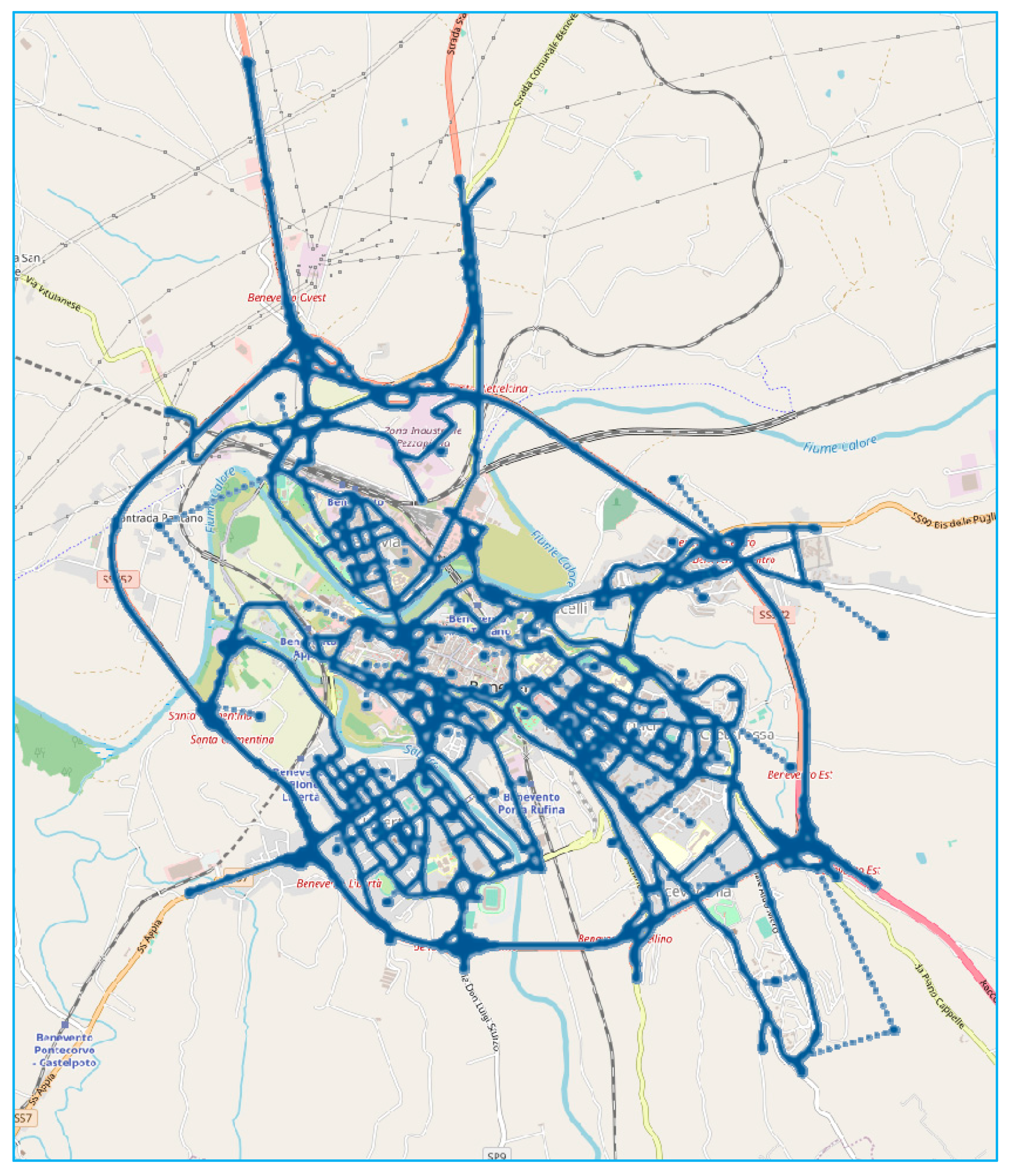
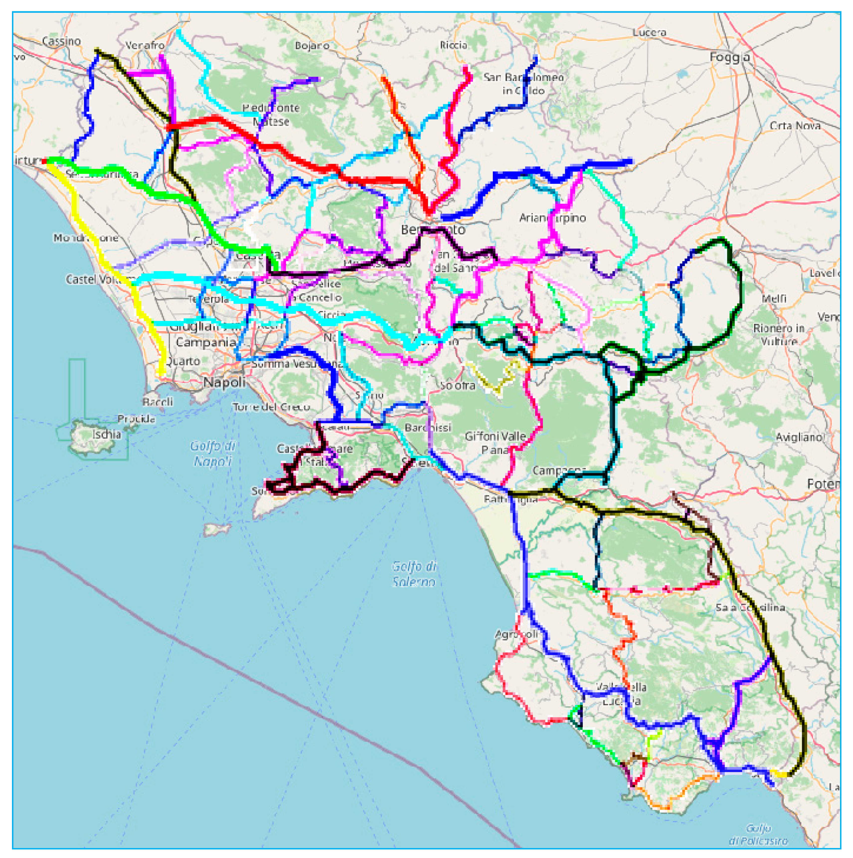
The reduction in computing times can be not important if the assignment procedure is performed only once or a few times: with current computing capabilities, the savings are lower than a minute on the real-scale network. By contrast, if the assignment is a subroutine of the Network Design Problem, that requires the calculation of the equilibrium traffic flows many thousands of times, the reduction in computing time of an assignment is transferred to the computing time of the network design algorithm, allowing as much as several days to be saved in the calculation. In our test on the rural road network, the proposed algorithm is able to save about 44% of computing time, equivalent to about 2.5 h for a single NSA procedure.

Future research will focus on testing other real-scale networks, testing the algorithm on multimodal networks and under the assumption of elastic demand and proposing a similar algorithm for solving the combined assignment-control problem. Moreover, testing the proposed algorithm within other real-scale network design procedures will be the subject of future studies.

References

1. Wardrop, J.G. Some theoretical aspects of road traffic research. Proc. Inst. Civ. Eng. Part II 1952, 1, 325–378. [Google Scholar] [CrossRef]
2. Sheffi, Y.; Powell, W.B. A comparison of stochastic and deterministic traffic assignment over congested networks. Transp. Res. Part B Methodol. 1981, 15, 53–64. [Google Scholar] [CrossRef]
3. Sheffi, Y.; Powell, W.B. An algorithm for the equilibrium assignment problem with random link times. Networks 1982, 12, 191–207. [Google Scholar] [CrossRef]
4. Powell, W.B.; Sheffi, Y. The convergence of equilibrium algorithms with predetermined step sizes. Transp. Sci. 1982, 6, 45–55. [Google Scholar] [CrossRef]
5. Cantarella, G.E. A general fixed-point approach to multimodal multi-user equilibrium assignment with elastic demand. Transp. Sci. 1997, 31, 107–128. [Google Scholar] [CrossRef]
6. D’Acierno, L.; Montella, B.; De Lucia, F. A stochastic traffic assignment algorithm based on Ant Colony Optimisation. Lect. Notes Comput. Sci. 2006, 4150, 25–36. [Google Scholar]
7. Cantarella, G.E.; de Luca, S.; Di Gangi, M.; Di Pace, R. Stochastic equilibrium assignment with variable demand: Literature review, comparisons and research needs. WIT Trans. Built Environ. 2013, 130, 349–364. [Google Scholar]
8. Cantarella, G.E.; Cartenì, A.; de Luca, S. Stochastic equilibrium assignment with variable demand: Theoretical and implementation issues. Eur. J. Oper. Res. 2015, 241, 330–347. [Google Scholar] [CrossRef]
9. Polyak, B.T. New method of stochastic approximation type. Automat. Rem. Contr. 1990, 51, 937–946. [Google Scholar]
10. Nagurney, A.; Zhang, D. Projected Dynamical Systems and Variational Inequalities with Applications; Kluwer: Boston, MA, USA, 1996. [Google Scholar]
11. Bar-Gera, H.; Boyce, D. Solving a non-convex combined travel forecasting model by the method of successive averages with constant step sizes. Transp. Res. Part B Methodol. 2006, 40, 351–367. [Google Scholar] [CrossRef]
12. Cantarella, G.E.; De Luca, S.; Di Gangi, M.; Di Pace, R. Approaches for solving the stochastic equilibrium assignment with variable demand: Internal vs. external solution algorithms. Optim. Methods Softw. 2015, 30, 338–364. [Google Scholar] [CrossRef]
13. Liu, H.X.; He, X.; He, B. Method of Successive Weighted Averages (MSWA) and self-regulated averaging schemes for solving stochastic user equilibrium problem. Netw. Spat. Econ. 2009, 9, 485–503. [Google Scholar] [CrossRef]
14. Di Gangi, M.; Cantarella, G.E.; Vitetta, A. Solving stochastic frequency-based assignment to transit networks with pre-trip/en-route path choice. EURO J. Transp. Logist. 2019, 8, 661–681. [Google Scholar] [CrossRef]
15. Cantarella, G.E.; Di Febbraro, A.; Di Gangi, M.; Giannattasio, O. Solving stochastic assignment to transportation networks with TVs and AVs. Transp. Res. Procedia 2020, 42, 7–18. [Google Scholar] [CrossRef]
16. Cantarella, G.E.; Di Febbraro, A. Transportation Systems with Autonomous Vehicles: Models and algorithms for equilibrium assignment. Transp. Res. Procedia 2017, 27, 349–356. [Google Scholar] [CrossRef]
17. Mokkadem, A.; Pelletier, M. A generalization of the averaging procedure: The use of two-time-scale algorithms. SIAM J. Control. Optim. 2011, 49, 1523–1543. [Google Scholar] [CrossRef]
18. Cascetta, E.; Gallo, M.; Montella, B. Models and algorithms for the optimization of signal settings on urban networks with stochastic assignment. Ann. Oper. Res. 2006, 144, 301–328. [Google Scholar] [CrossRef]
19. Magnanti, T.; Wong, R. Network design and transportation planning: Models and algorithms. Transp. Sci. 1984, 18, 181–197. [Google Scholar] [CrossRef] [Green Version]
20. Yang, H.; Bell, M.G.H. Models and algorithms for Road Network Design: A review and some new developments. Transp. Rev. 1998, 18, 257–278. [Google Scholar] [CrossRef]
21. Feremans, C.; Labbé, M.; Laporte, G. Generalized network design problems. Eur. J. Oper. Res. 2003, 148, 1–13. [Google Scholar] [CrossRef]
22. Farahani, R.Z.; Miandoabchi, E.; Szeto, W.Y.; Rashidi, H. A review of urban transportation network design problems. Eur. J. Oper. Res. 2013, 229, 281–302. [Google Scholar] [CrossRef] [Green Version]
23. Zilioniene, D.; D’Acierno, L.; Botte, M.; Gallo, M. A general methodology for reducing computing times of road network design algorithms. Int. J. Supply Oper. Manag. 2019, 6, 126–141. [Google Scholar]
24. Cascetta, E. Transportation Systems Analysis: Models and Applications; Springer: New York, NY, USA, 2009. [Google Scholar]
25. Cantarella, G.E.; Watling, D.; de Luca, S.; Di Pace, R. Dynamics and Stochasticity in Transportation Systems: Tools for Transportation Network Modeling; Elsevier: Amsterdam, The Netherlands, 2019. [Google Scholar]
26. Bureau of Public Roads. Traffic Assignment Manual; U.S. Department of Commerce, Urban Planning Division: Washington, DC, USA, 1964.
27. Dial, R.B. A probabilistic multi-path traffic assignment model which obviates path enumeration. Transp. Res. 1971, 5, 83–111. [Google Scholar] [CrossRef]
28. Gallo, M.; D’Acierno, L.; Montella, B. A meta-heuristic algorithm for solving the road network design problem in regional contexts. Procedia Soc. Behav. Sci. 2012, 54, 84–95. [Google Scholar] [CrossRef] [Green Version]
29. Gallo, M.; D’Acierno, L.; Montella, B. A meta-heuristic approach for solving the Urban Network Design Problem. Eur. J. Oper. Res. 2010, 201, 144–157. [Google Scholar] [CrossRef]
30. Blum, J.R. Multidimensional stochastic approximation methods. Ann. Math. Stat. 1954, 25, 737–744. [Google Scholar] [CrossRef]
Figure 1. Values of weights wSUN.
Applsci 10 05698 g001
Figure 2. Small network.
Applsci 10 05698 g002
Figure 3. Results on the small network.
Applsci 10 05698 g003
Figure 4. Urban real-scale network.
Applsci 10 05698 g004
Figure 5. Results on the urban real-scale network (Cv = 0.10).
Applsci 10 05698 g005
Figure 6. Results on the urban real-scale network (Cv = 0.05).
Applsci 10 05698 g006
Figure 7. Rural real-scale network.
Applsci 10 05698 g007
Figure 8. Results on the rural real-scale network.
Applsci 10 05698 g008
Figure 9. Comparison between algorithms in terms of computing times vs. objective function values.
Applsci 10 05698 g009