Adaptive Trajectory Tracking Safety Control of Air Cushion Vehicle with Unknown Input Effective Parameters

Abstract

This paper studies the trajectory tracking control problem of an Air Cushion Vehicle (ACV) with yaw rate error constraint, input effective parameters, model uncertainties and external wind disturbance. Firstly, based on the four-degree of freedom (DOF) vector mathematical mode of ACV, the radial basis function neural network (RBFNN) is adopted to provide the estimation of model uncertainties and external wind disturbance. Then, an adaptive Nussbaum gain-based approach is incorporated with the backstepping control scheme to handle the unknown input efficient parameters. To avoid the complicated derivative of the virtual control laws, the command filter and auxiliary systems are introduced in backstepping. Furthermore, combing a barrier Lyapunov function (BLF) with backstepping technique, a novel trajectory tracking safety controller is designed to ensure all signals of the closed-loop system are uniformly ultimately bounded, while the yaw rate error is within the pre-set safe range. Finally, the simulation results show the effectiveness of the controller scheme.

1. Introduction

An air-cushion vehicle (ACV), which is a high-performance ship, has a flexible skirt system at the bottom and can be lifted by an air cushion force. Compared with traditional marine surface vessels, its unique design makes it perform better at high speeds with a high wave resistance, strong flexibility and amphibious performance. Therefore, the ACV is used in marine transportation [1], military, rescue mission [2], scientific and marine development projects [3].

The ACV can easily exhibit stalling, sideslip, tail swing, roll and drift phenomena during turning at high speeds; thus, high-precision control and partial state safety constraints are necessary to avoid these phenomena. An accurate mathematical model is the basis for realizing safety and precision control.

From a review of the available literature about the ACV, only mathematical models with three DOFs were adopted [4,5,6,7,8,9,10]. However, the roll angle has a substantial influence on the turning radius of the ACV. In addition, the roll angle is also an important safety indicator. In actual sailing, the roll angle must be determined within a certain range; otherwise, the ship deck will enter the water and cause the ship to overturn. Four DOFs models, including surge, sway, roll and yaw motion, are established in these papers [11,12]. It is also shown that the four DOFs model is more suitable for engineering applications than the three DOFs model. In these articles, the idea of separation modelling is used. The forces and moments including hydrodynamics, aerodynamics, air momentum, air propeller forces, rudder forces and skirt drag are represented in the four DOFs. However, there is far less research literature on hovercrafts than on ordinary surface vessels [13]. If the model of the ACV is transformed into a vector form similar to the ordinary surface ship, not only can the differences between them be compared, but this can also facilitate the promotion and application of the latter in the former.

The safe control of the ACV can also be understood as the constraint problem of some state variables during high-speed sailing. The preset performance function method, model predictive control approach, barrier Lyapunov functions, reference setting method and control skill based on invariant settings or permissible settings are typical techniques for solving constraint problems [14,15,16,17,18,19]. A preset performance path tracking controller for under-actuated surface ships with input saturation and external disturbances was proposed to assure that the positional errors were limited to a predetermined range [20]. For a class of strict feedback nonlinear systems [21], a backstepping controller was proposed based on the preset performance, taking into account both the steady-state and temporary state performance. In [22], surface ships with full-state constraints and dynamic uncertainties were controlled based on the barrier Lyapunov function, which was used to prevent state violation constraints. For the longitudinal model of the hypersonic vehicle, the adaptive neural control method was designed by using a neural network to constrain the angle of attack within the specified safety range [23]. In [24], the author proposed Lyapunov functions to solve the problem of trajectory tracking control of fully actuated unmanned vessels with input and output asymmetric constraints. An adaptive neural network tracking controller that combined the backstepping method, adaptive neural network and preset performance was designed to approximate unmoulded dynamics and external disturbances [25]. For the ACV, when it turns at high speeds, the yaw rate changes too much, which will cause side-slip. At the same time, the comfort of the driver will also be affected. Therefore, this paper, is the first to combine the BLF, Nussbaum function and backstepping methods to address the rudder nonlinearity and constraints of the yaw rate error.

In engineering applications, we need to convert the control force and moment into the pitch angle of the air duct propeller and rudder angle of the air rudder to control the ACV, respectively. Unfortunately, very few studies are available in this regard. An adaptive terminal sliding model control scheme is proposed to address the servo system uncertainties in dynamic positioning [26]. In 1983, Nussbaum R D proposed Nussbaum functions to solve the system control coefficient uncertainty and model parameter uncertainty [27]. A robust Nussbaum gain-based approach is designed for adaptive fuzzy asymptotic control of multiple input and multiple output nonlinear systems [28]. Then, in [29], the author studied the application of Nussbaum functions in system stabilization. The unknown control direction is resolved effectively by the Nussbaum gain function, and the boundedness of uncertain time-varying parameters is guaranteed by using the continuous projection algorithm [24]. The Nussbaum analysis tool was adopted to study the motion control problem of robotic systems with the generalized actuator [30]. To the best of our knowledge, this study is the first to introduce the Nussbaum function into the study of ACV to solve the problem of actuator effective input parameters.

Motivated by the above analyses, a novel control method is designed to solve the trajectory tracking of ACVs under the consideration of unknown effective input parameters, the turning rate error within the safety limit and wind disturbance. The main contributions of this paper are expressed as follows:

• A four-DOF vector mathematical model of an ACV is proposed to simplify the controller design. Based on the vector model, RBFNN is adopted to provide the estimation of the model uncertainties and external wind disturbance. Command filters and auxiliary systems are integrated with the control law such that the complicated computation of the virtual control derivative can be avoided.
• A Nussbaum function is first introduced into the study on the ACV to solve the unknown nonlinear relationships between the actuator’s input and output.
• The yaw rate error constraint of the ACV is approached by introducing a BLF in combination with an adaptive Nussbaum function to prevent the tail swing phenomenon caused by the large yaw rate.
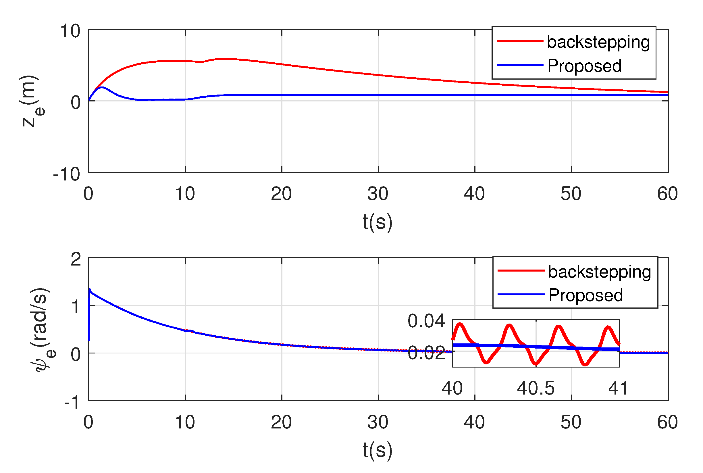
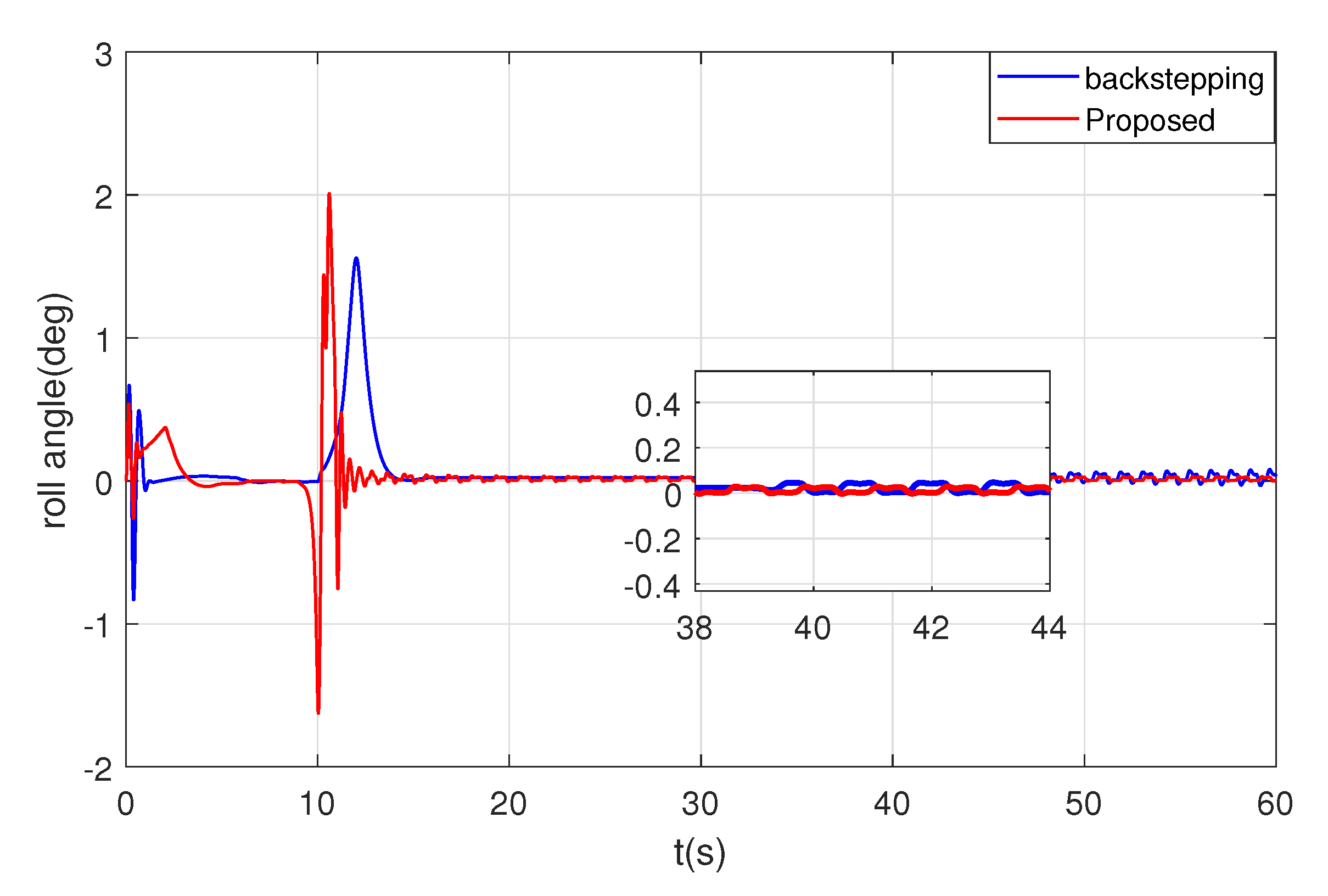
• The stability analysis shows that the proposed control algorithm can accurately track the set trajectory and ensure that the yaw rate error and the roll angle are within a safe range. All the error signals of the whole closed-loop control system can converge into a small neighbourhood around zero. The comparative simulation results illustrate the effectiveness and superiority of the proposed trajectory tracking control scheme.

The rest of the paper is organized as follows. In Section 2, the preliminaries and a mathematical model are provided. The trajectory tracking controller is designed in Section 3. Numerical simulation results are drawn in Section 4. Finally, Section 5 summarizes the conclusion.

2. System Description and Analysis

2.1. Preliminaries

Lemma 1

([12]). For an unknown continuous nonlinear function $f\left(x\right):R^n\to R$, the RBFNN can be used to approximate it over a compact set $\Omega \subseteq R^m$ as follows:

$$f\left(x\right)=W^{*T}H\left(x\right)+\epsilon \left(x\right).$$

(1)

where $x\in R^n$ is the input vector, $H\left(x\right)={\left[h_1\left(x\right),\cdots h_m\left(x\right)\right]}^T$ is the radial basis function vector and $h_j=exp(-\frac{{∥\mathbf{x}-c_j∥}^2}{2b_j^2})$. $c={\left[c_{ij}\right]}_{n\times m}$ is the center and $b_j$ is the width of the neural cell of the hidden layer. $\epsilon \left(x\right)$ denotes the approximate error satisfying $\epsilon \left(x\right)\le \overline{\epsilon },\overline{\epsilon }$ is an arbitrary small positive constant. The RBF optimal weight vector is $W^{*}={\left[w_1^{*},···,w_m^{*}\right]}^T$. The weight vector of $W^{*}$ is calculated by:

$$W^{*}=arg\underset{\widehat{W}}{min}\{\underset{x\in \Omega }{sup}|f\left(x\right)-{\widehat{W}}^{T}H\left(x\right)|\},$$

where $\widehat{W}$ is the estimate value of $W^{*}$, which is produced by an adaptive update law.

Definition 1

([30]). If a function N(s) has the following properties, it is called a Nussbaum-type function:

$$\begin{array}{cc}\hfill \underset{k\to \pm \infty }{lim\; sup}\frac{1}{k}{\int }_0^{k}N\left(s\right)ds& =\infty \hfill \\ \hfill \underset{k\to \pm \infty }{lim\; inf}\frac{1}{k}{\int }_0^{k}N\left(s\right)ds& =-\infty \hfill \end{array}$$

(2)

Lemma 2

([30]). Suppose that $g_k\left(t\right)$ is an unknown time-varying function, which satisfies $g_k\left(t\right)\in \nabla =[g^{-},g^{+}]$ with $0\in \nabla$, $g^{-}={min}_{1\le k\le n\left(g_k\right)}$, and $g^{+}={max}_{1\le k\le n\left(g_k\right)}$. All $g_k$ have the same sign for $k=1,2,\dots ,n$. Let $V_g(t_0,t)$, $s_k\left(t\right)$ be smooth functions defined on $[t_0,t_f]$ with $V(t_0,t_f)$ being nonnegative, $s_k\left(t_0\right)$ being bounded, and $N\left(s_k\left(t\right)\right)$ being the Nussbaum gain defined in Definition 1. If the following inequality holds:

$$\begin{array}{cc}\hfill V(t_0,t)\le & \sum _{k=1}^n{e}^{-{\alpha }_{k}t}{\int }_{t_0}^t{g}_k\left(t\right)N\left({\zeta }_k\left(\lambda \right)\right){\dot{\zeta }}_k\left(\lambda \right)d\lambda +\sum _{k=1}^n{e}^{-{\alpha }_{k}t}{\int }_{t_0}^t{\int }_{t_0}^t{\dot{\zeta }}_k\left(\lambda \right)e^{{\alpha }_k\lambda }d\lambda +o,\hfill \end{array}$$

(3)

where ${\alpha }_k$ is a positive constant and o is a bounded variable, then the conclusion is drawn that $N\left({\zeta }_k\left(t\right)\right)$, $V(t_0,t_f)$, $e^{-{\alpha }_{k}t}{\int }_{t_0}^{t_f}{\dot{\zeta }}_k\left(\lambda \right)e^{{\alpha }_k\lambda }d\lambda$, $e^{-{\alpha }_{k}t}{\int }_{t_0}^{t_f}{g}_k\left(t\right)N\left({\zeta }_k\left(\lambda \right)\right){\dot{\zeta }}_k\left(\lambda \right)e^{{\alpha }_k\lambda }d\lambda$ must be bounded on the interval $[t_0,t_f]$ for $k=1,2,\dots ,n$.

Lemma 3

([31]). For any constant $x\in R$, if $\left|x\right|<k$, k is a constant, the following inequality holds:

$$\begin{array}{c}\hfill ln\frac{k^2}{k^2-x^2}\le \frac{x^2}{k^2-x^2}\end{array}$$

(4)

2.2. ACV Model

In this section, based on two reference frames, the earth coordinate system frame $O_E{X}_E{Y}_E{Z}_E$ and the body coordinate system frame $o_B{x}_B{y}_B{z}_B$, are shown in Figure 1. $X_E$ points north, $Y_E$ points east, $Z_E$ points into the earth. The origin $o_B$ is assumed to be located in the vessel center of mass. The $x_B$ points from aft to fore, $y_B$ points to right starboard. $z_B$ points to the bottom of the ship.

The four-degree of freedom kinetic equations of an air cushion vehicle is:

$$\begin{array}{c}\hfill m(\dot{u}-vr)=X\\ \hfill m(\dot{v}+ur)=Y\\ \hfill I_x\dot{p}=K\\ \hfill I_z\dot{r}=N\\ \hfill \end{array}$$

(5)

where m is the Mass of ACV, $I_x$ and $I_z$ are the moment inertia of x-axis and z-axis around the body coordinate system, $u,v,p,r$ are the surge velocity, the sway velocity, the roll angular velocity and the yaw rate of the ship, respectively. Then vector form of (4) is written as:

$$\begin{array}{c}\hfill {\mathit{M}}_{\mathit{H}}\dot{\mathbf{\nu }}+\mathit{C}\left(\mathbf{\nu }\right)\mathbf{\nu }=\mathbf{\tau }\end{array}$$

(6)

where ${\mathit{M}}_{\mathit{H}}$ denotes ACV’s hull inertia matrix. $\mathbf{\nu }={[u,v,p,r]}^T$ is the velocity vector in the body-fixed frame. $\mathit{C}\left(\mathbf{\nu }\right)$ denotes the skew-symmetric Coriolis. $\mathbf{\tau }={[X,Y,K,N]}^T$ denotes the forces and moments. They are given as:

$$\begin{array}{c}\hfill {\mathit{M}}_{\mathit{H}}=\left[\begin{array}{cccc}m\hfill & 0& 0& 0\\ 0\hfill & m& 0& 0\\ 0\hfill & 0& I_x& 0\\ 0\hfill & 0& 0& I_z\end{array}\right]\mathit{C}\left(\mathbf{\nu }\right)=\left[\begin{array}{cccc}0\hfill & 0& 0& -mv\\ 0\hfill & 0& 0& mu\\ 0\hfill & 0& 0& 0\\ 0\hfill & 0& 0& 0\end{array}\right]\end{array}$$

According to the idea of separate modelling, the forces and moments are specifically expressed as:

$$\begin{array}{cc}\hfill X& =X_a+X_h+X_m+X_p\hfill \\ \hfill Y& =Y_a+Y_h+Y_m\hfill \\ \hfill K& =K_a+K_h+K_m+K_{res}\hfill \\ \hfill N& =N_a+N_h+N_m+N_r\hfill \end{array}$$

(7)

where ${(·)}_h,{(·)}_a,{(·)}_m$ are hydrodynamics, aerodynamics, and air momentum, respectively. $X_p,N_r$ are the force and moment generated by air propeller and air rudder. $K_{grav}$ is roll recovery moment. Then, we conduct specific analysis.

2.2.1. Hydrodynamics

Hydrodynamics function is given as:

$$\begin{array}{c}\hfill {\mathbf{\tau }}_{\mathit{h}}={[X_h,Y_h,K_h,N_h]}^T\end{array}$$

(8)

and $X_h,Y_h,K_h,N_h$ denote the projection of hydrodynamics in four DOF. They are:

$$\begin{array}{cc}\hfill X_h& =X_{drag}\hfill \\ \hfill Y_h& =Y_{drag}+Y_{r}r+Y_{\dot{r}}\dot{r}+Y_{\left|r\right|r}\left|r\right|r+Y_{\left|v\right|r}\left|v\right|r+Y_{\dot{v}}\dot{v}\hfill \\ \hfill K_h& =K_{drag}+K_{r}r+K_{\dot{r}}\dot{r}+K_{\left|r\right|r}\left|r\right|r+K_{\left|v\right|r}\left|v\right|r+K_{\dot{v}}\dot{v}\hfill \\ \hfill N_h& =N_{drag}+N_{r}r+N_{\dot{r}}\dot{r}+N_{\left|r\right|r}\left|r\right|r+N_{\left|v\right|r}\left|v\right|r+N_{\dot{v}}\dot{v}\hfill \end{array}$$

where ${(·)}_{drag}$ are ship model hydrodynamic. $Y_{\dot{v}}$, $K_{\dot{v}}$, $N_{\dot{v}}$, $Y_r$, $K_r$, $N_r$, $Y_{\dot{r}}$, $K_{\dot{r}}$, $N_{\dot{r}}$, $Y_{\left|v\right|r}$, $K_{\left|v\right|r}$, $N_{\left|v\right|r}$, $Y_{\left|r\right|r}$, $K_{\left|r\right|r}$ and $N_{\left|r\right|r}$ are hydrodynamic coefficients.

$$\begin{array}{c}\hfill \left[\begin{array}{c}{X}_{drag}\\ Y_{drag}\\ K_{drag}\\ N_{drag}\end{array}\right]=\left[\begin{array}{c}\frac{1}{2}{C}_{xh}{\rho }_h{U}^2{L}_a^2\\ \frac{1}{2}{C}_{yh}{\rho }_h{U}^2{L}_a^2\\ \frac{1}{2}{C}_{kh}{\rho }_h{U}^2{L}_a^2\\ \frac{1}{2}{C}_{nh}{\rho }_h{U}^2{L}_a^2\end{array}\right]\end{array}$$

where $U=\sqrt{u^2+v^2}$ is the velocity of ACV, $C_{xh},C_{yh},C_{kh},C_{nh}$ are the hydrodynamic dimensionless coefficients, ${\rho }_h$ is the water density, $L_a$ is the cushion length.

Then we can get the hydrodynamic vector variable:

$$\begin{array}{c}\hfill {\mathbf{\tau }}_{\mathit{h}}={\mathit{M}}_{\mathit{h}}\dot{\mathbf{\nu }}+{\mathit{D}}_{\mathit{h}}\mathbf{\nu }+{\mathit{D}}_{\mathit{nh}}\left(\mathbf{\nu }\right)\mathbf{\nu }\end{array}$$

(9)

where ${\mathit{M}}_{\mathit{h}}$ is called the added mass and ${\mathit{D}}_{\mathit{h}}$ is a constant coefficient matrix that represents hydrodynamic damping. ${\mathit{D}}_{\mathbf{nh}}\left(\mathbf{\nu }\right)$ is also an equstion of hydrodynamic damping, but it is associated with the ship speed $\mathbf{\nu }$. They are given as follows:

$$\begin{array}{c}\hfill {\mathit{M}}_{\mathit{h}}=\left[\begin{array}{cccc}0\hfill & 0& 0& 0\\ 0\hfill & Y_{\dot{\nu }}& 0& Y_{\dot{r}}\\ 0\hfill & K_{\dot{\nu }}& 0& K_{\dot{r}}\\ 0\hfill & N_{\dot{\nu }}& 0& N_{\dot{r}}\end{array}\right]{\mathit{D}}_{\mathit{h}}=\left[\begin{array}{cccc}0\hfill & 0& 0& 0\\ 0\hfill & 0& 0& Y_r\\ 0\hfill & 0& 0& K_r\\ 0\hfill & 0& 0& N_r\end{array}\right]\end{array}$$

$$\begin{array}{c}\hfill {\mathit{D}}_{\mathit{nh}}\left(\mathbf{\nu }\right)=\left[\begin{array}{cccc}{\mu }_{x}u\hfill & {\mu }_{x}v& 0& 0\\ {\mu }_{y}u\hfill & {\mu }_{y}v& 0& Y_{\left|v\right|r}\left|v\right|+Y_{\left|r\right|r}\left|v\right|\\ {\mu }_{k}u\hfill & {\mu }_{k}v& 0& K_{\left|v\right|r}\left|v\right|+K_{\left|r\right|r}\left|v\right|\\ {\mu }_{n}u\hfill & {\mu }_{n}v& 0& N_{\left|v\right|r}\left|v\right|+N_{\left|r\right|r}\left|v\right|\end{array}\right]\end{array}$$

where

$$\begin{array}{c}\hfill {\mu }_x=\frac{1}{2}{C}_{xh}{\rho }_h{L}_a^2,{\mu }_y=\frac{1}{2}{C}_{yh}{\rho }_h{L}_a^2\\ \hfill {\mu }_k=\frac{1}{2}{C}_{kh}{\rho }_h{L}_a^2,{\mu }_n=\frac{1}{2}{C}_{nh}{\rho }_h{L}_a^2\end{array}$$

2.2.2. Aerodynamics

We assume that the point of action of the aerodynamics forces on the ship is $(x_a,y_a,z_a)$. Aerodynamics forces and moments vector variable is:

$$\begin{array}{c}\hfill {\mathbf{\tau }}_{\mathbf{a}}=[X_a,Y_a,K_a,N_a]\end{array}$$

(10)

$X_a,Y_a,K_a,and{N}_a$ denote the projection of aerodynamics in four DOF. They are:

$$\begin{array}{cc}\hfill X_a& =-\frac{1}{2}{\rho }_a{V}_a^2{C}_{xa}{S}_a\hfill \\ \hfill Y_a& =\frac{1}{2}{\rho }_a{V}_a^2{C}_{ya}{S}_a\hfill \\ \hfill K_a& =\frac{1}{2}{\rho }_a{V}_a^2{C}_{ka}{S}_a{L}_a-Y_a{z}_a\hfill \\ \hfill N_a& =\frac{1}{2}{\rho }_a{V}_a^2{C}_{na}{S}_a{L}_a+Y_a{x}_a-X_a{y}_a\hfill \end{array}$$

where $V_a=\sqrt{{(u+V_{w}cos({\beta }_w-\psi ))}^2+{(v+V_{w}sin({\beta }_w-\psi ))}^2}$ is the relative wind speed, and ${\beta }_a=ta{n}^{-1}\left[\frac{v+V_{w}sin({\beta }_w-\psi )}{u+V_{w}cos({\beta }_w-\psi )}\right]$ is relative wind angle, where $V_{w}and{\beta }_w$ are the wind speed and wind angle in the Earth coordinate frame, respectively. $C_{xa},C_{ya},C_{ka},C_{na}$ are aerodynamic coefficients obtained by wind tunnel experiments. $S_a$ is the area of the ACV’s horizontal projection.

Then we can get aerodynamics vector function:

$$\begin{array}{c}\hfill {\mathbf{\tau }}_{\mathbf{a}}={\mathit{D}}_{\mathbf{a}}\left(\mathbf{\nu }\right)\mathbf{\nu }+{\mathit{D}}_{\mathit{na}}\left({\mathit{V}}_{\mathit{w}}\right)\mathbf{\nu }+{\mathit{W}}_{\mathit{a}},\end{array}$$

(11)

where ${\mathit{D}}_{\mathit{a}}$ denotes the aerodynamic damping, which relates to the ship speed $\mathbf{\nu }$, and ${\mathit{D}}_{\mathit{na}}\left({\mathit{V}}_{\mathit{w}}\right)$ is damping formed by the coupling of the speed $\mathbf{\nu }$ and wind speed ${\mathit{V}}_{\mathit{w}}$. ${\mathit{W}}_{\mathit{a}}$ is the wind disturbance vector. They are given as follows:

$$\begin{array}{c}\hfill {\mathit{D}}_{\mathit{a}}\left(\mathbf{\nu }\right)=\left[\begin{array}{cccc}{k}_{axu}u\hfill & k_{ax\nu }\nu & 0& 0\\ k_{ayu}u\hfill & k_{ay\nu }\nu & 0& 0\\ k_{apu}u\hfill & k_{ap\nu }\nu & 0& 0\\ k_{anu}u\hfill & k_{an\nu }\nu & 0& 0\end{array}\right]\end{array}$$

$$\begin{array}{c}\hfill {\mathit{D}}_{\mathit{ca}}\left({\mathit{V}}_{\mathit{w}}\right)=\left[\begin{array}{cccc}{k}_{axu}\hfill & k_{ax\nu }& 0& 0\\ k_{ayu}\hfill & k_{ay\nu }& 0& 0\\ k_{apu}\hfill & k_{ap\nu }& 0& 0\\ k_{anu}\hfill & k_{an\nu }& 0& 0\end{array}\right]\left[\begin{array}{c}{u}_w^b\\ v_w^b\\ 0\\ 0\end{array}\right]\end{array}$$

$$\begin{array}{c}\hfill {\mathit{W}}_{\mathit{a}}={[k_{axu},k_{ayu},k_{aku},k_{anu}]}^T{V}_w^2\end{array}$$

where

$$\begin{array}{c}\hfill \begin{array}{c}{k}_{axu}=k_{ax\nu }=-{\rho }_a{C}_{xa}{S}_a\hfill \\ k_{ayu}=k_{ay\nu }=-{\rho }_a{C}_{ya}{S}_a\hfill \\ k_{apu}=k_{ap\nu }={\rho }_a{C}_{mxa}{S}_a{L}_a-{\rho }_a{C}_{ya}{S}_a{z}_a\hfill \\ k_{anu}=k_{an\nu }={\rho }_a{C}_{mza}{S}_a{L}_a+{\rho }_a{C}_{ya}{S}_a{x}_a-{\rho }_a{C}_{xa}{S}_a{y}_a\hfill \end{array}\end{array}$$

2.2.3. Air Momentum

When the ACV is sailing, air must be continuously supplied to the cushion by four cushion fans. The air is accelerated to the speed of the ship, and the forces and moments generated by its momentum change. The forces and moments vectors are:

$$\begin{array}{c}\hfill {\mathbf{\tau }}_{\mathit{m}}=[X_m,Y_m,K_m,N_m]\end{array}$$

(12)

and $X_m,Y_m,K_m,and{N}_m$ denote the projection of air momentum in four DOFs. They are:

$$\begin{array}{cc}\hfill X_m& =-{\rho }_a\sum _{j=1}^4{Q}_j{V}_{a}cos\left({\beta }_a\right),Y_m=-{\rho }_a\sum _{j=1}^4{Q}_j{V}_{a}cos\left({\beta }_a\right)\hfill \\ \hfill K_m& =-\sum _{j=1}^4{Y}_m{z}_{fj},N_m=\sum _{j=1}^4(Y_m{x}_{fj}-X_m{y}_{fj})\hfill \\ \hfill \end{array}$$

(13)

where $Q_j,j=1,2,3,4$ denote inlet flow of pressure fans. $(x_{fj},y_{fj},z_{fj}),j=1,2,3,4$ denote the coordinate of pressure fans in body-fixed frame.

By merging similar items, we can obtain the air momentum vector function:

$$\begin{array}{c}\hfill {\mathit{\tau }}_{\mathit{m}}={\mathit{D}}_{\mathit{m}}\mathbf{\nu }+{\mathit{W}}_{\mathit{m}},\end{array}$$

(14)

where ${\mathit{D}}_{\mathit{m}}$ is the constant damping matrix of the air momentum, ${\mathit{W}}_{\mathit{m}}$ is the wind disturbance matrix.

$$\begin{array}{c}\hfill {\mathit{D}}_{\mathit{m}}=\left[\begin{array}{cccc}{k}_{mxu}\hfill & 0& 0& 0\\ 0\hfill & k_{my\nu }& 0& 0\\ k_{mku}\hfill & 0& 0& 0\\ k_{mnu}\hfill & k_{mn\nu }& 0& 0\end{array}\right]\end{array}$$

$$\begin{array}{c}\hfill {\mathit{W}}_{\mathit{m}}=\left[\begin{array}{cccc}{k}_{mxu}\hfill & 0& 0& 0\\ 0\hfill & k_{myv}& 0& 0\\ 0\hfill & k_{mkv}& 0& 0\\ k_{mnu}\hfill & k_{mnv}& 0& 0\end{array}\right]\left[\begin{array}{c}{u}_w^b\hfill \\ v_w^b\hfill \\ 0\hfill \\ 0\hfill \end{array}\right],\end{array}$$

where $V_w^b={[u_w^b,v_w^b,0,0]}^T$ is the wind speed vector in body coordinate frame. $k_{mxu},k_{mxv},k_{mpu},k_{mnu},k_{mnv}$ are constant coefficients, and they are:

$$\begin{array}{c}\hfill \begin{array}{c}{k}_{mxu}=k_{myv}=-{\displaystyle \sum _{j=1}^4}{Q}_j{\rho }_a\hfill \\ k_{mpu}={\displaystyle \sum _{j=1}^4}{Q}_j{z}_{fj}{\rho }_a\hfill \\ k_{mnu}={\displaystyle \sum _{j=1}^4}{Q}_j{y}_{fj}{\rho }_a\hfill \\ k_{mn\nu }={\displaystyle -\sum _{j=1}^4}{Q}_j{x}_{fj}{\rho }_a\hfill \end{array}\end{array}$$

2.2.4. Roll Restoring Moment

The roll restoring moment generated by gravity and buoyancy is given as:

$$\begin{array}{c}\hfill \begin{array}{c}{K}_{res}=-k_{res}mgsin\left(\phi \right)\approx -k_{res}mg\phi \hfill \end{array}\end{array}$$

(15)

where $k_{res}$ is the roll restoring coefficient.

Combining the above analysis with the kinematic equation of ACV [13], four DOF vector model of ACV is proposed as:

$$\begin{array}{c}\hfill {\mathit{V}}_{\mathit{w}}^{\mathit{b}}=\mathit{R}(\phi ,\psi ){\mathit{V}}_{\mathit{w}}^{\mathit{e}}\end{array}$$

(16)

$$\begin{array}{c}\hfill \dot{\mathbf{\eta }}=\mathit{R}(\phi ,\psi )\mathbf{\nu }\end{array}$$

(17)

$$\begin{array}{cc}\hfill \mathit{M}\dot{\mathbf{\nu }}& +\mathit{C}\left(\mathbf{\nu }\right)\mathbf{\nu }+\mathit{D}\left(\mathbf{\nu }\right)\mathbf{\nu }+\mathit{E}({\mathrm{V}}_{\mathrm{w}}^{\mathrm{b}},\mathbf{\eta })\mathbf{\nu }=\hfill \\ \hfill & {\mathit{R}}_{\mathit{es}}\left(\mathbf{\eta }\right)+\mathbf{\tau }+\mathit{W}({{V}}_{{w}}^{{b}},\mathbf{\eta })\hfill \end{array}$$

(18)

where ${\mathit{V}}_{\mathit{w}}^{\mathit{b}}={[u_w^b,v_w^b,0,0]}^{T}and{\mathit{V}}_{\mathit{w}}^{\mathit{e}}={[u_w^e,v_w^e,0,0]}^T$ represent the wind speed vectors in the body-fixed and earth-fixed frames, respectively. $\mathbf{\eta }={[x,y,\phi ,\psi ]}^T$ is the position vector in the earth-fixed frame, consisting of the surge position x, the sway position y, the roll angle $\phi \in [-0.5\pi ,0.5\pi ]$, and the yaw angle $\psi \in [0,2\pi ]$, where $\mathbf{\nu }={[u,v,p,r]}^T$ is the velocity vector in the body-fixed frame, consisting of the surge velocity u, the sway velocity v, the roll velocity p, and the yaw velocity r of the ACV. $\mathbf{\tau }={[{\tau }_u,0,0,{\tau }_r]}^T$ is the input vector generated by the air propellers and air rudders, and $\mathit{W}={[w_u,w_v,w_p,w_r]}^T$ is the external disturbance vector in four DOFs. ${\mathit{R}}_{\mathit{res}}\left(\mathbf{\eta }\right)={[0,0,K_{res},0]}^T$ is the restoring moment. $\mathit{R}(\phi ,\psi )$ denotes the rotation matrix; $\mathit{M}$ denotes the inertia matrix; $\mathit{C}\left(\mathbf{\nu }\right)$ denotes the skew-symmetric Coriolis; $\mathit{D}\left(\mathbf{\nu }\right)$ denotes the resistance matrix; and $\mathit{E}({\mathit{V}}_{\mathit{w}}^{\mathit{b}},\mathbf{\eta })$, which is the main difference compared with the traditional marine surface vessels, is also a kind of resistance matrix. They are given as follows:

$$\begin{array}{c}\hfill \mathbf{R}(\phi ,\psi )=\left[\begin{array}{cccc}cos\left(\psi \right)\hfill & -sin\left(\psi \right)cos\left(\phi \right)& 0& 0\\ sin\left(\psi \right)\hfill & cos\left(\psi \right)cos\left(\phi \right)& 0& 0\\ 0\hfill & 0& 1& 0\\ 0\hfill & 0& 0& cos\left(\phi \right)\end{array}\right]\end{array}$$

$$\begin{array}{c}\hfill \mathit{D}\left(\mathbf{\nu }\right)={\mathit{D}}_{\mathit{h}}+{\mathit{D}}_{\mathit{nh}}\left(\mathbf{\nu }\right)+{\mathit{D}}_{\mathbf{a}}\left(\mathbf{\nu }\right)=\left[\begin{array}{cccc}{d}_{11}\hfill & d_{12}& 0& 0\\ d_{21}\hfill & d_{22}& 0& d_{24}\\ d_{31}\hfill & d_{32}& 0& d_{34}\\ d_{41}\hfill & d_{42}& 0& d_{44}\end{array}\right]\end{array}$$

$$\begin{array}{c}\hfill \mathit{E}\left(\mathbf{\nu }\right)=\left[\begin{array}{cccc}{k}_{axu}\hfill & k_{axv}& 0& 0\\ k_{ayu}\hfill & k_{ayv}& 0& 0\\ k_{apu}\hfill & k_{apv}& 0& 0\\ k_{anu}\hfill & k_{anv}& 0& 0\end{array}\right]\left[\begin{array}{c}{u}_w^b\hfill \\ v_w^b\hfill \\ 0\hfill \\ 0\hfill \end{array}\right]\end{array}$$

$$\begin{array}{c}\hfill \mathbf{W}=\left[\begin{array}{cccc}{k}_{mxu}\hfill & 0& 0& 0\\ 0\hfill & k_{myv}& 0& 0\\ 0\hfill & k_{mpv}& 0& 0\\ k_{mmu}\hfill & k_{mnv}& 0& 0\end{array}\right]\left[\begin{array}{c}{u}_w^b\hfill \\ v_w^b\hfill \\ 0\hfill \\ 0\hfill \end{array}\right]+\left[\begin{array}{c}{k}_{axu}\hfill \\ k_{ayu}\hfill \\ k_{apu}\hfill \\ k_{anu}\hfill \end{array}\right]{\left(V_w^e\right)}^2\end{array}$$

$$\begin{array}{cc}\hfill d_{11}& =({\mu }_x+k_{axu})u+k_{mxu},d_{12}=({\mu }_x+k_{axv})v,d_{21}=({\mu }_y+k_{axu})u\hfill \\ \hfill d_{22}& =({\mu }_y+k_{ayv})v+k_{myv},d_{24}=Y_r+Y_{\left|v\right|r}\left|v\right|+Y_{\left|r\right|r}\left|r\right|,d_{31}=({\mu }_k+k_{aku})u\hfill \\ \hfill d_{32}& =({\mu }_k+k_{akv})v+k_{mkv},d_{34}=K_r+K_{\left|v\right|r}\left|v\right|+K_{\left|r\right|r}\left|r\right|\hfill \\ \hfill d_{41}& =({\mu }_n+k_{anu})u+k_{mnu},d_{42}=({\mu }_n+k_{anv})v+k_{mnv},d_{44}=N_r+N_{\left|v\right|r}\left|v\right|+N_{\left|r\right|r}\left|r\right|\hfill \end{array}$$

Since $\mathbf{E}({\mathbf{V}}_{\mathbf{w}}^{\mathbf{b}},\mathbf{\eta })$ and $\mathit{W}({\mathit{V}}_{\mathit{w}}^{\mathit{b}},\mathbf{\eta })$ are affected by uncertain external disturbance, based on Lemma 1, the RBFNN can be used to approximate the unknown term $\mathbf{f}={[f_x,f_y,f_p,f_n]}^T=\Delta \mathit{M}\dot{\mathbf{\nu }}+\mathit{E}({\mathit{V}}_{\mathit{w}}^{\mathit{b}},\mathbf{\eta })+\mathit{W}({\mathit{V}}_{\mathit{w}}^{\mathit{b}},\mathbf{\eta })$, define $\overline{\mathit{x}}={[{\mathbf{\eta }}^T,{\mathbf{\nu }}^T,{\mathit{V}}_{\mathit{w}}^{\mathit{b}}]}^T$ and $\stackrel{⌢}{f}$ (x) = [$\stackrel{⌢}{f}$ _x(x),$\stackrel{⌢}{f}$ _y(x),$\stackrel{⌢}{f}$ _p(x),$\stackrel{⌢}{f}$ _n(x)]^T as the input and output, respectively. Then f(η, v, ${\mathit{V}}_{\mathit{w}}^{\mathit{b}}$) = W^TH + ε

Remark 1.

Compared with the ACV model proposed in the previous literature [13], the vector model proposed above not only highlights the characteristics of the ACV but also simplifies the workload of the RBFNN. At the same time, in contrast with ordinary ships [32], the differences between them are mainly in E( ${\mathit{V}}_{\mathit{w}}^{\mathit{b}}$, V). The ACV has a damping term that is coupled by the wind and the ship’s state, so this difference can be studied in future work. Furthermore, we can extend the research methods of ordinary surface ships to the ACV.

3. Controller Design and Stability Analysis

In this section, by combining a Nussbaum function, command filter, barrier Lyapunov function, RBFNN and auxiliary system with the backstepping method, a nonlinear adaptive safety control scheme for the trajectory tracking system of the ACV is designed. A schematic diagram of the control system of the ACV is shown in Figure 2.

3.1. Position Controller Design

In Equation (6), $\mathbf{\tau }=[{\tau }_u,0,0,{\tau }_r]$, and ${\tau }_u$ denotes the thrust of the air propellers and ${\tau }_r$ denotes the moment generated by the air rudders. However in engineering applications, we need to convert the control force and moment into the pitch angles of the air duct propellers and the angles of the air rudders to control the ACV, respectively. Without loss of generality, according to the piecewise linear principle, ${\tau }_u,{\tau }_r$ can be regarded as unknown effective input parameters and unknown nonlinearities [30].

$$\begin{array}{c}\hfill {\tau }_u=\frac{1}{2}[A_u\left(t\right)\theta +B_u\left(t\right)],{\tau }_r=\frac{1}{2}[A_r\left(t\right)\delta +B_r\left(t\right)]\end{array}$$

(19)

Remark 2.

ACV have two air propellers and two air rudders.

The Equation (19) denotes the nonlinear relationships between the actuator output and input. $\theta$ denotes the pitch angle, and $\delta$ denotes the angle of the air rudder. $A_u\left(t\right),A_r\left(t\right)$ are efficient parameters but unknown for the controller design. In addition, $B_u\left(t\right),B_r\left(t\right)$ are bounded unmodelled functions. Note that such an assumption implies that $A_u\left(t\right),A_r\left(t\right)$ are away from zero and must be positive definitive functions or negative definitive functions [33,34]. The desired trajectory and its derivative are assumed to be bounded and continuous. Moreover, define an unknown constant B as:

$$\begin{array}{c}\hfill \overline{B}=max\{B_u\left(t\right),B_r\left(t\right)\}.\end{array}$$

(20)

Assuming that the desired trajectory is generated by a virtual ship, the model is defined as follows:

$$\begin{array}{cc}\hfill {\dot{x}}_d& =u_{d}cos\left({\psi }_d\right)\hfill \\ \hfill {\dot{y}}_d& =u_{d}sin\left({\psi }_d\right)\hfill \\ \hfill {\dot{\psi }}_d& =r_d\hfill \end{array}$$

(21)

where $[x_d,y_d,{\psi }_d]$ is the expected value as input signal. Define vertical, horizontal, yaw and absolute tracking errors $[x_e,y_e,{\psi }_e]$ as:

$$\begin{array}{cc}\hfill x_e& =x_d-x\hfill \\ \hfill y_e& =y_d-y\hfill \\ \hfill {\psi }_e& ={\psi }_r-\psi .\hfill \end{array}$$

(22)

The position error can be expressed as:

$$\begin{array}{c}\hfill z_e=\sqrt{x_e^2+y_e^2},\end{array}$$

(23)

where the desired heading is designed in Figure 3 as:

$$\begin{array}{c}\hfill {\psi }_r=\left\{\begin{array}{c}\frac{1}{2}[1-sign\left(x_e\right)]sign\left(y_e\right)\pi +arctan\left(\frac{y_e}{x_e}\right),z_e\ne 0\hfill \\ {\psi }_d.z_e=0\hfill \end{array}\right.\end{array}$$

(24)

where $sign\left(x\right)$ denotes symbolic function which is designed as:

$$\begin{array}{c}\hfill sign\left(x\right)=\left\{\begin{array}{c}1x>0\\ 0x=0\\ -1x<0\end{array}\right.\end{array}$$

(25)

Remark 3.

It can be seen from Equation (24),${\psi }_r\in (-\pi ,\pi ]$. When the$y_e\ne 0and{x}_e=0$, we have$arctan(y_e/x_e)\to \pm \frac{\pi }{2}$. We defined${\psi }_r={\psi }_d$when$z_e=0$.

To limit the virtual control rate and avoid differential calculation, the command filter is introduced to simplify the designed controller.

Based on Figure 4, let $x_1={\alpha }_{u,r}$ and $x_1={\dot{\alpha }}_{u,r}$, the command filter can be expressed as:

$$\begin{array}{cc}\hfill {\dot{x}}_1& =x_2\hfill \\ \hfill {\dot{x}}_2& =-2{\xi }_n{\omega }_n(x_2+\frac{{\omega }_n}{2}{\xi }_n{\omega }_n\left(x_1\right)-{\alpha }_{uc,rc}).\hfill \end{array}$$

(26)

Define filter output errors as:

$$\begin{array}{c}\hfill \Delta {\alpha }_{u,r}={\alpha }_{uc,rc}-{\alpha }_{u,r}.\end{array}$$

(27)

Next, the auxiliary system will be designed to compensate for the estimation error $\Delta {\alpha }_{u,r}$. Denote that ${\xi }_r$ is an auxiliary state designed to compensate for the estimation error and can be taken as follows:

$$\begin{array}{c}\hfill {\dot{\xi }}_{u,r}=\left\{\begin{array}{c}0,\left|{\xi }_{u,r}\right|\le {\xi }_{u,r}^{*}\hfill \\ -a_{u,r}{\xi }_{u,r}+b_{u,r}\Delta {\alpha }_{u,r}-\left(\frac{1}{2}{b}_{u,r}^2\Delta {\alpha }_{u,r}^2+\left|{\psi }_e\Delta {\alpha }_{u,r}\right|\right){\xi }_{u,r}^{-1}.\left|{\xi }_{u,r}\right|>{\xi }_{u,r}^{*}\hfill \end{array}\right.,\end{array}$$

(28)

where $a_{u,r}$, $b_{u,r}$ are positive design constants. $a_{u,r}$ is a sufficiently small constant, which can be adjusted to satisfy the required control performance.

Surge velocity tracking error is defined as:

$$\begin{array}{c}\hfill u_e=u-{\alpha }_u,\end{array}$$

(29)

where ${\alpha }_u$ is the virtual control variable.

The position error Lyapunov function is designed by applying the backstepping technique as follows:

$$\begin{array}{c}\hfill V_1=\frac{1}{2}{\left(z_e-{\delta }_{\Delta }\right)}^2+\frac{1}{2}{\xi }_u^2.\end{array}$$

(30)

Differentiating $V_1$ with respect to time we have:

$$\begin{array}{ccc}{\dot{V}}_1\hfill & =\hfill & \left(z_e-{\delta }_{\Delta }\right){\dot{z}}_e+{\xi }_u\dot{{\xi }_u}\hfill \\ \hfill & =\hfill & \frac{\left(z_e-{\delta }_{\Delta }\right)}{z_e}\left(x_e{\dot{x}}_e+y_e{\dot{y}}_e\right)+{\xi }_u\dot{{\xi }_u}\hfill \\ \hfill & =\hfill & \frac{\left(z_e-{\delta }_{\Delta }\right)}{z_e}[z_{e}cos\left({\psi }_r\right)\left({\dot{x}}_d-ucos\left(\psi \right)+vsin\left(\psi \right)cos\left(\phi \right)\right)\hfill \\ \hfill & \hfill & +z_{e}sin\left({\psi }_r\right)\left({\dot{y}}_d-usin\left(\psi \right)-vcos\left(\psi \right)cos\left(\phi \right)\right)+{\xi }_u\dot{{\xi }_u}]\hfill \\ \hfill & =\hfill & \left(z_e-{\delta }_{\Delta }\right)[{\dot{x}}_{d}cos\left({\psi }_r\right)+{\dot{y}}_{d}sin\left({\psi }_r\right)-({\alpha }_{uc}-\Delta {\alpha }_u+u_e)cos\left({\psi }_e\right)-vsin\left({\psi }_e\right)cos\left(\phi \right)\hfill \\ \hfill & \hfill & +{\xi }_u-a_u{\xi }_u+b_u\Delta {\alpha }_u-\left(\frac{1}{2}{b}_u^2\Delta {\alpha }_u^2+\left|(z_e-{\delta }_{\Delta })\Delta {\alpha }_u\right|\right){\xi }_u^{-1}]\hfill \end{array}$$

(31)

Available from (31):

$$\begin{array}{ccc}{\alpha }_u\hfill & =\hfill & [{\dot{x}}_{d}cos\left({\psi }_r\right)+{\dot{y}}_{d}sin\left({\psi }_r\right)-vsin\left({\psi }_e\right)cos\left(\phi \right)\hfill \\ \hfill & \hfill & +k_1\left(z_e-{\delta }_{\Delta }\right)-c_u{\xi }_u+c_u^2\left(z_e-{\delta }_{\Delta }\right)/2]cos{\left({\psi }_e\right)}^{-1}.\hfill \end{array}$$

(32)

In order to stabilize the speed error, the Lyapunov function is designed as:

$$\begin{array}{c}\hfill V_2=V_1+\frac{1}{2}m{u}_e^2+\frac{1}{2}{{\tilde{W}}_u}^2\end{array}$$

(33)

$$\begin{array}{ccc}{\dot{V}}_2\hfill & =\hfill & {\dot{V}}_1+m{u}_e{\dot{u}}_e+{\tilde{W}}_u{\dot{\tilde{W}}}_u\hfill \\ \hfill & =& -k_1{(z_e-{\delta }_{\Delta })}^2+(z_e-{\delta }_{\Delta })u_{e}cos\left({\psi }_e\right)-\left(a_u-1\right){\xi }_u^2-\frac{1}{2}{\left({\xi }_u-c_u(z_e-{\delta }_{\Delta })\right)}^2\hfill \\ \hfill & \hfill & -\frac{1}{2}{\left({\xi }_u-b_u\Delta {\alpha }_u\right)}^2+m{u}_e\left(\dot{u}-{\dot{\alpha }}_u\right)+{\tilde{W}}_u\left({\dot{\widehat{W}}}_u-{{\dot{W}}^T}_u\right)\hfill \\ \hfill & =& -k_1{(z_e-{\delta }_{\Delta })}^2+(z_e-{\delta }_{\Delta })u_{e}cos\left({\psi }_e\right)-\left(a_u-1\right){\xi }_u^2-\frac{1}{2}{\left({\xi }_u-c_u(z_e-{\delta }_{\Delta })\right)}^2\hfill \\ \hfill & \hfill & -\frac{1}{2}{\left({\xi }_u-b_u\Delta {\alpha }_u\right)}^2+u_e\left(mvr-d_{11}u-d_{12}v+f_x+{\tau }_u-m{\dot{\alpha }}_u\right)+{\tilde{W}}_u{\dot{\tilde{W}}}_u.\hfill \end{array}$$

(34)

Then combined with (19), air duct propeller controller laws are designed as:

$$\theta =-N\left({\zeta }_u\left(t\right)\right)\overline{u}$$

(35)

$$\overline{u}=-k_2{u}_e-mvr+d_{11}u+d_{11}v-{\widehat{W}}_u{H}_u\left(x\right)+(z_e-{\delta }_{\Delta })cos\left({\psi }_e\right)+m{\dot{\alpha }}_u$$

(36)

$${\dot{\zeta }}_u=-u_e{\rho }_u\overline{u}$$

(37)

$${\dot{\widehat{W}}}_u=-{\eta }_u{\widehat{W}}_u-u_e{H}_u\left(x\right)$$

(38)

3.2. Yaw Controller Design

This section designs a yaw controller based on the BLF constraint to prevent safety accidents. Define yaw rate tracking errors as:

$$\begin{array}{c}\hfill r_e=r-{\alpha }_r,\end{array}$$

(39)

where ${\alpha }_r$ is the virtual control variable.

Considering filter error, the yaw error lyapunov function is designed as:

$$\begin{array}{c}\hfill V_3=\frac{1}{2}{\psi }_e^2+\frac{1}{2}{\xi }_r^2.\end{array}$$

(40)

The differentiation of (40) is:

$$\begin{array}{ccc}\hfill {\dot{V}}_3& =& {\psi }_e\left({\dot{\psi }}_r-rcos\left(\phi \right)\right)+{\xi }_r{\dot{\xi }}_r\hfill \\ \hfill & =& {\psi }_e[{\dot{\psi }}_r-({\alpha }_r+\Delta {\alpha }_r-r_e)cos\left(\phi \right)]+{\xi }_r\left(-a_r{\xi }_r+b_r\Delta {\alpha }_r-\left(\frac{1}{2}{b}_r^2\Delta {\alpha }_r^2+\left|{\psi }_e\Delta {\alpha }_r\right|\right){\xi }_r^{-1}\right).\hfill \end{array}$$

(41)

Hence, the virtual control law for ${\alpha }_r$ is designed as:

$$\begin{array}{c}\hfill {\alpha }_r=(k_3{\psi }_e+{\dot{\psi }}_r-c_r{\xi }_r+c_r^2{\psi }_e/2)/cos\left(\phi \right).\end{array}$$

(42)

Using the barrier Lyapunov function to constrain the yaw velocity error, the Lyapunov function is designed as:

$$\begin{array}{c}\hfill V_4=V_3+\frac{1}{2}{I}_{z}ln\frac{k_b^2}{k_b^2-r_e^2}+\frac{1}{2}{\tilde{W}}_r^2\end{array}$$

(43)

$$\begin{array}{ccc}{\dot{V}}_4\hfill & =\hfill & {\dot{V}}_3+\frac{m{r}_e{\dot{r}}_e}{k_b^2-r_e^2}+{\tilde{W}}_r{\dot{\tilde{W}}}_r\hfill \\ \hfill & =& -k_3{\psi }_e^2+r_e{\psi }_{e}cos\left(\phi \right)-\left(a_r-1\right){\xi }_r^2-\frac{1}{2}{\left({\xi }_r-c_r{\psi }_e\right)}^2\hfill \\ \hfill & \hfill & -\frac{1}{2}{\left({\xi }_r-b_r\Delta {\alpha }_r\right)}^2+\frac{m{r}_e}{k_b^2-r_e^2}\left(\dot{r}-{\dot{\alpha }}_r\right)+{\tilde{W}}_r{\dot{\widehat{W}}}_r\hfill \\ \hfill & =& -k_3{\psi }_e^2+r_e{\psi }_{e}cos\left(\phi \right)-\left(a_r-1\right){\xi }_r^2-\frac{1}{2}{\left({\xi }_r-c_r{\psi }_e\right)}^2-\frac{1}{2}{\left({\xi }_r-b_r\Delta {\alpha }_r\right)}^2\hfill \\ \hfill & \hfill & +\frac{r_e}{\left(k_b^2-r_e^2\right)}[-d_{41}u-d_{42}v-d_{44}r+N_{res}+f_n+{\tau }_r-m{\dot{\alpha }}_r]+{\tilde{W}}_r{\dot{\widehat{W}}}_r.\hfill \end{array}$$

(44)

Combined with (19), yaw controller law can be designed as:

$$\begin{array}{c}\hfill \delta =N\left({\zeta }_r\left(t\right)\right)\overline{r}\end{array}$$

(45)

$$\begin{array}{cc}\hfill \overline{r}=& -k_4{r}_e+m{\dot{\alpha }}_r-\left(k_b^2-r_e^2\right){\psi }_e+d_{41}u+d_{42}v+d_{44}r-N_{res}-{\widehat{W}}_r{H}_r\left(x\right)\hfill \end{array}$$

(46)

$$\begin{array}{c}\hfill {\dot{\zeta }}_r=-r_e{\rho }_r\overline{r}\end{array}$$

(47)

$$\begin{array}{c}\hfill {\dot{\widehat{W}}}_r=-{\eta }_r{\widehat{W}}_r-(r_e/(k_b^2-r_e^2))H_r\left(x\right)\end{array}$$

(48)

3.3. Stability Analysis

Based on the robust Nussbaum gain-based approach in Lemma 2 and above formulations, the conclusion is summarized as follows.

Theorem 1.

For ACV mathematical models (16)–(18), the virtual control laws are chosen as (32) and (42), adaptive control laws of RBFNN are provided as (38) and (48),the position control laws are given by (35)–(37), and yaw control laws are (45)–(47). Then, we can obtain the following properties:

• The tracking errors of the ACV can converge to small neighbourhoods around zero.
• The yaw rate r is constrained to$k_b$for$t\in [0,+\infty ]$.
• All the signals in the closed-loop system are bounded.

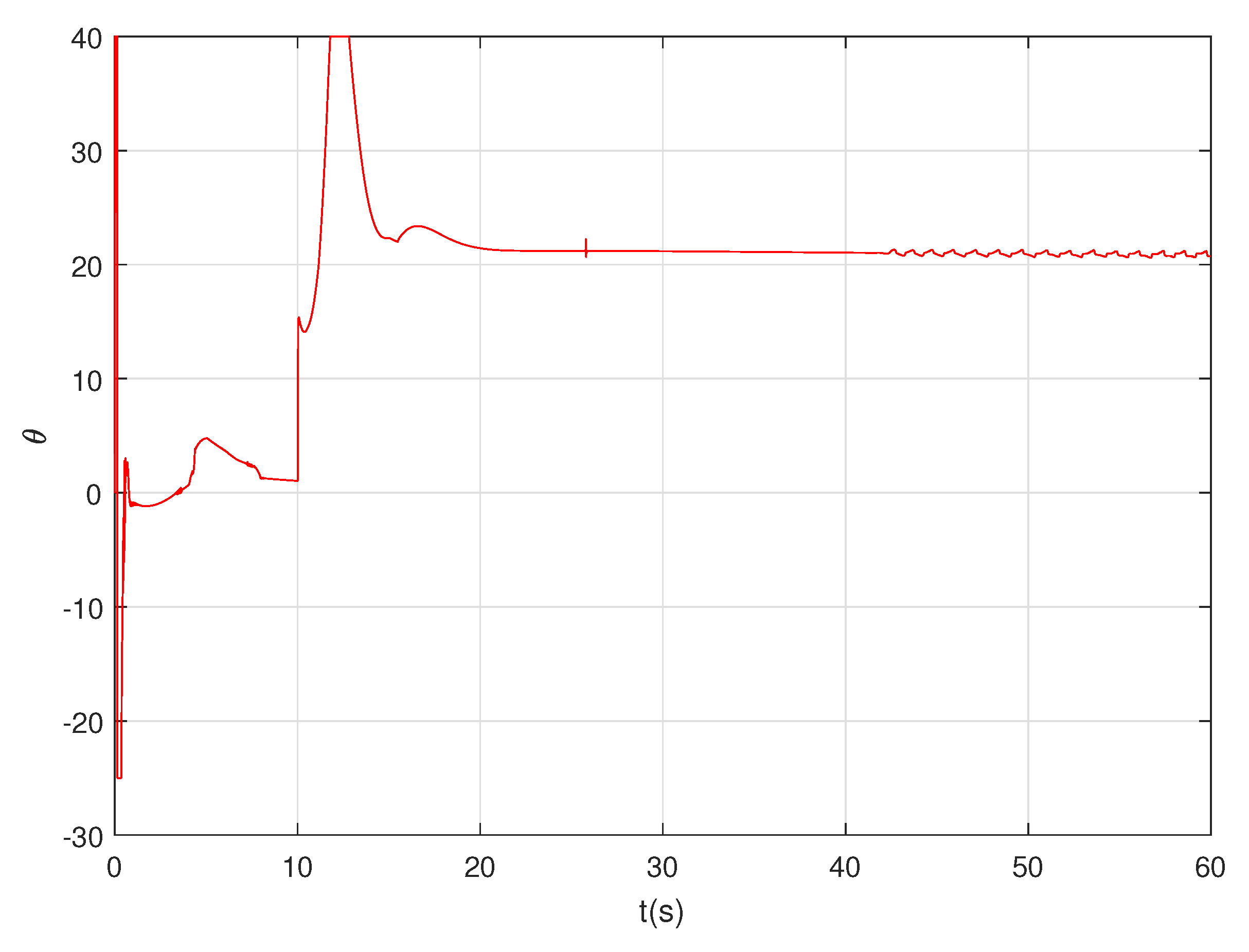
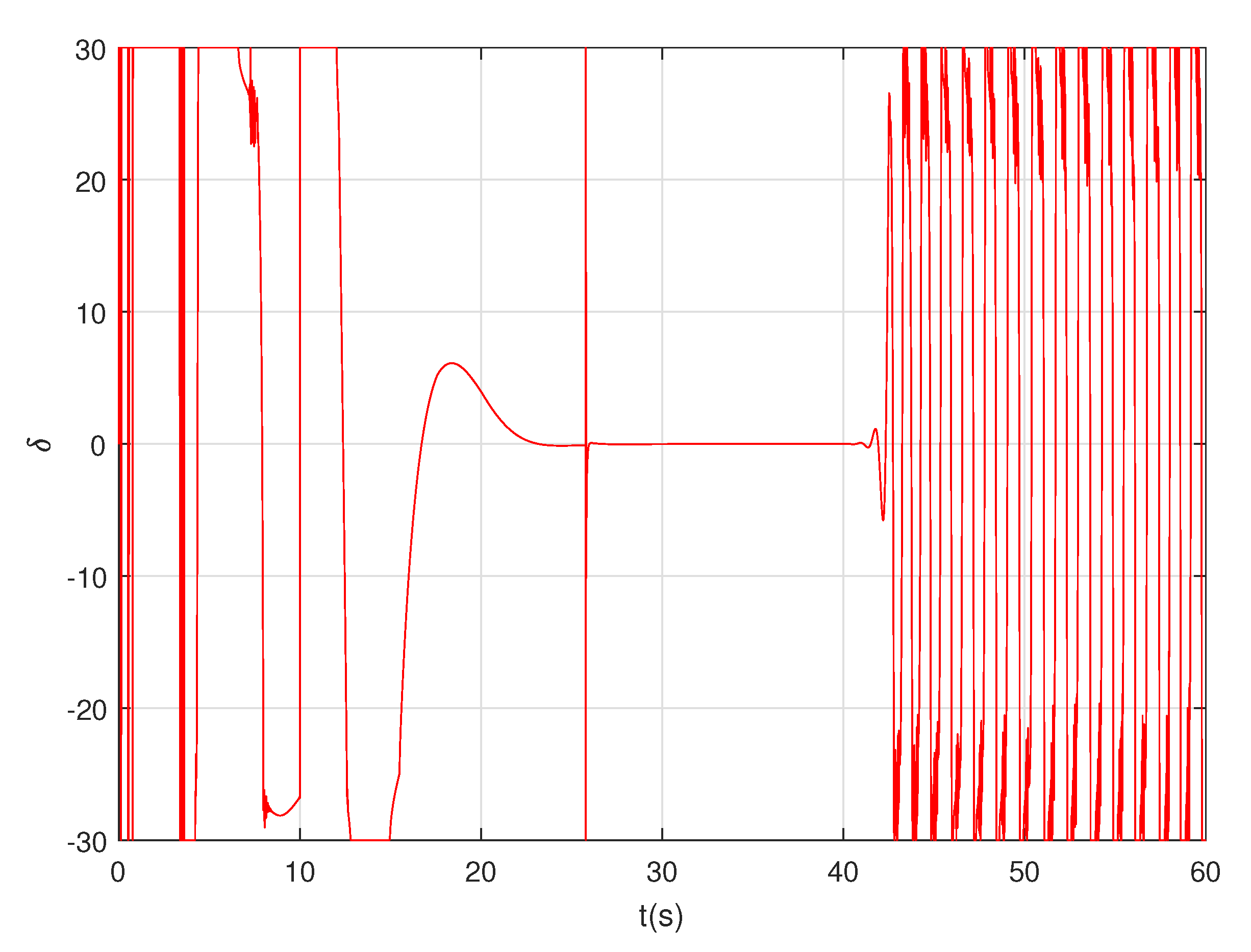
Proof. 

To facilitate the analysis, the positive definite Lyapunov function is chosen as:

$$\begin{array}{cc}\hfill V& =V_2+V_4\hfill \\ \hfill & =\frac{1}{2}{\left(z_e-{\delta }_{\Delta }\right)}^2+\frac{1}{2}{\xi }_u^2+\frac{1}{2}m{u}_e^2+\frac{1}{2}{{\tilde{W}}_u}^2+\frac{1}{2}{\psi }_e^2+\frac{1}{2}{\xi }_r^2+\frac{1}{2}{I}_{z}ln\frac{k_b^2}{k_b^2-r_e^2}+\frac{1}{2}{\tilde{W}}_r^2.\hfill \end{array}$$

(49)

Differentiating (49) with the help of (34) and (44), we have:

$$\begin{array}{cc}\dot{V}\le \hfill & -k_1{(z_e-{\sigma }_{\Delta })}^2-\frac{1}{2}{[{\xi }_u-c_u(z_e-{\sigma }_{\Delta })]}^2-\frac{1}{2}{[{\xi }_u-b_u\Delta {\alpha }_u]}^2\hfill \\ \hfill & -({\alpha }_u-1){\xi }_u^2-k_2{u}_e^2-g_u\left(t\right)N_u\left({\zeta }_u\left(t\right)\right)\overline{u}-u_e\overline{u}+u_e{\epsilon }_u\left(x\right)-{\eta }_u{\tilde{W}}_u{\widehat{W}}_u\hfill \\ \hfill & -k_3{\psi }_e^2-\frac{1}{2}{[{\xi }_r-c_r{\psi }_e]}^2-\frac{1}{2}{[{\xi }_r-b_r\Delta {\alpha }_r]}^2-({\alpha }_r-1){\xi }_r^2-k_4{r}_e^2+r_e{\epsilon }_r\left(x\right)\hfill \\ \hfill & -g_r\left(t\right)N_r\left({\zeta }_r\left(t\right)\right)\overline{r}-r_e\overline{r}-{\eta }_r{\tilde{W}}_r{\widehat{W}}_r\hfill \end{array}$$

(50)

Utilizing the Yang inequality, we obtain

$$\begin{array}{cc}\hfill u_e{\epsilon }_u\left(x\right)& \le \frac{1}{2}{u}_e^2+\frac{1}{2}{\epsilon }_u^2\left(x\right)\le \frac{1}{2}{u}_e^2+\frac{1}{2}{\overline{\epsilon }}^2\hfill \end{array}$$

(51)

$$\begin{array}{cc}\hfill r_e{\epsilon }_r\left(x\right)& \le \frac{1}{2}{r}_e^2+\frac{1}{2}{\epsilon }_r^2\left(x\right)\le \frac{1}{2}{r}_e^2+\frac{1}{2}{\overline{\epsilon }}^2\hfill \end{array}$$

(52)

$$\begin{array}{c}\hfill -{\eta }_{u,r}{\tilde{W}}_{u,r}{\widehat{W}}_{u,r}\le -\frac{{\eta }_{u,r}}{2}{\tilde{W}}_{u,r}^2+\frac{{\eta }_{u,r}}{2}{\widehat{W}}_{u,r}^2\end{array}$$

(53)

Subsequently, substituting (49) and (51)–(53) into (50), and according the Lemma 2, we have:

$$\begin{array}{c}\hfill \dot{V}\le -\Lambda V+\sum _{k=u,r}\frac{1}{{\rho }_k}[g_k\left(t\right)N_k\left({\zeta }_k\left(t\right)\right)+1]\dot{{\zeta }_k}\left(t\right)+\Gamma \end{array}$$

(54)

where

$$\begin{array}{c}\hfill \Lambda =min\{2k_1,2({\alpha }_u-1),\frac{2k_2-1}{m},{\eta }_{u,r},2k_3,2({\alpha }_r-1),\frac{2k_4}{I_z}\}\end{array}$$

$$\begin{array}{c}\hfill \Gamma =\frac{{\eta }_{u,r}}{2}{\widehat{W}}_{u,r}^2+{\overline{\epsilon }}^2.\end{array}$$

Taking the integration of (54) over the time $[0,t]$, we get:

$$\begin{array}{cc}\hfill V\le & \sum _{k=u,r}\frac{e^{-\Lambda t}}{{\rho }_k}{\int }_0^t[g_k\left(t\right)N_k+1]\dot{{\zeta }_k}\left(\lambda \right)e^{\Lambda \lambda }d\lambda -V\left(0\right)e^{-\Lambda t}+\frac{\Gamma }{\Lambda }.\hfill \end{array}$$

(55)

Applying Lemma 2 to (55), here $k=u,r$, then we draw the conclusion that $N_k\left({\zeta }_k\left(t\right)\right)$, $V\left(t\right)$, $e^{-\Lambda t}{\int }_0^t\dot{{\zeta }_k}\left(\lambda \right)e^{\Lambda \lambda }d\lambda$, $e^{-\Lambda t}{\int }_0^t{g}_k\left(t\right)N_k\left({\zeta }_k\left(\lambda \right)\right)\dot{{\zeta }_k}\left(\lambda \right)e^{\Lambda \lambda }d\lambda$ are bounded over $[0,t]$. ☐

Remark 4.

To improve the efficiency of selecting the parameters for design, the parameters$k_1,k_2,k_3,k_4$in the controller are required to be positive definite. The designed parameter${\eta }_{u,r}$in (38) and (48) are positive constants; and${\rho }_{u,r}$in (37) and (47) is defined as positive definite. For the given parameters$k_1,k_2,k_3,k_4,{\eta }_{u,r},{\rho }_{u,r}$, if the designed gain${\eta }_{u,r}$is set smaller but$k_1,k_2,k_3,k_4,and{\rho }_{u,r}$are chosen as larger, then the tracking error can be small.

4. Simulations

In this section, the analysis of the simulation results for an ACV is described. The ACV parameters are provided from [11], which are listed in

Table 1. Main particulars of ACV.

Variable	Value	Variable	Value
$m\left(kg\right)$	40,000	$I_z\left(kg{m}^2\right)$	$1.8\times {10}^6$
$I_x\left(kg{m}^2\right)$	$2.5\times {10}^5$	$S_{PP}\left(m^2\right)$	45
$S_{LP}\left(m^2\right)$	93	$S_{HP}\left(m^2\right)$	260
$Q(m^3/s)$	140.8	$S_c\left(m^2\right)$	212
$l_{sk}\left(m\right)$	65	$B_c\left(m\right)$	8.9
$h_m\left(m\right)$	2.4	$l_c\left(m\right)$	23.6
$h\left(m\right)$	1	$H_{hov}\left(m\right)$	5.9
$V_w\left(knot\right)$	5	${\beta }_w\left(deg\right)$	45

.

To verify the effectiveness of the proposed controller, we approximate the nonlinear relationships between the actuator’s input and output to constant values and adopt the backstepping controller for comparison. The backstepping controller is designed as:

$${\theta }_{backstepping}=0.5\overline{u}$$

$$\overline{u}=-k_2{u}_e-mvr+d_{11}u+d_{11}v-{\widehat{W}}_u{H}_u\left(x\right)+(z_e-{\delta }_{\Delta })cos\left({\psi }_e\right)+m{\dot{\alpha }}_u$$

$${\dot{\widehat{W}}}_u=-{\eta }_u{\widehat{W}}_u-u_e{H}_u\left(x\right)$$

$$\begin{array}{c}\hfill {\delta }_{backstepping}=0.07\left(t\right))\overline{r}\end{array}$$

$$\begin{array}{cc}\hfill \overline{r}=& -k_4{r}_e+m{\dot{\alpha }}_r-\left(k_b^2-r_e^2\right){\psi }_e+d_{41}u+d_{42}v+d_{44}r-N_{res}-{\widehat{W}}_r{H}_r\left(x\right)\hfill \end{array}$$

$$\begin{array}{c}\hfill {\dot{\widehat{W}}}_r=-{\eta }_r{\widehat{W}}_r-(r_e/(k_b^2-r_e^2))H_r\left(x\right)\end{array}$$

The desired trajectory is composed with a straight line and a circular arc.The trajectory is generated by choosing $u_d=30knots$, $v_d=0$, $p_d=0$, $r_d=0rad/s$ for $0s\le t\le 10s$ and $r_d=0.1rad/s$ for $10s\le t\le 60s$. The ACV initial state variables are set as $\eta \left(0\right)={[0,0,0,30deg]}^T$, ${\nu }_{(}{0)=[30knots,0,0,0]}^T$, ${\eta }_d\left(0\right)={[0,0,0,30deg]}^T$. The Nussbaum function $N\left(s\right)=s^{2}cos\left(s\right)$ is introduced. The controller and update parameters are set as ${\sigma }_{\Delta }=0.02$, $k_1=0.35$, $k_2=0.1$, $k_3=1.5*Mass$, $k_4=11$.

The simulation results are shown in Figure 5, Figure 6, Figure 7, Figure 8, Figure 9, Figure 10, Figure 11, Figure 12 and Figure 13. In this section, we refer to the controller designed in this article as the Nussbaum controller and the contrast controller as the backstepping controller. Figure 5 shows the trajectory tracking curves of the two controllers in the Earth coordinate system. The Nussbaum controller has a better tracking effect than the backstepping controller. The total position error $z_e$ and yaw error ${\psi }_e$ are presented in Figure 6. The position error curve illustrates that the Nussbaum controller converges faster and has a smaller amplitude. The partial enlarged view of the yaw error curve shows that the backstepping controller has periodic oscillations. The ACV position errors in the surge and sway directions are shown in Figure 7, which demonstrate that the proposed controller has a faster transient response and higher tracking precision compared to the backstepping controller. The virtual velocity tracking results are plotted in Figure 8. We can see that the surge velocity error under the Nussbaum controller can converge to near zero and remain stable with fast speed. Since both controllers introduce BLF to constrain the slew rate error, the virtual yaw rate errors are limited to a safe range, which can avoid side slip and tail swing phenomena caused by changes in the yaw rate that are too fast. Figure 9 and Figure 10 show the evolution of the Nussbaum parameters about the pitch angle and rudder angle, respectively. Figure 11 is the roll angle curve. Due to the higher accuracy of the controller proposed in this paper, the control force is greater at the switch between the straight line and the curve. Therefore, there is a greater roll angle fluctuation at approximately 10 s. However, the roll angles are generally within three degrees in engineering practice. It can be seen that both controllers can guarantee safe navigation. Figure 12 and Figure 13 are the input curves of pitch angle and rudder angle.

5. Conclusions

In this paper, an adaptive trajectory tracking safety controller based on the Nussbaum function and BLF has been designed for an ACV combing a RBFNN system and an auxiliary system in the presence of unknown effective input parameters, yaw rate error constraint and wind disturbance. The proposed control scheme depends on the four DOF vector model of the ACV. It can not only highlight the different characteristics between the ACV and ordinary surface ships but also promote the research method of surface ships for the ACV. The adaptive Nussbaum gain-based approach is incorporated with the backstepping scheme to handle the unknown effective input parameters. Furthermore, the yaw rate error has been constrained to a prescribed region by introducing a BLF into the backstepping procedure. The command filter and auxiliary systems are adopted to avoid the complicated calculation of the derivative of the virtual control laws. By combining with RBFNN, the controller can deal with the uncertainty of the ACV’s complex model and wind disturbance. The simulation results and comparisons demonstrate the effectiveness of the proposed control scheme.

References

1. Yifan, Y.; Jun, L.; Zhou, X.L. A review of research on the control of fully-lift hovercraft. Ship Sci. Technol. 2012, 34, 11–15. [Google Scholar]
2. Pagotti, A.P.; Rafikova, E.; Rafikov, M. SDRE Trajectory Tracking Control for a Hovercraft Autonomous Vehicle: Selected Papers of the XVII International Symposium on Dynamic Problems of Mechanics. In Proceedings of DINAME 2017; Springer: Cham, Switzerland, 2019. [Google Scholar]
3. Yun, L.; Bliault, A. Theory Design of Air Cushion Craft; Butterworth-Heinemann: Oxford, UK, 2000. [Google Scholar]
4. Shojaei, K. Neural adaptive robust control of underactuated marine surface vehicles with input saturation. Appl. Ocean Res. 2015, 53, 267–278. [Google Scholar] [CrossRef]
5. Aranda, J.; Chaos, D.; Dormido-Canto, S.; Muñoz, R.; Diaz, J.M. Benchmark control problems for a non-linear underactuated hovercraft:a simulation laboratory for control testing. IFAC Proc. Vol. 2006, 39, 463–468. [Google Scholar] [CrossRef]
6. Rigatos, G.G.; Raffo, G.V. Input-output linearizing control of the underactuated hovercraft using the derivative-free nonlinear Kalman filter. Unmanned Syst. 2015, 39, 127–142. [Google Scholar] [CrossRef]
7. Morales, R.; Sira-Ramírez, H.; Somolinos, J.A. Linear active disturbance rejection control of the hovercraft vessel model. Ocean Eng. 2015, 39, 100–108. [Google Scholar] [CrossRef] [Green Version]
8. Zhao, J.; Pang, J. Trajectory control of underactuated hovercraft. In Proceedings of the IEEE 2010 8th World Congress on Intelligent Control and Automation, Jinan, China, 7–9 July 2010; pp. 3904–3907. [Google Scholar]
9. Aranda, J.A.; García, D.C.; Canto, S.D.; Mansilla, R.M.; Martínez, J.M.D. A control for tracking and stabilization o faunderactuated non-linear RC hovercraft. In Proceedings of the 7th IFAC Conference Manoeuvring Control Marine Crafts (MCM), Lisbon, Portugal, 20–22 September 2006. [Google Scholar]
10. Sira-Ramirez, H. Dynamic second-order sliding mode control of the hovercraft vessel. IEEE Trans. Control Syst. Technol. 2002, 10, 860–865. [Google Scholar] [CrossRef]
11. Hua, F. Analysis and Consideration on Safety of All-Lift Hovercraft; SHIP & BOAT: Shanghai, China, 2008. [Google Scholar]
12. Fu, M.Y.; Gao, S. Human-Centered Automatic Tracking System for Underactuated Hovercraft Based on Adaptive Chattering-Free Full-Order Terminal Sliding Mode Control. IEEE Access 2018, 6, 37883–37892. [Google Scholar] [CrossRef]
13. Fu, M.Y.; Gao, S. Design of driver assistance system for air cushion vehicle with uncertainty based on model knowledge neural network. Ocean. Eng. 2019, 172, 296–307. [Google Scholar] [CrossRef]
14. Bechlioulis, C.P.; Karras, G.C.; Heshmati-Alamdari, S.; Kyriakopoulos, K.J. Trajectory Tracking With Prescribed Performance for Underactuated Underwater Vehicles Under Model Uncertainties and External Disturbances. IEEE Trans. Control. Syst. Technol. 2017, 25, 429–440. [Google Scholar] [CrossRef]
15. Garcia, G.; Keshmiri, S. Nonlinear Model Predictive Controller for Navigation, Guidance and Control of a Fixed-Wing UAV. In Proceedings of the Aiaa Guidance, Navigation, &Control Conference, Portland, OR, USA, 8–11 August 2013. [Google Scholar]
16. He, W.; Yin, Z.; Sun, C. Adaptive Neural Network Control of a Marine Vessel With Constraints Using the Asymmetric Barrier Lyapunov Function. IEEE Trans. Cybern. 2017, 47, 1641–1651. [Google Scholar] [CrossRef]
17. Kogiso, K.; Hirata, K. Reference Governor for Constrained Systems with Time-Varying References; North-Holland Publishing Co.: Amsterdam, The Netherlands, 2009. [Google Scholar]
18. Herrmann, G.; Turner, M.C.; Postlethwaite, I. A robust override scheme enforcing strict output constraints for a class of strictly proper systems. IFAC Proc. Vol. 2005, 38, 49–54. [Google Scholar] [CrossRef]
19. Hatanaka, T.; Takaba, K. Computations of probabilistic output admissible set for uncertain constrained systems. Automatica 2008, 44, 479–487. [Google Scholar] [CrossRef]
20. Liu, Z.; Geng, C.; Zhang, J. Model predictive controller design with disturbance observer for path following of unmanned surface vessel. In Proceedings of the IEEE International Conference on Mechatronics & Automation, Takamatsu, Japan, 6–9 August 2017. [Google Scholar]
21. Kostarigka, A.K.; Rovithakis, G.A. Prescribed Performance Output Feedback/Observer-Free Robust Adaptive Control of Uncertain Systems Using Neural Networks. IEEE Trans. Syst. Man Cybern. Part Cybern. Publ. IEEE Syst. Man Cybern. Soc. 2011, 41, 1483–1494. [Google Scholar] [CrossRef] [PubMed]
22. Kostarigka, A.K.; Rovithakis, G.A. Adaptive dynamic output feedback neural network control of uncertain MIMO nonlinear systems with prescribed performance. IEEE Trans. Neural Netw. Learn. Syst. 2012, 23, 138–149. [Google Scholar] [CrossRef]
23. Yin, Z.; He, W.; Yang, C. Tracking control of a marine surface vessel with full-state constraints. Int. J. Syst. Sci. 2017, 48, 535–546. [Google Scholar] [CrossRef]
24. Zheng, Z.; Huang, Y.; Xie, L.; Zhu, B. Adaptive Trajectory Tracking Control of a Fully Actuated Surface Vessel With Asymmetrically Constrained Input and Output. IEEE Trans. Control Syst. Technol. 2017, 26, 1851–1859. [Google Scholar] [CrossRef]
25. Zheng, Z.; Feroskhan, M. Path Following of a Surface Vessel With Prescribed Performance in the Presence of Input Saturation and External Disturbances. IEEE/ASME Trans. Mechatron. 2017, 22, 2564–2575. [Google Scholar] [CrossRef]
26. Zhang, G.Q.; Huang, C.F.; Wu, X.X.; Zhang, X.K. Adaptive finite-time control of ship dynamic positioning considering uncertain gain of servo system. Acta Autom. Sin. 2018, 44, 1907–1912. [Google Scholar]
27. Morse, A.S. Recent problems in parameter adaptive control. Model. Autom. 1982, 3, 733–740. [Google Scholar]
28. Chen, C.; Liu, Z.; Xie, K.; Liu, Y.; Zhang, Y.; Chen, C.P. Adaptive Fuzzy Asymptotic Control of MIMO Systems with Unknown Input Coefficients Via a Robust Nussbaum Gain based Approach. IEEE Trans. Fuzzy Syst. 2016, 25, 1252–1263. [Google Scholar] [CrossRef]
29. Zhang, J.; Mu, X.W. Nussbaum function and its application in system stabilization. Math. Pract. Theory 2017, 20, 239–245. [Google Scholar]
30. Chen, C.; Liu, Z.; Zhang, Y.; Chen, C.P.; Xie, S.L. Adaptive control of MIMO mechanical systems with unknown actuator nonlinearities based on the Nussbaum gain approach. IEEE/CAA J. Autom. Sin. 2016. [Google Scholar] [CrossRef]
31. Wang, D.; Fu, M.; Ge, S.S.; Li, D. Velocity Free Platoon Formation Control for Unmanned Surface Vehicles with Output Constraints and Model Uncertainties. Appl. Sci. 2020, 10, 1118. [Google Scholar] [CrossRef] [Green Version]
32. Fossen, T.I.; Strand, J.P. Passive nonlinear observer design for ships using Lyapunov methods: Full-scale experiments with a supply vessel. Automatica 1999, 35, 3–16. [Google Scholar] [CrossRef]
33. Krstic, M.; Kokotovic, P.V.; Kanellakopoulos, I. Nonlinear and Adaptive Control Design; Wiley: Hoboken, NJ, USA, 1995. [Google Scholar]
34. Sepulchre, R.; Jankovic, M.; Kokotovic, P.V. Constructive Nonlinear Control; Springer: New York, NY, USA, 2012. [Google Scholar]
Figure 1. Scheme diagram of the trajectory tracking system of Air Cushion Vehicle (ACV).
Applsci 10 05695 g001
Figure 2. Scheme diagram of the trajectory tracking system of ACV.
Applsci 10 05695 g002
Figure 3. Tracking errors.
Applsci 10 05695 g003
Figure 4. The filter block diagram.
Applsci 10 05695 g004
Figure 5. The trajectory of ACV in earth coordinate.
Applsci 10 05695 g005
Figure 6. Tracking error.
Applsci 10 05695 g006
Figure 7. Position error of trajectory tracking.
Applsci 10 05695 g007
Figure 8. Surge speed error and yaw rate error of trajectory tracking.
Applsci 10 05695 g008
Figure 9. Nussbaum parameters.
Applsci 10 05695 g009
Figure 10. Nussbaum parameters.
Applsci 10 05695 g010
Figure 11. Roll angle of trajectory tracking.
Applsci 10 05695 g011
Figure 12. Pitch angle of the air propeller.
Applsci 10 05695 g012
Figure 13. Angle of the air rudder.
Applsci 10 05695 g013