A New Adaptive Spatial Filtering Method in the Wavelet Domain for Medical Images


Abstract
1. Introduction
1.1. State of the Art
1.2. Scope and Objectives
2. Materials and Methods
2.1. Theoretical Background
- -
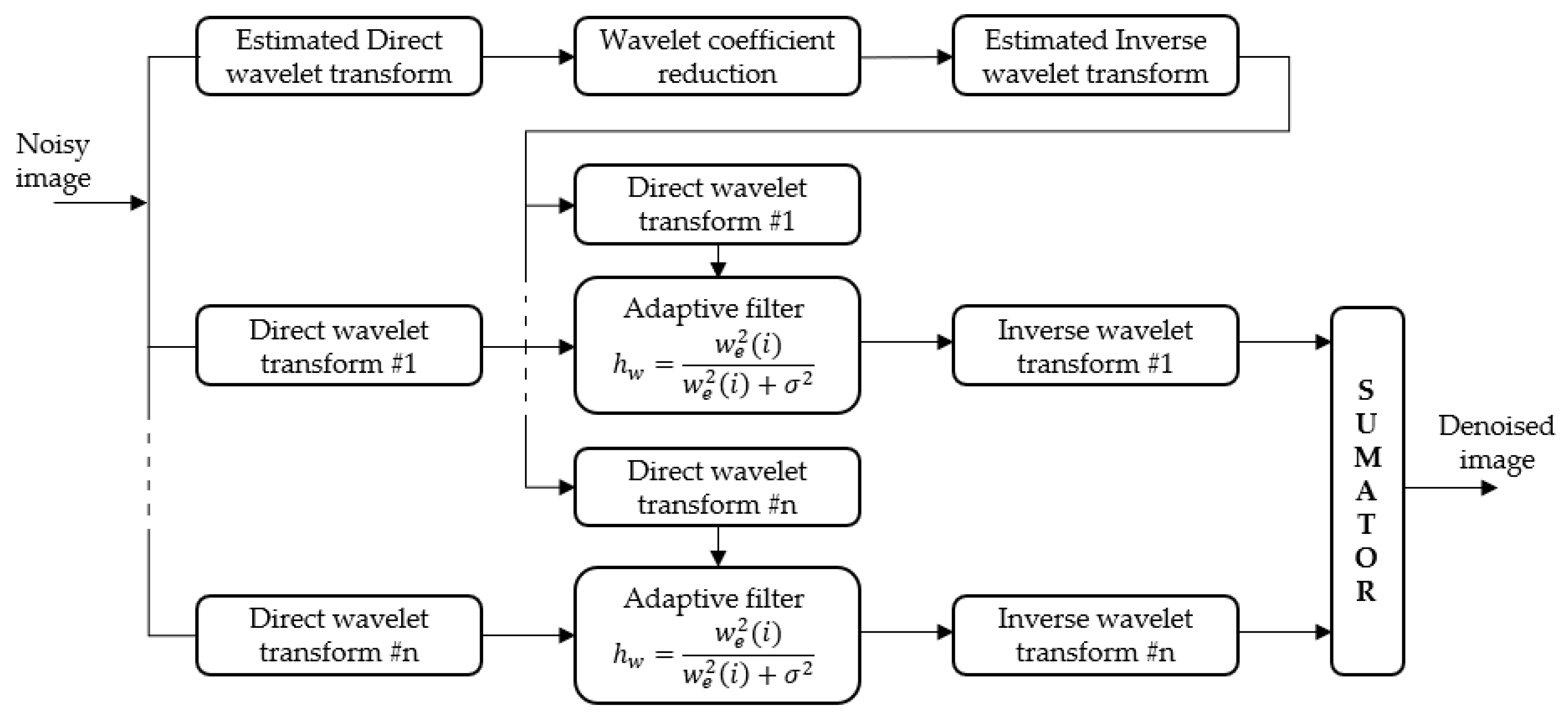
- As in many other noise reduction methods using dyadic wavelet transformation, the lowest resolution sub-band is not processed (represented in blue in Figure 1);
- -
- Each of the three low-resolution detail sub-bands (corresponding to wavelet decomposition level 3, red in Figure 1) is processed by soft truncation; the threshold value for each sub-band is determined by modeling the distribution of its coefficients by a Laplace distribution of zero mean and dispersion:where:is the Gaussian noise dispersion, M being the number of coefficients in the considered sub-band and w the wavelet coefficients of the noise-degraded image.
- -
- in the case of the other detail sub-bands (corresponding to wavelet decomposition levels 2 and 1 and represented by the colors green and white in Figure 1), the significance map is drawn up based on the absolute value of the parent coefficient corresponding to each coefficient belonging to these sub-bands (in Figure 1, the relation descending coefficient—parent coefficient is also represented); thus, if the value of the parent coefficient is higher than a threshold value T, the coefficient considered is classified as significant, otherwise it is classified as insignificant; the two classes of coefficients, having different informational significance, have different statistical properties, therefore they are processed differently:
- o
- the significant classified coefficients are soft truncated, the threshold value used is determined based on the modeling of their distribution with a Laplace distribution of zero mean and dispersion:where:sig representing the significance map, and the number of coefficients in this map.
- o
- insignificant classified coefficients have small values and represent smooth regions; for each such coefficient the dispersion is estimated using a window of dimensions 5 × 5, but from which the significant coefficients are eliminated; if represents the thus estimated dispersion of the signal, then the a posteriori maximum probability estimator will be:
2.2. Algorithm Proposed in This Work
- For each scale, from ;
- We determine the data set , with the following itterative process:
- B1.
- We compute and
- B2.
- We then compute the correlation and wavelet factors:
- B3.
- We perform the scaling:
- B4.
- We identify the contour location by verifying if the following condition is met:Additionally, for each location identified as a contour, we execute:
- B5.
- We then test the stopping condition of the iterative process:
3. Results and Discussions
- (A)
- By integrally applying the proposed algorithm in translation invariant form, mediating the results obtained by applying all three processing steps on the cyclic displacements of the input image;
- (B)
- By partially applying the proposed algorithm (only steps 1 and 2) in the translation invariant form and performing the correction according to the contour map only on the result thus obtained.
- Improving image quality by selectively eliminating disturbing information, such as noise, and eliminating other defects caused by the acquisition device by using adaptive filters.
- Highlighting areas of interest by adjusting light intensity and contrast and accentuating contours and textures.
- Improving the ability to detect edges by using the image fusion method based on the wavelet algorithm.
- Developing new methods for evaluating segmentation.
- Evaluating the performance of edge detection methods using operators that analyze the structural similarity of images.
- The use of high-performance algorithms of Artificial Intelligence to perform sub-pixelation calculations and the transition from macroscopic analysis currently used to microscopic analysis for the analysis of tumors generated by cancer by analyzing medical images.
4. Conclusions
Author Contributions
Funding
Acknowledgments
Conflicts of Interest
Appendix A

| a. Boat image, 256 × 256 pixels. | ||||||||||||
| Threshold Value | ||||||||||||
| Initial Image | PSNR = 26.07 dB | C = 64.61% | Initial Image | PSNR = 20.03 dB | C = 47.09% | |||||||
| Second Processing Stage | PSNR = 30.88 dB | C = 64.29% | Second Processing Stage | PSNR = 27.10 dB | C = 49.53% | |||||||
| Ideal Contour Map | Real Contour Map | Filtered Contour Map | Ideal Contour Map | Real Contour Map | Filtered Contour Map | |||||||
| PSNR (dB) | C (%) | PSNR (dB) | C (%) | PSNR (dB) | C (%) | PSNR (dB) | C (%) | PSNR (dB) | C (%) | PSNR (dB) | C (%) | |
| 0.050 | 30.93 | 65.17 | 30.29 | 64.38 | 30.39 | 65.03 | 26.94 | 51.75 | 25.04 | 51.75 | 24.85 | 51.15 |
| 0.075 | 30.94 | 64.87 | 30.68 | 64.90 | 30.79 | 64.98 | 27.12 | 50.16 | 25.47 | 50.21 | 25.43 | 50.00 |
| 0.100 | 30.93 | 64.90 | 30.82 | 65.12 | 30.84 | 64.75 | 27.16 | 51.37 | 25.96 | 50.19 | 26.24 | 49.90 |
| 0.150 | 30.90 | 64.66 | 30.86 | 64.27 | 30.86 | 64.30 | 27.16 | 49.56 | 26.74 | 49.76 | 27.00 | 50.23 |
| 0.175 | 30.89 | 64.59 | 30.87 | 64.58 | 30.87 | 64.32 | 27.14 | 49.24 | 26.93 | 50.26 | 27.06 | 50.42 |
| 0.200 | 30.88 | 64.51 | 30.87 | 64.45 | 30.87 | 64.41 | 27.14 | 49.03 | 27.02 | 49.66 | 27.07 | 50.03 |
| 0.225 | 30.88 | 64.38 | 30.87 | 64.32 | 30.87 | 64.38 | 27.13 | 49.11 | 27.06 | 50.10 | 27.08 | 49.81 |
| 0.250 | 30.88 | 64.43 | 30.87 | 64.40 | 30.87 | 64.30 | 27.12 | 48.95 | 27.07 | 49.29 | 27.08 | 49.00 |
| b. Calendar image, 256 × 256 pixels. | ||||||||||||
| Threshold Value | ||||||||||||
| Initial Image | PSNR = 26.00 dB | C = 70.01% | Initial Image | PSNR = 21.11 dB | C = 58.73% | |||||||
| Second Processing Stage | PSNR = 28.15 dB | C = 74.42% | Second Processing Stage | PSNR = 23.11 dB | C = 58.53% | |||||||
| Ideal Contour Map | Real Contour Map | Filtered Contour Map | Ideal Contour Map | Real Contour Map | Filtered Contour Map | |||||||
| PSNR (dB) | C (%) | PSNR (dB) | C (%) | PSNR (dB) | C (%) | PSNR (dB) | C (%) | PSNR (dB) | C (%) | PSNR (dB) | C (%) | |
| 0.050 | 28.24 | 71.23 | 28.03 | 70.59 | 28.03 | 70.82 | 23.56 | 58.70 | 23.13 | 58.37 | 23.09 | 58.15 |
| 0.075 | 28.25 | 75.22 | 28.14 | 71.06 | 28.15 | 71.19 | 23.55 | 58.51 | 23.23 | 57.60 | 23.24 | 58.07 |
| 0.100 | 28.24 | 75.40 | 28.17 | 75.40 | 28.18 | 75.20 | 23.50 | 58.32 | 23.31 | 57.54 | 23.33 | 57.34 |
| 0.150 | 28.21 | 74.99 | 28.18 | 75.55 | 28.18 | 75.49 | 23.40 | 57.61 | 23.33 | 57.38 | 23.31 | 57.35 |
| 0.175 | 28.20 | 74.72 | 28.17 | 75.23 | 28.17 | 75.15 | 23.35 | 57.44 | 23.30 | 57.52 | 23.27 | 57.34 |
| 0.200 | 28.19 | 74.72 | 28.17 | 74.66 | 28.17 | 74.59 | 23.31 | 57.25 | 23.27 | 57.35 | 23.22 | 57.30 |
| 0.225 | 28.18 | 74.72 | 28.17 | 74.75 | 28.16 | 74.73 | 23.27 | 56.55 | 23.22 | 57.05 | 23.19 | 57.08 |
| 0.250 | 28.17 | 74.75 | 28.16 | 74.77 | 28.16 | 74.65 | 23.23 | 56.58 | 23.19 | 56.67 | 23.16 | 56.92 |
| c. Wheel image, 256 × 256 pixels. | ||||||||||||
| Threshold Value | ||||||||||||
| Initial Image | PSNR = 26.22 dB | C = 73.81% | Initial image | PSNR = 20.40 dB | C = 58.49% | |||||||
| Second Processing Stage | PSNR = 28.44 dB | C = 72.63% | Second Processing Stage | PSNR = 24.61 dB | C = 57.18% | |||||||
| Ideal Contour Map | Real Contour Map | Filtered Contour Map | Ideal Contour Map | Real Contour Map | Filtered Contour Map | |||||||
| PSNR (dB) | C (%) | PSNR (dB) | C (%) | PSNR (dB) | C (%) | PSNR (dB) | C (%) | PSNR (dB) | C (%) | PSNR (dB) | C (%) | |
| 0.050 | 28.51 | 73.90 | 28.29 | 73.80 | 28.29 | 73.44 | 24.53 | 60.49 | 23.91 | 59.35 | 23.83 | 59.48 |
| 0.075 | 28.53 | 73.98 | 28.37 | 73.54 | 28.39 | 73.53 | 24.70 | 60.37 | 24.08 | 59.07 | 24.04 | 59.47 |
| 0.100 | 28.51 | 73.49 | 28.42 | 73.54 | 28.43 | 73.13 | 24.74 | 59.82 | 24.25 | 59.45 | 24.33 | 59.87 |
| 0.150 | 28.48 | 72.83 | 28.44 | 72.97 | 28.44 | 72.73 | 24.74 | 58.93 | 24.51 | 59.25 | 24.58 | 59.18 |
| 0.175 | 28.47 | 72.83 | 28.44 | 72.71 | 28.44 | 72.54 | 24.71 | 58.88 | 24.56 | 58.93 | 24.60 | 58.39 |
| 0.200 | 28.46 | 72.54 | 28.44 | 72.62 | 28.44 | 72.54 | 24.69 | 58.76 | 24.60 | 58.07 | 24.60 | 57.50 |
| 0.225 | 28.45 | 72.83 | 28.44 | 72.54 | 28.44 | 72.57 | 24.67 | 58.47 | 24.61 | 58.19 | 24.60 | 57.36 |
| 0.250 | 28.45 | 72.68 | 28.44 | 72.62 | 28.44 | 72.57 | 24.66 | 58.20 | 24.61 | 57.97 | 24.60 | 57.48 |
| d. Aerial image, 256 × 256 pixels. | ||||||||||||
| Threshold Value | ||||||||||||
| Initial Image | PSNR = 26.04 dB | C = 70.12% | Initial Image | PSNR = 20.15 dB | C = 54.02% | |||||||
| Second Processing Stage | PSNR = 28.16 dB | C = 67.43% | Second Processing Stage | PSNR = 24.23 dB | C = 49.76% | |||||||
| Ideal Contour Map | Real Contour Map | Filtered Contour Map | Ideal Contour Map | Real Contour Map | Filtered Contour Map | |||||||
| PSNR (dB) | C (%) | PSNR (dB) | C (%) | PSNR (dB) | C (%) | PSNR (dB) | C (%) | PSNR (dB) | C (%) | PSNR (dB) | C (%) | |
| 0.050 | 28.19 | 69.32 | 27.96 | 68.23 | 27.94 | 68.29 | 24.12 | 53.90 | 23.50 | 52.99 | 23.43 | 53.65 |
| 0.075 | 28.32 | 68.24 | 28.05 | 68.23 | 28.06 | 68.76 | 24.29 | 53.75 | 23.64 | 52.88 | 23.61 | 53.66 |
| 0.100 | 28.22 | 67.69 | 28.11 | 67.86 | 28.13 | 67.90 | 24.34 | 53.45 | 23.80 | 52.86 | 23.85 | 53.01 |
| 0.150 | 28.20 | 67.40 | 28.15 | 67.12 | 28.15 | 67.97 | 24.34 | 52.27 | 24.07 | 52.10 | 24.16 | 51.93 |
| 0.175 | 28.19 | 67.07 | 28.15 | 66.92 | 28.15 | 66.75 | 24.32 | 51.55 | 24.14 | 51.78 | 24.20 | 51.21 |
| 0.200 | 28.18 | 68.11 | 28.15 | 66.73 | 28.16 | 67.77 | 24.30 | 50.97 | 24.19 | 51.49 | 24.22 | 51.04 |
| 0.225 | 28.17 | 68.10 | 28.15 | 68.04 | 28.16 | 67.67 | 24.28 | 50.65 | 24.21 | 50.98 | 24.22 | 50.59 |
| 0.250 | 28.17 | 68.00 | 28.15 | 68.02 | 28.16 | 67.52 | 24.26 | 50.51 | 24.21 | 50.49 | 24.22 | 50.11 |
| e. Camera image, 256 × 256 pixels. | ||||||||||||
| Threshold Value | ||||||||||||
| Initial Image | PSNR = 26.20 dB | C = 65.80% | Initial Image | PSNR = 20.43 dB | C = 51.32% | |||||||
| Second Processing Stage | PSNR = 30.77 dB | C = 64.97% | Second Processing Stage | PSNR = 26.74 dB | C = 48.90% | |||||||
| Ideal Contour Map | Real Contour Map | Filtered Contour Map | Ideal Contour Map | Real Contour Map | Filtered Contour Map | |||||||
| PSNR (dB) | C (%) | PSNR (dB) | C (%) | PSNR (dB) | C (%) | PSNR (dB) | C (%) | PSNR (dB) | C (%) | PSNR (dB) | C (%) | |
| 0.050 | 30.79 | 66.39 | 30.24 | 66.51 | 30.33 | 67.02 | 26.75 | 53.29 | 25.23 | 52.60 | 25.06 | 52.79 |
| 0.075 | 30.80 | 66.63 | 30.58 | 66.06 | 30.66 | 66.77 | 26.87 | 51.63 | 25.59 | 52.30 | 25.95 | 52.14 |
| 0.100 | 30.80 | 66.37 | 30.70 | 65.58 | 30.72 | 66.04 | 26.88 | 51.42 | 26.04 | 51.38 | 26.26 | 52.01 |
| 0.150 | 30.78 | 65.78 | 30.73 | 65.58 | 30.74 | 65.43 | 26.83 | 50.33 | 26.56 | 50.69 | 26.69 | 50.28 |
| 0.175 | 30.78 | 65.70 | 30.74 | 65.62 | 30.75 | 65.45 | 26.81 | 50.02 | 26.66 | 50.43 | 26.69 | 49.92 |
| 0.200 | 30.77 | 65.60 | 30.75 | 65.49 | 30.75 | 65.47 | 26.79 | 49.94 | 26.72 | 49.63 | 26.71 | 49.53 |
| 0.225 | 30.77 | 65.29 | 30.75 | 65.41 | 30.75 | 65.35 | 26.78 | 49.80 | 26.72 | 49.80 | 26.71 | 49.29 |
| 0.250 | 30.76 | 65.33 | 30.75 | 65.35 | 30.75 | 65.37 | 26.76 | 49.92 | 26.71 | 49.80 | 26.70 | 49.47 |
| f. Goldhill image, 256 × 256 pixels. | ||||||||||||
| Threshold Value | ||||||||||||
| Initial Image | PSNR = 26.03 dB | C = 57.42% | Initial Image | PSNR = 20.11 dB | C = 42.43% | |||||||
| Second Processing Stage | PSNR = 29.37 dB | C = 58.92% | Second Processing Stage | PSNR = 25.89 dB | C = 40.30% | |||||||
| Ideal Contour Map | Real Contour Map | Filtered Contour Map | Ideal Contour Map | Real Contour Map | Filtered Contour Map | |||||||
| PSNR (dB) | C (%) | PSNR (dB) | C (%) | PSNR (dB) | C (%) | PSNR (dB) | C (%) | PSNR (dB) | C (%) | PSNR (dB) | C (%) | |
| 0.050 | 29.40 | 60.74 | 29.02 | 60.44 | 29.05 | 60.48 | 25.72 | 44.06 | 24.50 | 42.61 | 24.37 | 42.81 |
| 0.075 | 29.42 | 59.73 | 29.22 | 59.39 | 29.27 | 59.28 | 25.92 | 43.59 | 24.80 | 41.41 | 24.78 | 41.94 |
| 0.100 | 29.41 | 58.66 | 29.30 | 58.70 | 29.34 | 58.31 | 25.95 | 42.36 | 25.13 | 42.16 | 25.31 | 43.27 |
| 0.150 | 29.39 | 58.58 | 29.35 | 58.44 | 29.36 | 58.59 | 25.94 | 41.24 | 25.76 | 41.64 | 25.83 | 41.31 |
| 0.175 | 29.38 | 58.43 | 29.36 | 58.40 | 29.37 | 58.44 | 25.92 | 40.63 | 25.76 | 41.64 | 25.88 | 40.85 |
| 0.200 | 29.37 | 58.50 | 29.36 | 58.48 | 29.36 | 58.50 | 25.91 | 40.42 | 25.82 | 41.42 | 25.88 | 40.57 |
| 0.225 | 29.37 | 58.46 | 29.36 | 58.51 | 29.36 | 58.53 | 25.90 | 40.43 | 25.85 | 40.69 | 25.89 | 40.39 |
| 0.250 | 29.37 | 58.42 | 29.36 | 58.46 | 29.36 | 58.50 | 25.89 | 40.52 | 25.86 | 40.45 | 25.89 | 40.43 |
| g. Peppers image, 256 × 256 pixels. | ||||||||||||
| Threshold Value | ||||||||||||
| Initial Image | PSNR = 26.08 dB | C = 63.72% | Initial Image | PSNR = 20.16 dB | C = 49.46% | |||||||
| Second Processing Stage | PSNR = 30.52 dB | C = 64.25% | Second Processing Stage | PSNR = 26.74 dB | C = 47.43% | |||||||
| Ideal Contour Map | Real Contour Map | Filtered Contour Map | Ideal Contour Map | Real Contour Map | Filtered Contour Map | |||||||
| PSNR (dB) | C (%) | PSNR (dB) | C (%) | PSNR (dB) | C (%) | PSNR (dB) | C (%) | PSNR (dB) | C (%) | PSNR (dB) | C (%) | |
| 0.050 | 30.54 | 64.62 | 29.93 | 65.24 | 30.01 | 65.57 | 26.75 | 51.33 | 24.94 | 50.40 | 24.70 | 50.34 |
| 0.075 | 30.55 | 64.11 | 30.29 | 64.57 | 30.39 | 64.11 | 26.87 | 50.23 | 25.33 | 50.11 | 25.30 | 50.34 |
| 0.100 | 30.56 | 63.99 | 30.44 | 64.17 | 30.47 | 63.80 | 26.91 | 49.32 | 25.82 | 50.90 | 26.08 | 50.90 |
| 0.150 | 30.54 | 63.80 | 30.50 | 63.54 | 30.50 | 63.52 | 26.84 | 48.67 | 26.50 | 49.79 | 26.70 | 48.12 |
| 0.175 | 30.53 | 63.74 | 30.50 | 63.64 | 30.51 | 63.62 | 26.82 | 48.24 | 26.67 | 48.97 | 26.75 | 47.84 |
| 0.200 | 30.53 | 63.97 | 30.51 | 63.80 | 30.51 | 63.84 | 26.79 | 47.90 | 26.71 | 48.08 | 26.74 | 47.78 |
| 0.225 | 30.52 | 63.94 | 30.51 | 63.76 | 30.51 | 63.78 | 26.79 | 47.90 | 26.74 | 47.63 | 26.73 | 47.51 |
| 0.250 | 30.52 | 63.82 | 30.51 | 63.70 | 30.51 | 63.74 | 26.77 | 47.96 | 26.73 | 47.63 | 26.73 | 47.33 |
| h. Bridge image, 256 × 256 pixels. | ||||||||||||
| Threshold Value | ||||||||||||
| Initial Image | PSNR = 26.07 dB | C = 63.70% | Initial Image | PSNR = 20.14 dB | C = 47.13% | |||||||
| Second Processing Stage | PSNR = 27.65 dB | C = 62.68% | Second Processing Stage | PSNR = 23.46 dB | C = 44.56% | |||||||
| Ideal Contour Map | Real Contour Map | Filtered Contour Map | Ideal Contour Map | Real Contour Map | Filtered Contour Map | |||||||
| PSNR (dB) | C (%) | PSNR (dB) | C (%) | PSNR (dB) | C (%) | PSNR (dB) | C (%) | PSNR (dB) | C (%) | PSNR (dB) | C (%) | |
| 0.050 | 27.68 | 64.29 | 27.50 | 63.58 | 27.50 | 63.85 | 23.41 | 47.22 | 22.98 | 46.64 | 22.93 | 47.30 |
| 0.075 | 27.69 | 63.92 | 27.56 | 63.52 | 27.58 | 63.58 | 23.52 | 47.01 | 23.07 | 46.30 | 23.04 | 46.91 |
| 0.100 | 27.69 | 63.47 | 27.61 | 63.58 | 27.62 | 63.14 | 23.55 | 46.20 | 23.18 | 45.99 | 23.21 | 46.22 |
| 0.150 | 27.67 | 63.26 | 27.64 | 63.16 | 27.64 | 62.82 | 23.52 | 44.57 | 23.35 | 44.82 | 23.42 | 44.68 |
| 0.175 | 27.66 | 62.90 | 27.64 | 62.88 | 27.65 | 62.79 | 23.50 | 44.42 | 23.39 | 44.85 | 23.45 | 44.27 |
| 0.200 | 27.66 | 62.83 | 27.64 | 62.96 | 27.65 | 62.77 | 23.49 | 44.11 | 23.42 | 44.25 | 23.45 | 43.85 |
| 0.225 | 27.65 | 62.90 | 27.65 | 62.89 | 27.65 | 62.80 | 23.48 | 43.83 | 23.44 | 44.13 | 23.46 | 45.66 |
| 0.250 | 27.65 | 62.84 | 27.65 | 62.85 | 27.65 | 62.81 | 23.48 | 45.50 | 23.45 | 44.11 | 23.46 | 45.55 |
| i. Lena image, 256 × 256 pixels. | ||||||||||||
| Threshold Value | ||||||||||||
| Initial Image | PSNR = 26.04 dB | C = 62.97% | Initial Image | PSNR = 20.08 dB | C = 47.54% | |||||||
| Second Processing Stage | PSNR = 30.30 dB | C = 61.79% | Second Processing Stage | PSNR = 26.55 dB | C = 47.19% | |||||||
| Ideal Contour Map | Real Contour Map | Filtered Contour Map | Ideal Contour Map | Real Contour Map | Filtered Contour Map | |||||||
| PSNR (dB) | C (%) | PSNR (dB) | C (%) | PSNR (dB) | C (%) | PSNR (dB) | C (%) | PSNR (dB) | C (%) | PSNR (dB) | C (%) | |
| 0.050 | 30.30 | 63.38 | 29.76 | 63.65 | 29.83 | 63.53 | 26.45 | 49.23 | 24.84 | 49.29 | 24.66 | 49.59 |
| 0.075 | 30.33 | 62.97 | 30.09 | 63.02 | 30.18 | 62.91 | 26.61 | 48.98 | 25.20 | 49.43 | 25.15 | 49.16 |
| 0.100 | 30.33 | 62.95 | 30.22 | 62.62 | 30.26 | 62.75 | 26.64 | 49.05 | 25.62 | 49.27 | 25.87 | 49.97 |
| 0.150 | 30.31 | 62.21 | 30.28 | 62.21 | 30.29 | 62.03 | 26.63 | 48.69 | 26.24 | 47.83 | 26.45 | 48.44 |
| 0.175 | 30.31 | 62.01 | 30.29 | 62.08 | 30.29 | 61.92 | 26.60 | 48.08 | 26.42 | 48.04 | 26.51 | 48.53 |
| 0.200 | 30.31 | 61.94 | 30.29 | 61.83 | 30.30 | 61.79 | 26.58 | 47.97 | 26.48 | 46.89 | 26.52 | 48.10 |
| 0.225 | 30.30 | 61.79 | 30.29 | 61.99 | 30.30 | 61.76 | 26.57 | 47.81 | 26.51 | 47.54 | 26.52 | 47.88 |
| 0.250 | 30.30 | 61.92 | 30.29 | 61.83 | 30.29 | 61.69 | 26.56 | 47.79 | 26.52 | 47.59 | 26.52 | 47.66 |
| j. House image, 256 × 256 pixels. | ||||||||||||
| Threshold Value | ||||||||||||
| Initial Image | PSNR = 26.01 dB | C = 64.95% | Initial Image | PSNR = 20.15 dB | C = 49.17% | |||||||
| Second Processing Stage | PSNR = 31.68 dB | C = 65.26% | Second Processing Stage | PSNR = 28.13 dB | C = 51.07% | |||||||
| Ideal Contour Map | Real Contour Map | Filtered Contour Map | Ideal Contour Map | Real Contour Map | Filtered Contour Map | |||||||
| PSNR (dB) | C (%) | PSNR (dB) | C (%) | PSNR (dB) | C (%) | PSNR (dB) | C (%) | PSNR (dB) | C (%) | PSNR (dB) | C (%) | |
| 0.050 | 31.68 | 66.07 | 30.85 | 67.03 | 31.00 | 66.38 | 28.07 | 55.39 | 25.69 | 53.13 | 25.45 | 52.76 |
| 0.075 | 31.71 | 66.33 | 31.38 | 65.60 | 31.54 | 65.89 | 28.18 | 53.75 | 26.20 | 53.57 | 26.20 | 53.83 |
| 0.100 | 31.72 | 65.99 | 31.59 | 65.86 | 31.63 | 65.55 | 28.23 | 53.75 | 26.80 | 53.54 | 27.22 | 53.23 |
| 0.150 | 31.70 | 65.65 | 31.66 | 65.47 | 31.66 | 65.55 | 28.22 | 52.68 | 27.74 | 53.75 | 28.05 | 53.15 |
| 0.175 | 31.69 | 65.76 | 31.66 | 65.42 | 31.66 | 65.52 | 28.19 | 52.37 | 27.98 | 53.02 | 28.11 | 52.27 |
| 0.200 | 31.67 | 65.70 | 31.66 | 65.73 | 31.65 | 65.70 | 28.14 | 52.34 | 28.06 | 52.14 | 28.11 | 51.85 |
| 0.225 | 31.67 | 65.76 | 31.65 | 65.73 | 31.65 | 65.68 | 28.13 | 52.19 | 28.08 | 52.08 | 28.10 | 51.74 |
| 0.250 | 31.66 | 65.73 | 31.65 | 65.65 | 31.65 | 65.68 | 28.11 | 52.14 | 28.08 | 51.95 | 28.08 | 51.67 |
| k. Boat image, 512 × 512 pixels. | ||||||||||||
| Threshold Value | ||||||||||||
| Initial Image | PSNR = 26.06 dB | C = 52.62% | Initial Image | PSNR = 20.13 dB | C = 39.68% | |||||||
| Second Processing Stage | PSNR = 29.66 dB | C = 53.43% | Second Processing Stage | PSNR = 26.69 dB | C = 38.70% | |||||||
| Ideal Contour Map | Real Contour Map | Filtered Contour Map | Ideal Contour Map | Real Contour Map | Filtered Contour Map | |||||||
| PSNR (dB) | C (%) | PSNR (dB) | C (%) | PSNR (dB) | C (%) | PSNR (dB) | C (%) | PSNR (dB) | C (%) | PSNR (dB) | C (%) | |
| 0.050 | 29.68 | 55.43 | 29.32 | 54.97 | 29.35 | 54.85 | 26.49 | 40.45 | 25.00 | 41.16 | 24.84 | 41.28 |
| 0.075 | 29.70 | 54.58 | 29.51 | 54.50 | 29.58 | 54.45 | 26.68 | 39.74 | 25.35 | 40.43 | 25.32 | 40.92 |
| 0.100 | 29.69 | 5432 | 29.60 | 54.28 | 29.63 | 54.03 | 26.74 | 39.01 | 25.75 | 39.84 | 26.00 | 39.77 |
| 0.150 | 29.67 | 53.79 | 29.64 | 53.67 | 29.65 | 53.74 | 26.73 | 38.27 | 26.39 | 38.82 | 26.62 | 38.45 |
| 0.175 | 29.66 | 53.68 | 29.64 | 53.70 | 29.65 | 53.74 | 26.72 | 38.04 | 26.54 | 38.16 | 26.66 | 37.92 |
| 0.200 | 29.66 | 53.60 | 29.65 | 53.64 | 29.65 | 53.71 | 26.71 | 37.90 | 26.62 | 38.13 | 26.67 | 37.74 |
| 0.225 | 29.65 | 53.60 | 29.65 | 53.61 | 29.65 | 53.72 | 26.70 | 37.76 | 26.65 | 38.08 | 26.67 | 37.69 |
| 0.250 | 29.65 | 53.62 | 29.65 | 53.65 | 29.65 | 53.73 | 26.69 | 37.62 | 26.66 | 37.73 | 26.67 | 37.59 |
| l. Bridge image, 512 × 512 pixels. | ||||||||||||
| Threshold Value | ||||||||||||
| Initial Image | PSNR = 26.09 dB | C = 60.47% | Initial Image | PSNR = 20.18 dB | C = 44.43% | |||||||
| Second Processing Stage | PSNR = 28.66 dB | C = 59.00% | Second Processing Stage | PSNR = 24.88 dB | C = 41.13% | |||||||
| Ideal Contour Map | Real Contour Map | Filtered contour map | Ideal Contour Map | Real Contour Map | Filtered Contour Map | |||||||
| PSNR (dB) | C (%) | PSNR (dB) | C (%) | PSNR (dB) | C (%) | PSNR (dB) | C (%) | PSNR (dB) | C (%) | PSNR (dB) | C (%) | |
| 0.050 | 28.69 | 61.24 | 28.40 | 60.96 | 28.42 | 61.17 | 24.79 | 44.29 | 23.95 | 43.86 | 23.84 | 44.31 |
| 0.075 | 28.72 | 60.58 | 28.54 | 61.06 | 28.59 | 60.67 | 24.94 | 43.59 | 24.14 | 43.47 | 24.12 | 43.71 |
| 0.100 | 28.71 | 60.27 | 28.61 | 60.26 | 28.64 | 60.22 | 24.98 | 42.53 | 24.37 | 43.03 | 24.49 | 43.17 |
| 0.150 | 28.68 | 59.70 | 28.65 | 59.53 | 28.66 | 59.28 | 24.95 | 41.15 | 24.72 | 41.92 | 24.85 | 41.36 |
| 0.175 | 28.67 | 59.46 | 28.65 | 59.45 | 28.66 | 59.35 | 24.94 | 42.22 | 24.80 | 41.46 | 24.88 | 40.81 |
| 0.200 | 28.67 | 59.36 | 28.66 | 59.34 | 28.66 | 59.30 | 24.92 | 42.03 | 24.84 | 40.89 | 24.88 | 41.88 |
| 0.225 | 28.66 | 59.36 | 28.66 | 59.31 | 28.66 | 59.30 | 24.91 | 41.90 | 24.86 | 40.49 | 24.88 | 41.69 |
| 0.250 | 28.66 | 59.34 | 28.66 | 59.30 | 28.66 | 59.32 | 24.90 | 41.84 | 24.87 | 41.87 | 24.88 | 41.71 |
| m. Einstein image, 512 × 512 pixels. | ||||||||||||
| Threshold Value | ||||||||||||
| Initial Image | PSNR = 26.07 dB | C = 44.25% | Initial Image | PSNR = 20.11 dB | C = 32.23% | |||||||
| Second Processing Stage | PSNR = 32.64 dB | C = 40.13% | Second Processing Stage | PSNR = 29.17 dB | C = 27.92% | |||||||
| Ideal Contour Map | Real Contour Map | Filtered Contour Map | Ideal Contour Map | Real Contour Map | Filtered Contour Map | |||||||
| PSNR (dB) | C (%) | PSNR (dB) | C (%) | PSNR (dB) | C (%) | PSNR (dB) | C (%) | PSNR (dB) | C (%) | PSNR (dB) | C (%) | |
| 0.050 | 32.67 | 42.88 | 31.59 | 43.62 | 31.81 | 43.48 | 29.05 | 31.18 | 25.99 | 30.45 | 25.73 | 31.22 |
| 0.075 | 32.68 | 42.02 | 32.28 | 42.70 | 32.54 | 42.13 | 29.22 | 30.34 | 26.62 | 29.51 | 26.65 | 29.79 |
| 0.100 | 32.67 | 41.38 | 32.55 | 41.79 | 32.61 | 41.41 | 29.25 | 29.99 | 27.41 | 32.03 | 28.01 | 31.31 |
| 0.150 | 32.65 | 40.92 | 32.63 | 41.12 | 32.63 | 40.88 | 29.23 | 29.26 | 28.67 | 30.29 | 29.11 | 29.25 |
| 0.175 | 32.65 | 40.85 | 32.63 | 40.85 | 32.64 | 40.73 | 29.22 | 29.23 | 28.97 | 29.38 | 29.15 | 28.84 |
| 0.200 | 32.64 | 40.75 | 32.64 | 40.74 | 32.64 | 40.68 | 29.21 | 29.12 | 29.09 | 29.18 | 29.16 | 28.94 |
| 0.225 | 32.64 | 40.68 | 32.64 | 40.65 | 32.64 | 40.65 | 29.20 | 29.06 | 29.14 | 29.14 | 29.16 | 28.99 |
| 0.250 | 32.64 | 40.67 | 32.64 | 40.67 | 32.64 | 40.65 | 29.20 | 29.06 | 29.15 | 29.03 | 29.16 | 28.93 |
| n. Lena image, 512 × 512 pixels. | ||||||||||||
| Threshold Value | ||||||||||||
| Initial Image | PSNR = 26.02 dB | C = 53.75% | Initial Image | PSNR = 20.07 dB | C = 39.89% | |||||||
| Second Processing Stage | PSNR = 32.48 dB | C = 52.27% | Second Processing Stage | PSNR = 29.13 dB | C = 37.85% | |||||||
| Ideal Contour Map | Real Contour Map | Filtered Contour Map | Ideal Contour Map | Real Contour Map | Filtered Contour Map | |||||||
| PSNR (dB) | C (%) | PSNR (dB) | C (%) | PSNR (dB) | C (%) | PSNR (dB) | C (%) | PSNR (dB) | C (%) | PSNR (dB) | C (%) | |
| 0.050 | 32.47 | 54.32 | 31.45 | 53.89 | 31.68 | 54.16 | 28.86 | 41.67 | 25.95 | 41.11 | 25.69 | 41.40 |
| 0.075 | 32.51 | 53.51 | 32.10 | 53.78 | 32.33 | 53.71 | 29.05 | 41.01 | 26.56 | 40.31 | 26.56 | 40.81 |
| 0.100 | 32.50 | 53.31 | 32.37 | 53.54 | 32.43 | 53.17 | 29.11 | 40.30 | 27.31 | 39.63 | 27.86 | 39.48 |
| 0.150 | 32.48 | 52.88 | 32.44 | 53.02 | 32.44 | 52.77 | 29.12 | 39.38 | 28.51 | 39.27 | 28.97 | 39.13 |
| 0.175 | 32.47 | 52.94 | 32.45 | 52.80 | 32.45 | 52.72 | 29.12 | 39.08 | 28.81 | 39.09 | 29.03 | 38.87 |
| 0.200 | 32.47 | 52.86 | 32.45 | 52.72 | 32.45 | 52.73 | 29.10 | 38.88 | 28.96 | 38.86 | 29.04 | 38.64 |
| 0.225 | 32.46 | 52.75 | 32.45 | 52.65 | 32.45 | 52.70 | 29.09 | 38.68 | 29.02 | 38.77 | 29.05 | 38.46 |
| 0.250 | 32.46 | 52.70 | 32.45 | 52.74 | 32.45 | 52.69 | 29.08 | 38.51 | 29.05 | 38.73 | 29.05 | 38.41 |
References
- Mallat, S. A theory for multiresolution signal decomposition: The wavelet representation. IEEE Trans. Pattern Anal. Mach. Intell. 1989, 11, 674–693. [Google Scholar] [CrossRef]
- Donoho, D.L.; Johnstone, I.M. Ideal spatial adaptation via wavelet shrinkage. Biometrika 1994, 81, 425–455. [Google Scholar] [CrossRef]
- Raboaca, M.S.; Dumitrescu, C.; Manta, I. Aircraft Trajectory Tracking Using Radar Equipment with Fuzzy Logic Algorithm. Mathematics 2020, 8, 207. [Google Scholar] [CrossRef]
- Donoho, D.L.; Johnstone, I.M. Adapting to unknown smoothness via wavelet shrinkage. JASA 1995, 90, 1200–1224. [Google Scholar] [CrossRef]
- Borsdorf, A.; Raupach, R.; Flohr, T.; Hornegger Tanaka, J. Wavelet Based Noise Reduction in CT—Mages Using Correlation Analysis. IEEE Trans. Med. Imaging 2008, 27, 1685–1703. [Google Scholar] [CrossRef] [PubMed]
- Bhadauria, H.S.; Dewal, M.L. Efficient Denoising Technique for CT images to Enhance Brain Hemorrhage Segmentation. Int. J. Digit. Imaging 2012, 25, 782–791. [Google Scholar] [CrossRef]
- Patil, J.; Jadhav, S. A Comparative Study of Image Denoising Techniques. IJIR Sci. Eng. Technol. 2013, 2, 787–794, ISSN 2319-875. [Google Scholar]
- Bindu, C.H.; Sumathi, K. Denoising of Images with Filtering and Thresholding. In Proceedings of the International Conference on Research in Engineering Computers and Technology, Thiruchy, India, 8–10 September 2016; pp. 142–146, ISBN 5978-81-908388-7-0. [Google Scholar]
- Florian, L.; Blu, T. SURE-LET multichannel image denoising: Inter-scale orthonormal wavelet thresholding. Image Process. IEEE Trans. 2008, 17, 482–492. [Google Scholar]
- Motwani, M.; Gadiya, M.; Motwani, R.; Harris, F. Survey of Image Denoising Techniques. In Proceedings of the GSPX, Santa Clara, CA, USA, 27–30 September 2004; Available online: https://www.cse.unr.edu/~fredh/papers/conf/034-asoidt/paper.pdf (accessed on 17 April 2020).
- Xuejun, Y.; Zeulu, H. Adaptive spatial filtering for digital images. In Proceedings of the 9th International Conference on Pattern Recognition, Rome, Italy, 14–17 November 1988; Volume 2, pp. 811–813. [Google Scholar]
- Nagaoka, R.; Yamazaki, R.; Saijo, Y. Adaptive Spatial Filtering with Principal Component Analysis for Biomedical Photoacoustic Imaging. Phys. Procedia 2015, 70, 1161–1164. [Google Scholar] [CrossRef]
- Liefhold, C.; Grosse-Wentrup, M.; Gramann, K.; Buss, M. Comparison of Adaptive Spatial Filters with Heuristic and Optimized Region of Interest for EEG Based Brain-Computer-Interfaces. In Pattern Recognition; Hamprecht, F.A., Schnörr, C., Jähne, B., Eds.; Springer: Berlin/Heidelberg, Germany, 2007; Volume 4713, pp. 274–283. [Google Scholar]
- Ostlund, N.; Yu, J.; Roeleveld, K.; Karlsson, J.S. Adaptive spatial filtering of multichannel surface electromyogram signals. Med. Biol. Eng. Comput. 2004, 42, 825–831. [Google Scholar] [CrossRef]
- Zhang, X.; Li, X.; Tang, X.; Chen, X.; Chen, X.; Zhou, P. Spatial Filtering for Enhanced High-Density Surface Electromyographic Examination of Neuromuscular Changes and Its Application to Spinal Cord Injury. J. NeuroEng. Rehabil. 2020. [Google Scholar] [CrossRef]
- Bissmeyer, S.R.S.; Goldsworthy, R.L. Adaptive spatial filtering improves speech reception in noise while preserving binaural cues. J. Acoust. Soc. Am. 2017, 142, 1441. [Google Scholar] [CrossRef] [PubMed]
- Morin, A. Adaptive spatial filtering techniques for the detection of targets in infrared imaging seekers. In Proceedings of the AeroSense, Orlando, FL, USA, 24 April 2000; Volume 4025. [Google Scholar]
- Delisle-Rodriguez, D.; Villa-Parra, A.C.; Bastos-Filho, T.; Delis, A.L.; Neto, A.F.; Krishnan, S.; Rocon, E. Adaptive Spatial Filter Based on Similarity Indices to Preserve the Neural Information on EEG signals during On-Line Processing. Sensors 2017, 17, 2725. [Google Scholar] [CrossRef] [PubMed]
- Sekihara, K.; Nagarajan, S. Adaptive Spatial Filters for Electromagnetic Brain Imaging; Series in Biomedical Engineering; Springer: Berlin, Germany, 2008; ISSN 1864-5763. [Google Scholar]
- Saleem, S.M.A.; Razak, T.A. Survey on Color Image Enhancement Techniques using Spatial Filtering. Int. J. Comput. Appl. 2014, 94, 39–45. [Google Scholar]
- Yuksel, A.; Olmez, T. A neural Network-Based Optimal Spatial Filter Design Method for Motor Imagery Classification. PLoS ONE 2015, 10, e0125039. [Google Scholar] [CrossRef]
- Mourino, J.; Millan, J.D.R.; Cincotti, F.; Chiappa, S.; Jane, R. Spatial Filtering in the Training Process of a Brain Computer Interface. In Proceedings of the 23rd Annual International Conference of the IEEE Engineering in Medicine and Biology Society, Istanbul, Turkey, 25–28 October 2001; pp. 639–642. [Google Scholar]
- Cohen, M.X. Comparison of linear spatial filters for identifying oscillatory activity in multichannel data. J. Neurosci. Methods 2017, 278, 1–12. [Google Scholar] [CrossRef]
- McCord, M.J.; McCord, J.; Davis, P.T.; Haran, M.; Bidanset, P. House price estimation using an eigenvector spatial filtering approach. Int. J. Hous. Mark. Anal. 2019. ahead-of-print. [Google Scholar] [CrossRef]
- Metulini, R.; Patuelli, R.; Griffith, D. A Spatial-Filtering Zero-Inflated Approach to the Estimation of the Gravity Model of Trade. Econometrics 2018, 6, 9. [Google Scholar] [CrossRef]
- Patuelli, R.; Griffith, D.; Tiefelsdorf, M.; Nijkamp, P. Spatial Filtering and Eigenvector Stability: Space-Time Models for German Unemplyment Data. Int. Reg. Sci. Rev. 2011, 34, 253–280. [Google Scholar] [CrossRef]
- Wu, F.; Li, C.; Li, X. Research of spatial filtering algorithms based on MATLAB. In AIP Conference Proceedings; AIP Publishing LLC: Melville, NY, USA, 2017; Volume 1890. [Google Scholar]
- Zhang, H.; Han, D.; Ji, K.; Ren, Z.; Xu, C.; Zhu, L.; Tan, H. Optimal Spatial Matrix Filter Design for Array Signal Preprocessing. J. Appl. Math. 2014, 2014, 1–8. [Google Scholar] [CrossRef]
- Tang, H.; Swatantran, A.; Barrett, T.; DeCola, P.; Dubayah, R. Voxel-Based Spatial Filtering Method for Canopy Height Retrieval from Airborne Single-Photon Lidar. Remote Sens. 2016, 8, 771. [Google Scholar] [CrossRef]
- Rajamani, A.; Krishnaveni, V. Survey on Spatial Filtering Techniques. Int. J. Sci. Res. 2014, 3, 153–156. [Google Scholar]
- Patuelli, R.; Griffith, D.; Tiefelsdorf, M.; Nijkamp, P. The use of Spatial Filtering Techniques: The Spatial and Space-Time Structure of German Unemployment Data. SSRN Electron. J. 2006. [Google Scholar] [CrossRef]
- Gorr, W.; Olligschlaeger, A. Weighted Spatial Adaptive Filtering: Monte Carlo Studies and Application to Illicit Drug Market Modeling. Geogr. Anal. 2010, 26, 67–87. [Google Scholar] [CrossRef]
- McFarland, D.; McCane, L.; David, S.; Wolpaw, J. Spatial filter selection for EEG-based communication. Electroencephalogr. Clin. Neurophysiol. 1997, 103, 386–394. [Google Scholar] [CrossRef]
- Ramoser, H.; Muller-Gerking, J.; Pfurtscheller, G. Optimal Spatial Filtering of Single Trial EEG during Imagined Hand Movement. IEEE Trans. Rehabil. Eng. 2000, 8, 441–446. [Google Scholar] [CrossRef]
- Roy, R.; Bonnet, S.; Charbonnier, S.; Jallon, P.; Campagne, A. A Comparison of ERP Spatial Filtering Methods for Optimal Mental Workload Estimation. In Proceedings of the 35th Annual International Conference of the IEEE Engineering in Medicine and Biology Society (EMBC), Milan, Italy, 25–29 August 2015. [Google Scholar]
- Al-Khayyat, A.N.M. Accelerating the Frequency Dependent Finite-Difference Time-Domain Method Using the Spatial Filtering and Parallel Computing Techniques. Ph.D. Thesis, University of Manchester, Manchester, UK, 2018. [Google Scholar]
- Elseid, A.A.G.; Elmanna, M.E.; Hamza, A.O. Evaluation of Spatial Filtering Techniques in Retinal Fundus Images. Am. J. Artif. Intell. 2018, 2, 16–21. [Google Scholar]
- Roy, V.; Shukla, S. Spatial and Transform Domain Filtering Method for Image De-noising: A Review. Int. J. Mod. Educ. Comput. Sci. 2013, 7, 41–49. [Google Scholar] [CrossRef]
- Saa, J.; Christen, A.; Martin, S.; Pasley, B.N.; Knight, R.T.; Giraud, A.-L. Using Coherence-based spectro-spatial filters for stimulus features prediction from electro-corticographic recordings. Sci. Rep. 2020, 10, 7637. [Google Scholar]
- Heuvel, J.H.C.; Cabric, D. Spatial filtering approach for dynamic range reduction in cognitive radios. In Proceedings of the 21st Annual IEEE International Symposium on Personal, Indoor and Mobile Radio Communications, Istanbul, Turkey, 26–30 September 2010; Available online: https://ieeexplore.ieee.org/document/5671790 (accessed on 4 March 2020).
- Reiss, P.T.; Huo, L.; Zhao, Y.; Kelly, C.; Ogden, R.T. Wavelet-Domain Regression and Predictive Inference in Psychiatric Neuroimaging. Ann. Appl. Stat. 2015, 9, 1076–1101. [Google Scholar] [CrossRef]
- Xu, Y.; Weaver, J.; Healy, D.; Lu, J. Wavelet Transform Domain Filters: A Spatially Selective Noise Filtration Technique. IEEE Trans. Image Process. 1994, 3, 747–758. [Google Scholar] [PubMed]
- Bhowmik, D.; Abhayaratne, C. Embedding Distortion Analysis in Wavelet-domain Watermarking. ACM Trans. Multimed. Comput. Commun. Appl. 2019, 15, 108. [Google Scholar] [CrossRef]
- Nagarjuna Venkat, P.; Bhaskar, L.; Ramachandra Reddy, B. Non-decimated wavelet domain based robust blind digital image watermarking scheme using singular value decomposition. In Proceedings of the 2016 3rd International Conference on Signal Processing and Integrated Networks (SPIN), Noida, India, 11–12 February 2016; pp. 383–393. Available online: https://ieeexplore.ieee.org/document/7566725 (accessed on 18 April 2020).
- Kumar, N.; Verma, R.; Sethi, A. Convolutional Neural Networks for Wavelet Domain Super Resolution. Pattern Recognit. Lett. 2017, 90, 65–71. [Google Scholar] [CrossRef]
- Chen, Y.; Huang, S.; Pickwell-MacPherson, E. Frequency Wavelet domain deconvolution for terahertz reflection imaging and spectroscopy. Opt. Express 2010, 18, 1177–1190. [Google Scholar] [CrossRef]
- Zhang, X.; Zhang, G.; Yu, Y.; Pan, G.; Deng, H.; Shi, X.; Jiao, Y.; Wu, R.; Chen, Y.; Zhang, G. Multiscale Products in B-spline Wavelet Domain: A new method for Short Exon Detection. Curr. Bioinform. 2018, 13, 553–563. [Google Scholar] [CrossRef]
- Hill, P.; Kim, J.H.; Basarab, A.; Kouame, D.; Bull, D.R.; Achim, A. Compressive imaging using approximate message passing and a Cauchy prior in the wavelet domain. In Proceedings of the 2016 IEEE International Conference on Image Processing (ICIP 2016), Phoenix, AZ, USA, 25–28 September 2016. [Google Scholar]
- Alfaouri, M.; Daqrouq, K. EEG Signal Denoising by Wavelet Transform Thresholding. Am. J. Appl. Sci. 2008, 5, 276–281. [Google Scholar]
- Purisha, Z.; Rimpelainen, J.; Bubba, T.; Siltanen, S. Controlled wavelet domain sparsity for x-ray tomography. Meas. Sci. Technol. 2017, 29, 014002. [Google Scholar] [CrossRef]
- Ria, F.; Davis, J.T.; Solomon, J.B.; Wilson, J.M.; Smith, T.B.; Frush, D.P.; Samei, E. Expanding the concept of Diagnostic Reference Levels to Noise and Dose Reference Levels in CT. AJR Am. J. Roentgenol. 2019, 213, 889–894. [Google Scholar] [CrossRef]
- Christianson, O.; Winslow, J.; Frush, D.P.; Samei, E. Automated Technique to Measure Noise in Clinical CT Examinations. AJR Am. J. Roentgenol. 2015, 205, W93–W99. [Google Scholar] [CrossRef]
- Dabov, K.; Foi, A.; Katkovnik, V.; Egiazarian, K. Image denoising by sparse 3D transform-domain collaborative filtering. IEEE Trans. Image Process. 2007, 16, 2080–2095. [Google Scholar] [CrossRef]
- Buades, A.; Coll, B.; Morel, J.M. A non-local algorithm for image denoising. IEEE Comput. Vis. Pattern Recognit. 2005, 2, 60–65. [Google Scholar]
- Gopi Krishna, S.; Sreenivasulu Reedy, T.; Rajini, G.K. Removal of High-Density Salt and Pepper Noise through Modified Decision Based Unsymmetric Trimmed Median Filter. Int. J. Eng. Res. Appl. 2012, 2, 90–94. [Google Scholar]
- Mondal, A.K.; Dolz, J.; Desrosiers, C. Few-shot 3D multi-modal medical image segmentation using generative adversarial learning. arXiv 2018, arXiv:1810.12241. [Google Scholar]
- Wang, Z.; Ziou, D.; Armenakis, C.; Li, D.; Li, Q. A comparative analysis of image fusion methods. IEEE Trans. Geosci. Remote Sens. 2005, 43, 1391–1402. [Google Scholar] [CrossRef]
- Sharmila, K.; Rajkumar, S.; Vijayarajan, V. Hybrid method for multimodality medical image fusion using Discrete Wavelet Transform and Entropy concepts with quantitative analysis. In Proceedings of the International Conference on Communications and Signal Processing (ICCSP), Melmaruvathur, India, 3–5 April 2013; pp. 489–493. [Google Scholar]
- Gupta, S.; Rajkumar, S.; Vijayarajan, V.; Marimuthu, K. Quantitative Analysis of various Image Fusion techniques based on various metrics using different Multimodality Medical Images. Int. J. Eng. Technol. 2013, 5, 133–141. [Google Scholar]
- Mocanu, D.A.; Badescu, V.; Bucur, C.; Stefan, I.; Carcadea, E.; Raboaca, M.S.; Manta, I. PLC Automation and Control Strategy in a Stirling Solar Power System. Energies 2020, 13, 1917. [Google Scholar] [CrossRef]
- Raboaca, M.S.; Felseghi, R.A. Energy Efficient Stationary Application Supplied with Solar-Wind Hybrid Energy. In Proceedings of the 2019 International Conference on Energy and Environment (CIEM), Timisoara, Romania, 17–18 October 2019; pp. 495–499. [Google Scholar]
- Răboacă, M.S.; Băncescu, I.; Preda, V.; Bizon, N. Optimization Model for the Temporary Locations of Mobile Charging Stations. Mathematics 2020, 8, 453. [Google Scholar] [CrossRef]
- Raboaca, M.S.; Filote, C.; Bancescu, I.; Iliescu, M.; Culcer, M.; Carlea, F.; Lavric, A.; Manta, I. Simulation of A Mobile Charging Station Operational Mode Based On Ramnicu Valcea Area. Prog. Cryog. Isot. Sep. 2019, 22, 45–54. [Google Scholar]
- Jain, A.K. Fundamentals of Digital Image Processing; Prentice-Hall: Englewood Cliffs, NJ, USA, 1989. [Google Scholar]
- Sahu, S.; Singh, A.K.; Ghrera, S.P.; Elhoseny, M. An approach for de-noising and contrast enhancement of retinal fundus image using CLAHE. Opt. Laser Technol. 2018, 110, 87–98. [Google Scholar]
- Romberg, J.; Choi, H.; Baraniuk, R.G. Bayesian wavelet domain image modeling using hidden Markov models. IEEE Trans. Image Process. 2001, 10, 1056–1068. [Google Scholar] [CrossRef]
- Hamza, A.B.; Luque-Escamilla, P.L.; Martínez-Aroza, J.; Román-Roldán, R. Removing Noise and Preserving Details with Relaxed Median Filters. J. Math. Imaging Vis. 1999, 11, 161–177. [Google Scholar] [CrossRef]
- Yang, R.; Yin, L.; Gabboul, M.; Astola, J.; Neuvo, Y. Optimal weighted median filters under structural constraints. IEEE Trans. Signal Process. 1995, 43, 591–604. [Google Scholar] [CrossRef]
- Chang, S.G.; Yu, B.; Vetterli, M. Multiple Copy Image Denoising via Wavelet Thresholding. Proc. Int. Conf. Image Process. 2000, 9, 1631–1635. [Google Scholar] [CrossRef] [PubMed][Green Version]
- Liu, J.; Moulin, P. Image Denoising Based on Scale-Space Mixture Modeling of Wavelet Coefficients. In Proceedings of the IEEE Transactions on Information Theory, Special Issue on Multiscale Analysis, Kobe, Japan, 24–28 October 1999. [Google Scholar]
- Chang, S.G.; Cvetkovic, Z.; Vetterli, M. Resolution Enhancement of Images Using Wavelet transform Extrema Extrapolation. In Proceedings of the 1995 International Conference on Acoustics, Speech, and Signal Processing, Detroit, MI, USA, 9–12 May 1995; Volume 4, pp. 2379–2382. [Google Scholar]
- Sima, S.; Singh, H.V.; Kumar, B.; Singh, A.K. A Bayesian multiresolution approach for noise removal in medical magnetic resonance images. J. Intell. Syst. 2018, 29, 198–201. [Google Scholar]
- Prakash, C.; Rajkumar, S.; Chandramouli, P.V.S.S.R. Medical Image Fusion based on Redundancy DWT and Mamdani type min sum mean-of-max techniques with Quantitative Analysis. In Proceedings of the 2012 International Conference on Recent Advances in Computing and Software Systems, Chennai, India, 25–27 April 2012; pp. 54–59. [Google Scholar]
- Yazdani, S.; Yusof, R.; Karimian, A.; Pashna, M.; Hematian, A. Image segmentation methods and applications in MRI brain images. IETE Tech. Rev. 2015, 32, 413–427. [Google Scholar] [CrossRef]
- Jain, P.; Tyagi, V. LAPB: Locally adaptive patch-based wavelet domain edge-preserving image denoising. J. Inform. Sci. 2015, 294, 164–181. [Google Scholar] [CrossRef]
- Sheng, Y. Wavelet Transform. In The Transforms and Applications Handbook, 2nd ed.; CRC Press LLC: Boca Raton, FL, USA, 2000. [Google Scholar]


| Original Image | PSNR | Sigma |
|---|---|---|
| Boat 256 × 256 | 26.07 | 0.05 |
| Calendar 256 × 256 | 26.00 | 0.05 |
| Wheel 256 × 256 | 26.22 | 0.05 |
| Aerial 256 × 256 | 26.04 | 0.05 |
| Camera 256 × 256 | 26.20 | 0.05 |
| Goldhill 256 × 256 | 26.03 | 0.05 |
| Peppers 256 × 256 | 26.04 | 0.05 |
| Bridge 256 × 256 | 20.13 | 0.1 |
| Lena 256 × 256 | 26.00 | 0.05 |
| House 256 × 256 | 26.05 | 0.05 |
| Boat 512 × 512 | 20.18 | 0.1 |
| Bridge 512 × 512 | 26.09 | 0.05 |
| Einstein 512 × 512 | 26.07 | 0.05 |
| Lena 512 × 512 | 20.06 | 0.1 |
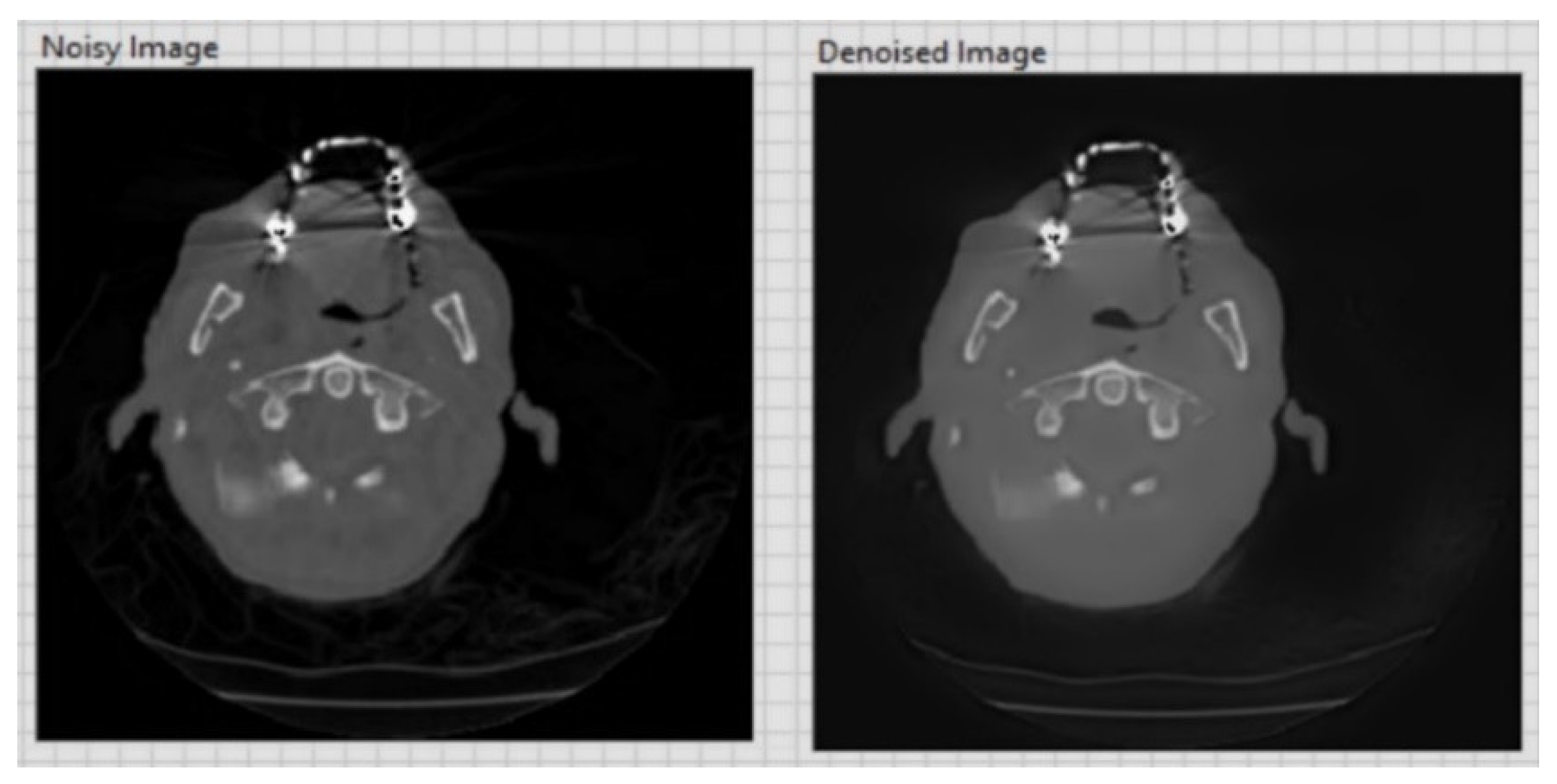
| CT image (Figure 6) 256 × 256 | 26.01 | 0.05 |
| CT image (Figure 7) 256 × 256 | 20.15 | 0.1 |
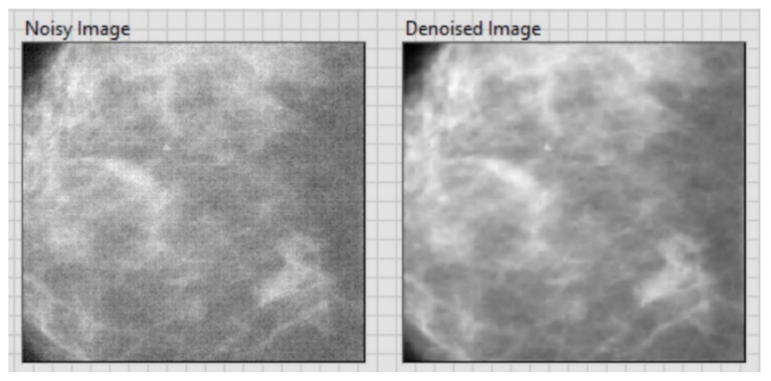
| CT image (Figure 8) 256 × 256 | 20.13 | 0.1 |
| CT image (Figure 9) 256 × 256 | 26.09 | 0.05 |
| CT image (Figure 10) 256 × 256 | 20.18 | 0.1 |
| CT image (Figure 11) 256 × 256 | 26.15 | 0.05 |
| By Adaptive Soft Truncation with Contextual Modeling (Chang) | By Applying the Simplified Algorithm, Based on Local Statistics | |||
|---|---|---|---|---|
| L | PSNR (dB) | C (%) | PSNR (dB) | C (%) |
| 3 | 28.98 | 64.74 | 30.00 | 67.14 |
| 5 | 28.99 | 65.31 | 29.99 | 67.08 |
| 10 | 29.02 | 64.74 | 29.90 | 66.82 |
| 20 | 29.21 | 63.85 | 29.81 | 65.73 |
| 50 | 29.31 | 64.53 | 29.76 | 66.20 |
| Image | Initial | Soft Truncation with Optimal Threshold Values | Soft Truncation with Local Statistics n = 3, L = 3 | Soft Truncation with Local Statistics n = 3, L = 5 | Soft Truncation with Local Statistics n = 3, L = 7 | Soft Truncation with Local Statistics n = 4, L = 3 | Soft Truncation with Local Statistics n = 4, L = 5 | ||||||||
|---|---|---|---|---|---|---|---|---|---|---|---|---|---|---|---|
| PSNR (dB) | C (%) | PSNR (dB) | C (%) | PSNR (dB) | C (%) | PSNR (dB) | C (%) | PSNR (dB) | C (%) | PSNR (dB) | C (%) | PSNR (dB) | C (%) | ||
| Lena | 0.05 | 26.00 | 63.94 | 29.74 | 61.96 | 30.27 | 65.84 | 30.18 | 65.51 | 30.08 | 65.75 | 30.27 | 65.67 | 30.18 | 65.48 |
| 0.1 | 20.06 | 48.10 | 26.13 | 44.65 | 26.59 | 46.74 | 26.57 | 45.66 | 26.49 | 46.38 | 26.01 | 46.78 | 26.59 | 45.80 | |
| Bridge | 0.05 | 26.09 | 63.59 | 27.49 | 62.67 | 27.65 | 62.56 | 27.65 | 62.74 | 27.65 | 62.76 | 27.65 | 62.36 | 27.65 | 62.86 |
| 0.1 | 20.13 | 48.07 | 23.38 | 44.76 | 23.45 | 43.75 | 23.48 | 44.03 | 23.49 | 43.87 | 23.45 | 43.99 | 23.48 | 43.96 | |
| House | 0.05 | 26.05 | 65.47 | 31.17 | 62.89 | 31.72 | 66.93 | 31.57 | 66.59 | 31.42 | 66.93 | 31.73 | 67.03 | 31.58 | 66.51 |
| 0.1 | 20.18 | 49.04 | 27.56 | 51.59 | 28.07 | 53.78 | 27.98 | 52.55 | 27.80 | 52.66 | 28.12 | 53.78 | 28.02 | 52.81 | |
| Boat | 0.05 | 26.03 | 64.03 | 30.44 | 62.72 | 30.87 | 65.06 | 30.74 | 64.75 | 30.66 | 65.22 | 30.87 | 65.00 | 30.75 | 64.92 |
| 0.1 | 20.03 | 47.09 | 26.83 | 46.12 | 27.10 | 49.53 | 27.08 | 48.16 | 27.00 | 47.75 | 27.14 | 49.92 | 27.11 | 49.22 | |
| Peppers | 0.05 | 26.04 | 63.50 | 30.08 | 60.78 | 30.44 | 62.36 | 30.32 | 63.44 | 30.22 | 63.36 | 30.43 | 62.40 | 30.32 | 63.40 |
| 0.1 | 20.16 | 50.88 | 26.51 | 48.65 | 26.78 | 49.28 | 26.73 | 49.28 | 26.66 | 48.47 | 26.79 | 49.30 | 26.74 | 49.12 | |
| Image | Initial Values | Processing Stage | Number of Wavelet Decomposition Levels N = 3 | Number of Wavelet Decomposition Levels N = 4 | ||
|---|---|---|---|---|---|---|
| PSNR (dB) | C (%) | PSNR (dB) | C (%) | |||
| Lena | PSNR = 26.00 dB C = 65.84% | After the second stage | 30.27 | 65.84 | 30.27 | 65.67 |
| Using the correlation map | 30.19 | 66.09 | 30.19 | 66.31 | ||
| Filtered correlation map | 30.22 | 65.98 | 30.23 | 66.23 | ||
PSNR = 26.00 dB C = 65.84% | After the second stage | 26.59 | 46.74 | 26.61 | 46.78 | |
| Using the correlation map | 26.29 | 48.17 | 26.30 | 47.99 | ||
| Filtered correlation map | 26.50 | 48.20 | 26.53 | 48.55 | ||
| Bridge | PSNR = 26.03 dB C = 62.96% | After the second stage | 27.59 | 61.26 | 27.59 | 61.15 |
| Using the correlation map | 27.54 | 62.83 | 27.53 | 62.96 | ||
| Filtered correlation map | 27.56 | 62.49 | 27.55 | 62.53 | ||
PSNR = 20.19 dB C = 47.44% | After the second stage | 23.48 | 44.66 | 23.49 | 44.81 | |
| Using the correlation map | 23.38 | 44.82 | 23.38 | 44.97 | ||
| Filtered correlation map | 23.46 | 44.49 | 23.47 | 44.76 | ||
| Aerial | PSNR = 26.06 dB C = 70.14% | After the second stage | 28.15 | 68.36 | 28.15 | 68.39 |
| Using the correlation map | 28.10 | 69.55 | 28.10 | 69.37 | ||
| Filtered correlation map | 28.13 | 69.39 | 28.12 | 69.29 | ||
PSNR = 20.15 dB C = 54.39% | After the second stage | 24.21 | 49.91 | 24.21 | 49.86 | |
| Using the correlation map | 24.07 | 52.75 | 24.06 | 53.13 | ||
| Filtered correlation map | 24.17 | 52.02 | 24.16 | 52.68 | ||
| Boat | PSNR = 26.03 dB C = 64.53% | After the second stage | 30.88 | 64.61 | 30.89 | 64.64 |
| Using the correlation map | 30.80 | 65.22 | 30.81 | 65.24 | ||
| Filtered correlation map | 30.84 | 64.75 | 30.85 | 64.92 | ||
PSNR = 20.07 dB C = 47.50% | After the second stage | 27.07 | 47.54 | 27.09 | 47.58 | |
| Using the correlation map | 26.72 | 48.84 | 26.72 | 49.43 | ||
| Filtered correlation map | 26.96 | 48.16 | 26.99 | 48.76 | ||
| House | PSNR = 26.05 dB C = 63.96% | After the second stage | 31.71 | 65.99 | 31.71 | 69.91 |
| Using the correlation map | 31.64 | 67.16 | 31.67 | 67.24 | ||
| Filtered correlation map | 31.67 | 66.82 | 31.70 | 66.95 | ||
PSNR = 20.10 dB C = 49.66% | After the second stage | 28.03 | 53.28 | 28.07 | 53.26 | |
| Using the correlation map | 27.66 | 53.85 | 27.69 | 54.32 | ||
| Filtered correlation map | 27.98 | 53.26 | 28.05 | 53.49 | ||
| Image | Initial | Method A (Integral Application of the Algorithm in Invariant Form to Translation) | Method B (Partial Application of the Algorithm in Invariant Form to Translation and Performing the Correction on This Result) | ||||||
|---|---|---|---|---|---|---|---|---|---|
| Average Results of Partial Travel Processing | After Performing the Correction Using the Contour Map | ||||||||
| PSNR (dB) | C (%) | PSNR (dB) | C (%) | PSNR (dB) | C (%) | PSNR (dB) | C (%) | ||
| Lena | 0.05 | 26.00 | 63.94 | 31.07 | 66.70 | 31.14 | 66.47 | 30.96 | 66.83 |
| 0.1 | 20.08 | 47.64 | 27.55 | 50.77 | 27.59 | 48.69 | 27.35 | 51.02 | |
| Bridge | 0.05 | 26.07 | 63.73 | 28.08 | 63.89 | 28.14 | 63.03 | 28.01 | 63.84 |
| 0.1 | 20.17 | 48.02 | 24.17 | 46.44 | 24.17 | 45.25 | 24.03 | 46.66 | |
| Aerial | 0.05 | 26.01 | 69.43 | 29.00 | 70.50 | 29.09 | 69.46 | 28.88 | 70.55 |
| 0.1 | 20.10 | 53.90 | 25.27 | 56.47 | 25.32 | 54.23 | 25.02 | 56.07 | |
| Boat | 0.05 | 26.03 | 64.12 | 31.97 | 67.28 | 32.03 | 67.18 | 31.82 | 67.18 |
| 0.1 | 20.03 | 47.58 | 28.19 | 51.26 | 28.25 | 50.15 | 27.94 | 51.12 | |
| House | 0.05 | 26.05 | 65.47 | 32.68 | 68.70 | 32.75 | 68.28 | 32.54 | 68.41 |
| 0.1 | 20.13 | 55.13 | 29.16 | 56.95 | 29.21 | 55.13 | 28.91 | 56.28 | |
| Image | Initial | Switched Type Correction | Continuous Type Correction | ||||
|---|---|---|---|---|---|---|---|
| PSNR (dB) | C (%) | PSNR (dB) | C (%) | PSNR (dB) | C (%) | ||
| Lena | 0.05 | 26.00 | 63.94 | 30.19 | 66.38 | 30.26 | 66.07 |
| 0.1 | 20.06 | 48.10 | 25.47 | 48.55 | 26.58 | 47.05 | |
| Bridge | 0.05 | 26.03 | 62.96 | 27.54 | 62.74 | 27.59 | 61.67 |
| 0.1 | 20.19 | 47.44 | 23.17 | 46.32 | 23.52 | 44.30 | |
| House | 0.05 | 26.05 | 65.47 | 31.66 | 67.55 | 31.72 | 67.40 |
| 0.1 | 20.14 | 50.96 | 26.49 | 55.08 | 28.00 | 53.59 | |
| Camera | 0.05 | 26.24 | 66.29 | 30.73 | 65.94 | 30.82 | 65.72 |
| 0.1 | 20.45 | 51.59 | 25.86 | 51.28 | 26.70 | 50.49 | |
| Boat | 0.05 | 26.03 | 64.03 | 30.80 | 65.84 | 30.86 | 65.66 |
| 0.1 | 20.00 | 45.78 | 25.63 | 48.92 | 27.00 | 47.27 | |
© 2020 by the authors. Licensee MDPI, Basel, Switzerland. This article is an open access article distributed under the terms and conditions of the Creative Commons Attribution (CC BY) license (http://creativecommons.org/licenses/by/4.0/).
Share and Cite
Simona Răboacă, M.; Dumitrescu, C.; Filote, C.; Manta, I. A New Adaptive Spatial Filtering Method in the Wavelet Domain for Medical Images. Appl. Sci. 2020, 10, 5693. https://doi.org/10.3390/app10165693
Simona Răboacă M, Dumitrescu C, Filote C, Manta I. A New Adaptive Spatial Filtering Method in the Wavelet Domain for Medical Images. Applied Sciences. 2020; 10(16):5693. https://doi.org/10.3390/app10165693
Chicago/Turabian StyleSimona Răboacă, Maria, Cătălin Dumitrescu, Constantin Filote, and Ioana Manta. 2020. "A New Adaptive Spatial Filtering Method in the Wavelet Domain for Medical Images" Applied Sciences 10, no. 16: 5693. https://doi.org/10.3390/app10165693
APA StyleSimona Răboacă, M., Dumitrescu, C., Filote, C., & Manta, I. (2020). A New Adaptive Spatial Filtering Method in the Wavelet Domain for Medical Images. Applied Sciences, 10(16), 5693. https://doi.org/10.3390/app10165693