Article

Decoding Visual Motions from EEG Using Attention-Based RNN

College of Intelligence Science and Technology, National University of Defense Technology, Changsha 410073, China
*
Author to whom correspondence should be addressed.
Appl. Sci. 2020, 10(16), 5662; https://doi.org/10.3390/app10165662
Submission received: 13 July 2020 / Revised: 8 August 2020 / Accepted: 11 August 2020 / Published: 14 August 2020
(This article belongs to the Special Issue Image Processing Techniques for Biomedical Applications)

Abstract

:
The main objective of this paper is to use deep neural networks to decode the electroencephalography (EEG) signals evoked when individuals perceive four types of motion stimuli (contraction, expansion, rotation, and translation). Methods for single-trial and multi-trial EEG classification are both investigated in this study. Attention mechanisms and a variant of recurrent neural networks (RNNs) are incorporated as the decoding model. Attention mechanisms emphasize task-related responses and reduce redundant information of EEG, whereas RNN learns feature representations for classification from the processed EEG data. To promote generalization of the decoding model, a novel online data augmentation method that randomly averages EEG sequences to generate artificial signals is proposed for single-trial EEG. For our dataset, the data augmentation method improves the accuracy of our model (based on RNN) and two benchmark models (based on convolutional neural networks) by 5.60%, 3.92%, and 3.02%, respectively. The attention-based RNN reaches mean accuracies of 67.18% for single-trial EEG decoding with data augmentation. When performing multi-trial EEG classification, the amount of training data decreases linearly after averaging, which may result in poor generalization. To address this deficiency, we devised three schemes to randomly combine data for network training. Accordingly, the results indicate that the proposed strategies effectively prevent overfitting and improve the correct classification rate compared with averaging EEG fixedly (by up to 19.20%). The highest accuracy of the three strategies for multi-trial EEG classification achieves 82.92%. The decoding performance for the methods proposed in this work indicates they have application potential in the brain–computer interface (BCI) system based on visual motion perception.

Graphical Abstract

1. Introduction

To build a direct communication pathway between the brain and environment, the brain–computer interface (BCI) based on electroencephalography (EEG) has been investigated for decades. It detects, analyzes, and decodes brain activities to translate them into commands for controlling external devices. The visual BCI that relies on external visual stimuli is a popular research direction in this field, owing to its robustness for different individuals and high information transfer rate (ITR) compared with motor imagery and spatial auditory BCI paradigms [1,2]. The most commonly used stimuli for the visual BCI are the flickering light or flipping of a static image, which evoke EEG signals such as P300 event-related potential (ERP) and steady-state visual evoked potential (SSVEP) [3,4,5]. To survive in a dynamic visual world, the human visual system is naturally sensitive to motion. That is, a video stimulus with motion events should be more likely to elicit enhanced brain activities and, therefore, has promise to be used to develop more effective BCI systems.
Although the perception of motion has been widely studied by neuroimaging and neurophysiology techniques such as fMRI, PET, and EEG [6,7,8], introducing it into the BCI system is a recent development. In some BCI systems for real-time monitoring and control, motion onset and periodic motion are utilized to evoke motion onset visual evoked potential (mVEP) and steady-state motion visual evoked potential (SSMVEP) signals transferring user intentions [9,10]. Surprisingly, most of the existing mVEP and SSMVEP paradigms only involve one motion mode. Although a few studies used contraction–expansion as stimulus [11,12,13], the contraction–expansion is taken as a periodic motion stimulus to evoke SSMVEP rather than two different motions. The visual responses for different motion types are not well utilized to increase the number of control commands for BCI. On the other hand, in some special BCI systems for motion event detection, preference identification and emotion recognition, dynamic videos depicting more motions are chosen as stimuli. However, all these works require long video clips (lasting for more than 5 s), which is not suitable for real-time applications.
To overcome the above deficiencies, in this study, short video clips (lasting for 1 s) illustrating four kinds of visual motions (contraction, expansion, rotation, and translation) are selected as stimuli. Previous research [8] demonstrates that the type of motion (translation, contraction, expansion, and rotation) affects the temporal and spatial features of EEG signals. They used grand average potentials obtained in the four motion types and source location analysis to reveal the differences among motions. However, the feasibility of decoding the type of above motions from single-trial EEG has not been investigated.
The classification accuracy of EEG signals is a key factor affecting the performance of BCI systems. EEG collected from the scalp is affected by brain background activity and artifacts like eyes blinks and electrooculogram, so its signal-to-noise ratio (SNR) is very low. Therefore, it is still challenging to classify EEG signals, especially when BCI uses stimuli with complex patterns. In the last few years, deep learning (DL) methods have been demonstrated to be effective in extracting motion-related events from the EEG [14,15,16]. Convolutional neural networks (CNNs) and recurrent neural networks (RNNs) are the two most frequently applied DL models.
RNNs are capable of capturing long-term dependencies in time sequences, and the context correlation of EEG reflected the type of stimulus [17,18]. In this study, we introduce attention mechanism into RNN as the decoding model. Attention mechanism has been widely used in natural language processing (NLP), based on the fact that words in a source sentence are not equally important to the target task. When applying the attention mechanism to a time sequence, varied emphases are placed on different parts of it, according to their significance. The attention mechanism is also applicable for EEG analysis, because samples in an EEG sequence are differentially informative. Existing studies utilizing attention-based RNN [16,19,20] for EEG analysis apply attention mechanisms to the hidden states of RNN. However, in the RNN architecture, the hidden state is updated recurrently at each time step, so those hidden states near the end are expected to capture more information, which may result in a biased attentive weight towards the later coming samples in RNN [21]. Consequently, the attention weights cannot reveal how relevant a specific part of the raw EEG signal is for the prediction result. This defect is called ‘attention bias’. In our framework, we add attention to the input EEG data before RNN computes the feature representation of EEG to avoid this problem. There are two advantages to this: First, attention can directly process the signal to suppress noise and emphasize task-relevant information in it, thereby promoting the neural network to extract more robust features of signals. Second, the weights learned by the attention mechanism can be visualized through a heatmap to increase the interpretability of the deep neural network.
Using DL to analyze EEG data is more challenging than to analyze images and audio. This is mainly because of two reasons. First, the number of samples in most EEG datasets is limited [22]. When the model is too complex, such as containing parameters that are much larger than the number of training samples, overfitting may occur, which will weaken its generalization ability. Second, the inter-trial and the inter-subject variabilities also affect the generalization ability of neural networks, because they cause inconsistencies between training data and test data. Generalization performance can be improved through data augmentation [23]. Many data augmentation techniques such as random cropping, noise addition, and affine/rotational distortions and unsupervised generative models (e.g., conditional GANs) have been applied to EEG [24,25,26,27]. The above methods increase the amount of EEG data, but do not consider the differences in SNR between trials.
During the EEG acquisition process, the physical and mental state of the subject fluctuates all the time, resulting in varying degrees of artifacts and neural background activities. Therefore, EEG data have various SNRs in different trials, and this variation exists even at different time periods within a trial. Such inter-trial difference undermines models’ generalization ability, leading to worse prediction accuracy. In this study, we propose a data augmentation approach that generates artificial signals by randomly averaging EEG data. In the EEG community, averaging is the most common method that changes SNR of EEG, based on the assumption that the task-unrelated brain activity is random noise [28]. Therefore, artificial signals with various SNR can be generated by averaging different numbers of EEG signals. The more SNR patterns included in the training data, the easier it is for the network to keep invariance to different levels of SNR in the test data. Notably, this data augmentation method is implemented during the training stage and, therefore, does not take up additional storage space.
The multi-trial EEG classification problem is also considered in this study. When more emphasis is placed on decoding accuracy and less on the real-time requirement, the BCI system performs the averaging for the ensemble of several signals before classification. This is a common practice in the P300 and mVEP BCI paradigms. However, the average potentials are generated in a fixed combination fashion (i.e., each trial is used only once), thus, reducing the number of training examples [29]. This may affect the generalization ability of the DL model and fail to achieve a better classification rate. To solve this problem, three strategies that randomly combine EEG are utilized for multi-trial EEG classification in this work. Compared with fixed combinations, random combinations allow the network to see more examples. They guarantee a noticeable increase in accuracy, even when the number of trials for combination is small.

2. Related Work

2.1. DL Methods for Classifying EEG Signals Evoked by Visual Stimuli

P300 and SSVEP are still the two most widely used signals in visual BCI systems because they only need simple and short duration stimuli. The two signals both have distinct features that are easy to extract. The video stimuli depicting motions could evoke EEG signals with more abstract and complicated features. Therefore, a review of the classification methods for EEG signals elicited by novel and long duration visual stimuli can inspire our work more. Baltatzis et al. [30] presented a signal decomposition method named swarm decomposition and a CNN to detect bullying incidences in EEG. Signals were recorded when subjects watched visual stimuli involving cases of bullying and non-bullying. Before being fed into CNN, the EEG signals were decomposed to several components, and the components that convey useless information were discarded. The findings show that SWD is a necessity for their CNN architecture to obtain reasonable classification rates. Behncke [31] et al. decoded erroneous robot behavior from the EEG of human observers using a deep CNN. The CNN obtained much higher classification accuracy than regularized linear discriminant analysis (rLDA). Teo et al. [32] used a deep neural network (DNN) to classify preferences (likes and dislikes) for 3D rotating visual stimuli from EEG. They achieved a classification performance better than those of other machine learning classifiers. Xing et al. [18] combined stack autoencoder (SAE) with RNN to recognize emotion induced by video stimuli. The SAE-based linear EEG mixing was used to decompose EEG signals to source signals and extract EEG channel correlations. The video lengths of the above studies varied from 5 s to 3 min. The effectiveness of deep learning for analyzing EEG evoked by informative video stimuli has been demonstrated.

2.2. Motion Stimuli for BCI Systems

Many studies have realized that motion can be an ideal stimulus for BCI systems. Guo et al. [9] utilized motion onset visual evoked potentials (mVEPs) for spelling, and the BCI application showed high accuracy and acceptable ITR compared to P300 ERP and SSVEP BCIs. Xie et al. [10] proposed a steady-state motion visual evoked potential (SSMVEP)-based BCI paradigm and proved that the paradigm could reduce users’ fatigue levels. Yan et al. [12] compared the accuracy and ITR of four SSMVEP paradigms based on basic motion modes: swing, rotation, spiral, and radial contraction–expansion. The results show that the spiral paradigm exhibited the highest average accuracy and ITR. The mVEP and SSMVEP paradigms have been widely used for BIC applications and have exhibited considerable comfort and stability [33,34]. However, only one motion mode was utilized in the above BCI systems.

2.3. Attention-Based RNNs

Bahdanau et al. [35] firstly extended the encoder–decoder with an attention mechanism for machine translation. The attention mechanism allows the model to detect the parts of a source sentence relevant to predicting a target word. Recently, some works introduced attention-based RNNs to EEG-related areas and achieved good results. Zhang et al. [20] proposed an attention-based encoder–decoder RNNs structure for person identification from EEG. The framework assigns various attention weights to different EEG channels based on the importance of each channel. Liu et al. [19] combined a Long Short-Term Memory (LSTM) network with temporal attention and band attention to recognize emotion from EEG. The EEG signals were transformed into a sequence of images on three frequency bands. The band attention assigned different weights to different frequency bands, while the temporal attention was applied to the hidden state of LSTM. Zhang et al. [16] also add temporal attention to hidden states of LSTM in a hand movement classification task with EEG. However, Wang et al. [21] noted that when adding the attention mechanism to hidden states, the attention bias problem may occur. They analyzed this problem in the answer selection task and found that words at the end of the sentence captured more attention.

2.4. Data Augmentation for EEG Signals

DL models contain a large number of learnable parameters, thus, requiring a significant amount of training data to optimize. Many recent works have investigated data augmentation methods for creating additional EEG data. Krell et al. [25] proposed a rotational data augmentation method for EEG data, similar to rotational distortions for image data augmentation. The approach increased the signal classification performance for BCI systems. Other image data augmentation methods, such as noise addition and random cropping, were also evaluated by the subsequent studies [24,26]. Some novel data augmentation methods were presented for EEG signals. Luo et al. [27] established a Conditional Wasserstein GAN (CWGAN) framework to generate augmented EEG data. Kalunga et al. [29] proposed an approach for augmenting EEG signals from their covariance matrices using Riemannian geometry.
In this paper, we will design a novel BCI paradigm based on motion perception and utilize an attention-based RNN to decode visual motions from EEG within one trial or a few trials. In contrast to the earlier BCI paradigms that utilize motion stimuli, we choose four types of video-depicted motions (contraction, expansion, rotation, and translation). The durations of the videos are only 1 s. Our attention-based RNN applies temporal attention directly to the raw EEG signals to the avoid attention bias problem, unlike the aforementioned attention-based RNN models. Besides, the input signals do not need any transformation, so our approach is simpler and more efficient. The online data augmentation proposed in this study generates artificial signals with different SNR during the model training. This method has not been considered and investigated in the above studies yet.

3. Materials

3.1. Participants

Eight healthy subjects participated in the study (mean age ± SD, 26.4 ± 3.7 years; one female and seven males). They were all volunteers from the National University of Defense Technology. Each subject showed normal or corrected to normal eyesight and no history of any neurological or psychiatric disorder. All participants provided written informed consent after receiving a comprehensive description of this study.

3.2. Experimental Protocol

Similar to the stimuli used in previous research [8], four types of motion were adopted in this experiment: translation (T), rotation (R), expansion (E), and contraction (C), all displayed on a gray (RGB: 96, 96, 96) background. The visual stimuli were made up of light gray (RGB: 136, 136, 136) and dark gray (RGB: 96, 96, 96) bands. They were presented on a 24-inch LCD monitor with a refresh rate of 60 Hz and a resolution of 1920 × 1080 pixels. The sizes of bright and dark bands of all stimuli were the same. Figure 1 shows the four stimuli displayed to the subjects.
The motion parameters of the stimuli were set as the same as that in [8], where the speed of T, E, and C was all set to 7.4 °/s and R stimulus was rotated at 40 rotations per minute. All stimuli had a viewing angle of 11.7° at a distance of 80 cm from the monitor. All motion animations were played at a frame rate of 45 fps. There were four blocks in the experiment, each with 8 runs. One run comprised 25 trials (i.e., 25 motion animations randomly chosen from the four types). The total duration of displaying a stimulus was 1000 ms, and the standard onset asynchrony (SOA) was 2000 ms. Thus, the inter-stimulus interval (ISI) was 1000 ms, in which the monitor displayed a gray blank. To maintain mental stability, the subjects were asked to rest for 60 s between each run and 20 min between each block. Figure 2 illustrates the timing structure of one block.
Therefore, a total of 800 trials was obtained from each subject, and the entire dataset contained 6400 trials (8 × 800). A perceptual discrimination task was added to the experiment: a target cue was randomly presented within approximately 10% of the stimulus intervals, and the next stimulus may or may not be consistent with the cue (probabilities for both were 0.5). A participant was required to respond as soon as possible when the stimulus was presented by pressing a button, with the left button implying consistency and the right button implying inconsistency. The time of pressing the button and the correct response rates were recorded. Before the experiment began, the subjects were informed of the detailed procedure of the experiment and trained how to respond using the button.

3.3. Data Acquisition

Brain waves were acquired using a BrainAmp Standard amplifier (Brain Products GmbH, Germany) following the international extended 10–20 standard system. Signals were recorded from 32 electrodes at positions O1, Oz, O2, PO7, PO3, POz, PO4, PO8, P7, P5, P3, P1, Pz, P2, P4, P6, P8, TP9, CP5, CP1, CP2, CP6, TP10, T7, C5, C3, C1, CZ, C2, C4, C6, and T8, which ideally covered the dorsal pathway [36] involved with motion perception. The reference electrode was placed at Cz and the ground at AFz, so the number of signal channels was 31 (32–1). All electrode impedances were reduced to 10 kΩ before data acquisition. EEG signals were sampled at 500 Hz and filtered by a 0.1–100 Hz bandpass filter and a 50 Hz notch filter. Stimuli presentation and data collection were performed by the BCI2000 framework [37].

3.4. Data Preprocessing

The continuous EEG data were first visually inspected and trials severely contaminated by noises were removed. The signals were, then, passed through a 12–65 Hz zero phase shift filter to preserve the beta and the gamma bands associated with visual cognition [38]. In this way, the effect of ocular artifacts was also reduced [39]. The clean raw data plugin in EEGLAB toolbox [40] was applied to remove low-frequency drifts, noisy channels, and short-time bursts from the data. The removed channels were replaced through the spherical interpolation method implemented in EEGLAB. Finally, the number of signals in each category was balanced for further analysis. In the end, a total of 6000 (1500 × 4) trials were retained. All trial channels were additionally normalized between −1 and 1, with a mean of zero. For each EEG recording, the first 50 samples were excluded to reduce the interference of inter-stimulus intervals.

4. Methods

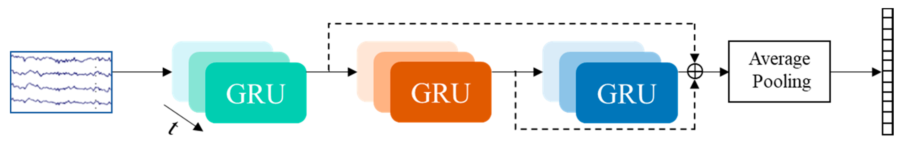
4.1. Stacked GRU with Skip Connections

Gated Recurrent Unit (GRU) [41], one of the two commonly used RNN variants, is exploited in this study because it not only addresses the gradient vanishing problem associated with RNN but also is more lightweight than the other variant, namely LSTM [42]. Compared with LSTM, GRU has a better generalization on smaller datasets, and it is easier to train. GRU can be formulated as follows:
z t = σ ( W z x t + U z h t 1 ) r t = σ ( W r x t + U r h t 1 ) h ˜ t = tanh ( W x t + U ( r t h t 1 ) ) h t = ( 1 z t ) h t 1 + z t h ˜ t
where x t and h t 1 are the input and output of GRU at time t; W z , W r , U z , and U r are weight matrices and stands for element-wise multiplication. GRU units are stacked to improve the mining of temporal correlations. Skip connections are introduced in our framework to pass the output of different layers of stacked GRU directly to the classification layer. This way, the classification layer receives a combination of low-level and high-level features. Skip connections allow better information and gradient flow, thus, making the network easier to optimize [43,44]. They also solve the degradation problem caused by the increased depth of the neural network. The skip connection in this study is similar to that of DenseNet [44]: it combines features through concatenation rather than summation. The k-layer stacked GRU with skip connections (SC-GRU) can be expressed as follows:
h t ( j ) = G ( h t ( j ) + h t ( j 1 ) ) h ˜ t = [ h t ( 1 ) ; h t ( 2 ) ; ; h t ( k ) ] r = t = 1 T h ˜ t T
where G is the GRU mapping, which converts the input to the GRU state, h t ( j ) is the state of the layer j at time t, h ˜ t is the concatenation of h t from layer 1 to layer k, and r is the EEG representation used for classification. The EEG representations carrying different categorical information are obtained by averaging h t of all-time steps (in our framework, a 1D global average pooling layer [45] is applied to calculate the averages). A fully connected layer for classification receives EEG representations nonlinearized by ReLU. The framework for the 3-layer SC-GRU is presented in Figure 3.

4.2. Attention-Based GRU

The attention mechanism is implemented through a fully connected layer jointly trained with GRU. The attention layer (AL) projects the input into a weight vector of equal length to the time dimension of the input. To compare the effect of the attention layer’s location, AL is placed before and after the GRU, respectively. The former puts attention on EEG signals, while the latter puts attention on EEG representations. Given a signal I containing T samples, then, I C   ×   T , where C is the number of channels of the EEG, and T is the length of the EEG sequence. The AL-GRU that puts AL before GRU can then be expressed as the following equations:
α t = σ ( W i t ) i ˜ t = α t i t h t = G ( i ˜ t , h t 1 ) r = t = 1 T h t T
While the GRU-AL that puts AL after GRU can be formulated as follows:
h t = G ( i t , h t 1 ) α t = σ ( W h t ) h ˜ t = α t h t r = t = 1 T h ˜ t T
where i t is the sample of the input EEG signal at time t, W is the weight matrix derived from back propagation with a dimension of C, α t is the attention weight, σ is sigmoid function that normalizes the weight between 0 and 1, and r is the EEG representation. In the experiment, AL-GRU and GRU-AL are also stacked, and skip connections are added to the framework.

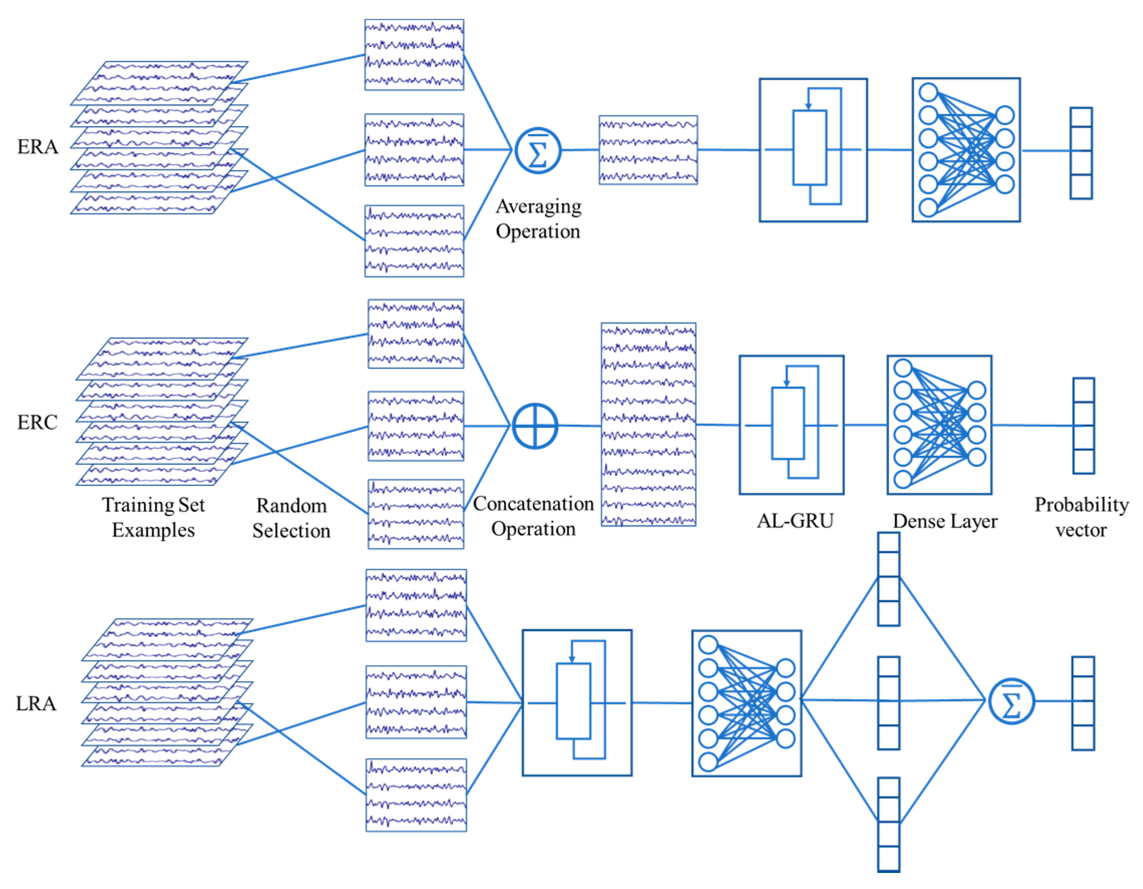
4.3. Data Augmentation by Randomly Averaging

During the model training, n examples are randomly taken from the same category to calculate the average potential at each iteration, where n is any integer between 1 and N. When n > 1, the average potential is considered as a new artificial sample for the model. N is the maximum number of signals needed to generate an artificial sample. A small N means that the data augmentation method adds insufficient diversity of SNR to the dataset. In contrast, a large N means the augmentation method may produce meaningless artificial data with unrealistic SNR. Too large N not only increases the training time but may also dilute the effect of network learning. We test the effect of different N values on the classification accuracy through experiments and determined the appropriate N for models.
To figure out whether the improvement in network performance is due to more than just an increase in the size of the dataset, a controlled experiment is performed by adding Gaussian noise to augment training samples. Adding Gaussian noise is a simple data augmentation method that works well when the amount of data is much less than the model parameters (e.g., MAHNOB-HCI [46] dataset vs. ResNet [43]). The mean of the Gaussian noise is set to 0 to keep the signals’ amplitudes unchanged. For each training iteration, a value from 0, 0.04, 0.08, 0.12, 0.16, and 0.2 is randomly chosen as the standard deviation of Gaussian noise (0 means no noise is added), since it has been demonstrated that the standard deviations between 0.01 and 0.2 works better [24]. Random averaging is an online data augmentation method that utilizes the iterative training property of neural networks. There is no need to augment data before the training. Instead, new samples are continuously generated before each training iteration for the network to configure its weights and biases, thus, saving storage space and time.

4.4. Multi-Trial Combination Strategies

For multi-trial EEG decoding, three combination strategies for training examples are proposed in this paper: early randomly averaging (ERA), early random concatenation (ERC), and late randomly averaging (LRA). ERA averages several EEG signals randomly taken from one category at each training iteration. ERC on its part concatenates the signals along the channel dimension, inspired by genetic recombination in sexual reproduction. One possible explanation for the superiority of sexual reproduction is that, over the long term, the criterion for natural selection may not be individual fitness but rather mixability of genes [47]. Given a single-trial signal I C × T , where C is the number of signal channels, and T is the length of the EEG sequence, after combining k trials according to the ERC, multi-trial signal I E R C ( k C ) × T is obtained. LRA randomly averages the probability vectors output by the classifier. This approach adds diversity to the output and reduces the likelihood of false predictions by averaging the predictions of different trials. Under the ideal condition (sufficient training time for the model), the number of samples generated by the three strategies is C (n, k), P (n, k), and C (n, k), where n is the number of training samples, C (n, k) is k-combinations of n, and P (n, k) is k-permutations of n. Note that all randomly combining methods are for the training set examples during the training stage and the test set examples are generated in a fixed combining manner (i.e., all single-trial EEG signals are combined only once). The procedure for the three combination schemes is described in Figure 4.

4.5. Model Configuration and Training

Layer normalization [48] is added before each layer of stacked GRU and applied over the channel dimensions of the input signal to speed up convergence and improve performance. Based on our pre-experimental results, layer normalization can effectively improve model performance, and it is better to place before GRU than after GRU. Dropout [47] is added to non-recurrent connections to prevent overfitting, whereas the early stopping method is adopted to achieve optimal generalization performance. RAdam optimizer is used as the loss function optimization algorithm, with a learning rate of 0.001 [49]. The optimizer ensured a comparable or even better performance without warm-up for the learning rate. Xavier initialization [50] and Kaiming initialization [51] are adopted to initialize the parameters of GRU and the fully connected layer, respectively. The model is trained by minimizing the cross-entropy loss:
L o s s ( O , L ) = i = 1 N log ( o i ) l i
where O is the probability vector normalized by the softmax function with a dimension of N, N is the number of signal categories, and L is the one-hot vector of the true label of signals. All models used in this study were built in PyTorch [52] and trained on an NVIDIA GEFORCE RTX 2080 Ti GPU.

4.6. Model Configuration and Training

EEGNet and DeepConvNet [26,53], two prevalent CNN-based structures for decoding EEG, are selected for comparison. EEGNet is an EEG-specific network that incorporates EEG feature extraction concepts and contains comparatively less trainable parameters. The EEGNet-8,2 model, a version of EEGNet that performs well on almost all the EEG classification tasks, is used in the experiment. DeepConvNet is a generic architecture to extract a wide range of features from EEG inspired by successful approaches in computer vision. On the basis of the original framework of EEGNet-8,2, the last average pooling layer is replaced with the global average pooling type to reduce the parameters, and the dropout layer is removed. This minimizes the disharmony between dropout and batch normalization [54]. In fact, both batch normalization and global average pooling have regularization properties, and some successful architectures, such as ResNet and DenseNet, achieve their best performance without dropouts through the application of these techniques. In our pre-experiments, we find the performance of EEGNet-8,2 to be better and more stable after the replacement.

5. Results and Discussion

5.1. Reaction Times for Each Motion

The overall proportion of correct responses is 95.12%. One-way ANOVA and multiple comparison tests with a Bonferroni post hoc correction are performed to analyze the differences among reaction times (RTs) for each motion. The corresponding reaction times and p-values of statistical tests are shown in Table 1. The results indicate that there is no significant effect of motions on RTs (F (3, 627) = 2.247, p = 0.082).

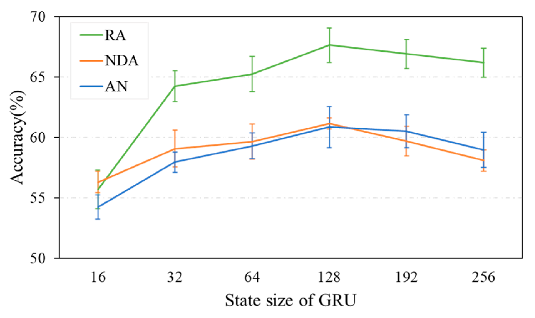
5.2. Performance of Attention-Based GRU with Skip Connections

Five-fold cross-validation is used to obtain the final classification results of the dataset that contained 6000 trials. To make sure that the attention layers for AL-GRU and GRU-AL have the same size, the state size of GRU is set to 31, consistent with the number of signal channels. Table 2 shows the decoding accuracies of the attention-based GRU with skip connections for different numbers of stacked layers. The performance of GRU improves after the addition of skip connections, which alleviates the degradation caused by the increase in network depth. AL-GRU achieves the best classification rate of 61.74% when the number of stacked layers is four, better than that obtained in EEGNet-8,2, but worse than that obtained in DeepConvNet.
The parameters numbers for these three structures are 2.4k, 28.5k, and 184.5k, respectively. It seems that DeepConvNet has obvious superiority due to its complex structure and the larger parameter amount. The attention mechanism boosts the performance of GRU, especially when there are few stacked layers. This may be because the attention mechanism improves the limited feature extraction ability of the shallow network, so that it can learn high-level features which are more robust among trials. The confusion matrices of AL-GRU, EEGNet-8,4, and DeepConvNet are shown in Figure 5.
The confusion pattern from the confusion matrix for the single-trial EEG classification is apparent. The model is prone to misprediction between contraction and expansion and between rotation and translation. The recall for a category less than 50% suggests that the model tends to mistake it for the other similar category. For example, the recall of DeepConvNet for contraction is 39.40%, with more than half of the contraction examples being incorrectly predicted as expansion. The performance of the models needs to be further improved.

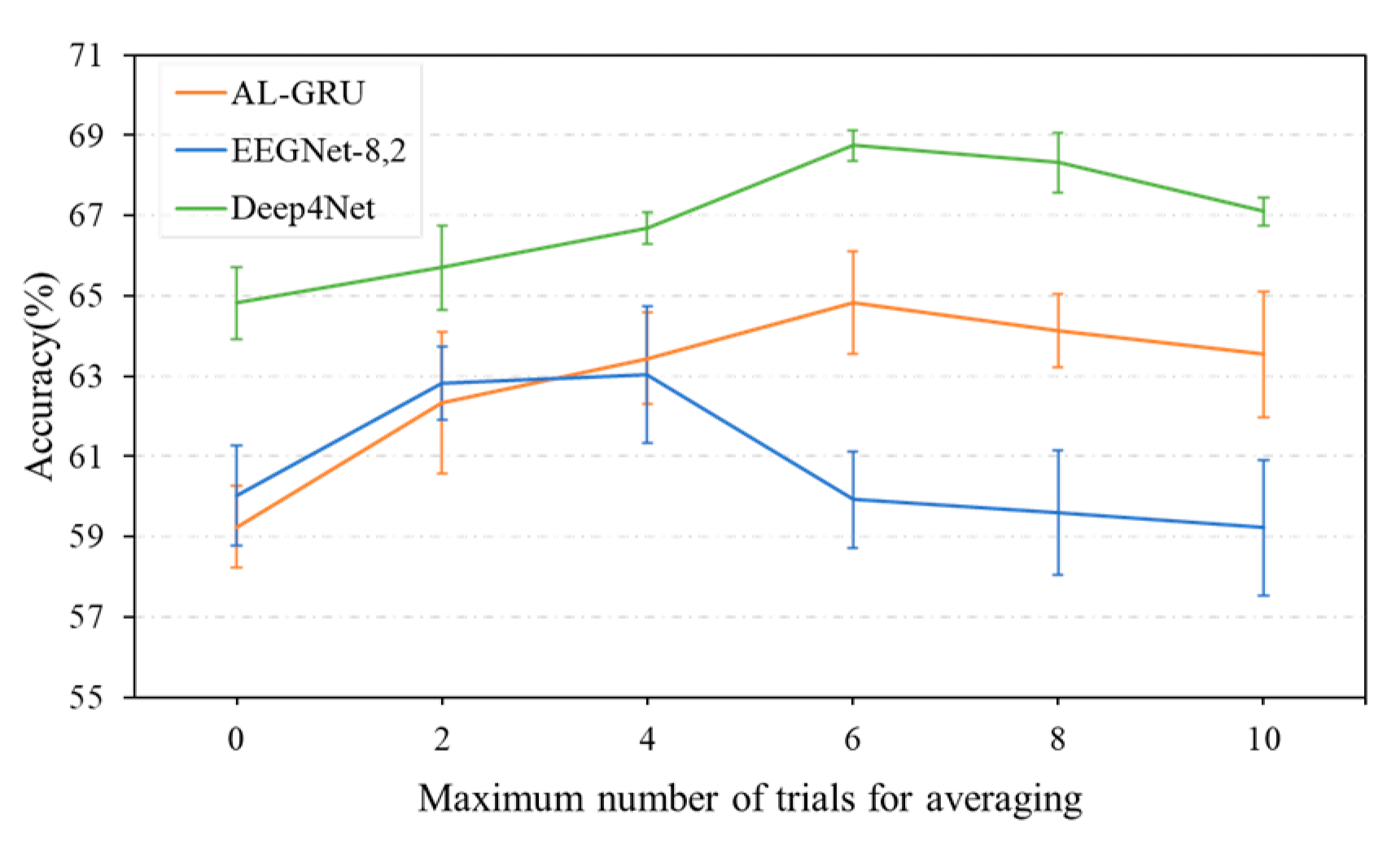
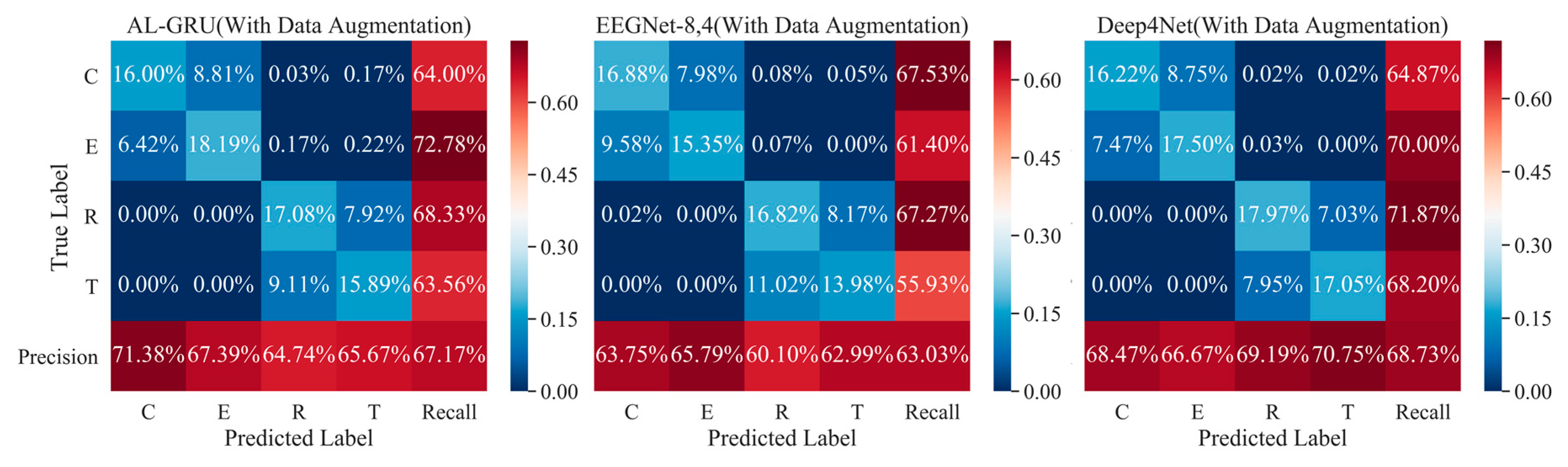
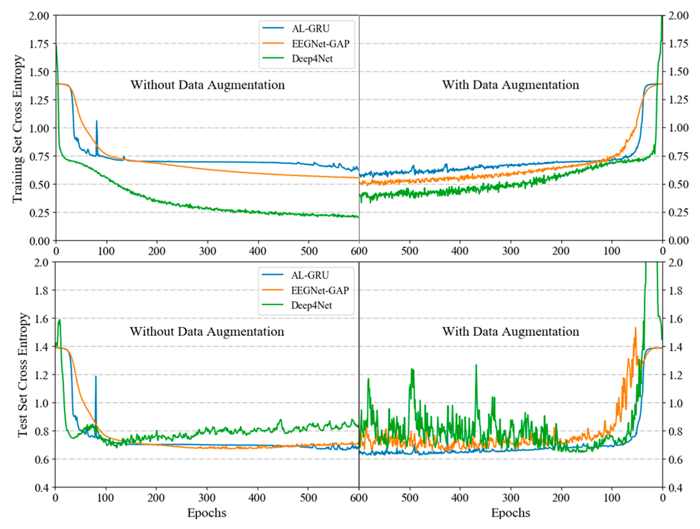
5.3. Performance of Data Augmentation by Randomly Averaging

Since the purpose of this experiment is to study the effect of the proposed data augmentation method, we adopt the single-layer AL-GRU structure that is easy to optimize. The state size of the GRU is set to 31. EEGNet-8,2 and DeepConvNet are also used for comparison. The effect of the maximum number of trials for averaging (N) on the network performance is shown in Figure 6. Compared with non-augmentation, our method shows obvious advantages. It improves the accuracies of AL-GRU, DeepConvNet, and EEGNet-8,2 by 5.60%, 3.92%, and 3.02%, respectively. AL-GRU and DeepConvNet show the best performance when N is 6, while EEGNet-8,2 obtains the highest accuracy when N is 4. AL-GRU benefits more from this approach. However, the improvement of EEGNet-8,2 is limited, which may due to the smaller size of the model. The data augmentation method allows the networks to see more data with different SNR, thus, improving generalization performance on unseen data.
Figure 7 shows the comparison of decoding accuracies among randomly averaging, the addition of Gaussian white noise, and non-augmentation. N is set to 6, and the AL-GRU state size that determines the number of parameters varies from 16 to 256. Here, as the state size increases, the test accuracies improve at first, until too many model parameters result in overfitting. Compared with non-augmentation, randomly averaging can consistently improve the accuracy regardless of the state size of GRU, while adding noise to the data cannot. The reason may be that adding noise does not provide any new information to signals but only increases the number of training samples. The volume of data used in this research is favorably large. When the model is not excessively complex, the addition of noise may not bring a significant improvement. Data augmentation by randomly averaging incorporates information about the change in SNR, thus, promoting the performances of the networks with different complexity. The highest accuracy is 67.18% when the state size of AL-GRU is 128.
The confusion matrices of the models at their best performance are presented in Figure 8. The recalls of the models have also been improved. This indicates that the augmented data helps the models learn high-level features, so as to better distinguish signals of similar categories.
Optimization learning curves for models over 600 epochs can be seen in Figure 9. The learning curve of the training set reflects how well the model is learning, while the learning curve of the test set gives an idea of how well the model is generalizing. Compared with non-augmentation, randomly averaging reduces cross-entropy losses for both test and training sets of AL-GRU and EEGNet-8,2.
However, it is interesting to observe that for DeepConvNet, only the loss of the test set decreases. One possible explanation for this discrepancy is that for the complex network (e.g., DeepConvNet) with strong learning ability, data augmentation makes it less specialized for training data to obtain a better generalization performance. In contrast, for the shallow networks (e.g., AL-GRU and EEGNet-8,2), the augmented data with useful features enhance their poor fitting capabilities. Thus, both the learning and generalization performance improves. The learning curves of test set for the CNN-based networks are more unstable than that of AL-GRU. This may be because the data augmentation method adds new examples to each mini-batch, and the batch normalization layer is sensitive to data distribution changes [55].

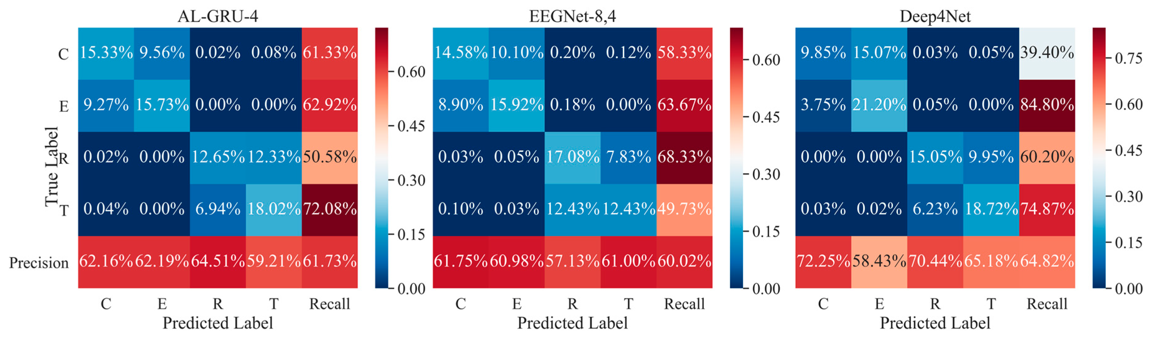
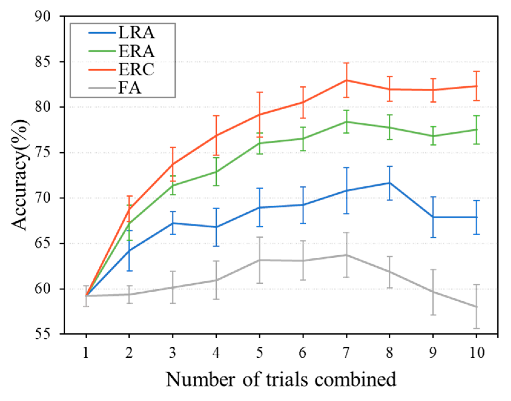
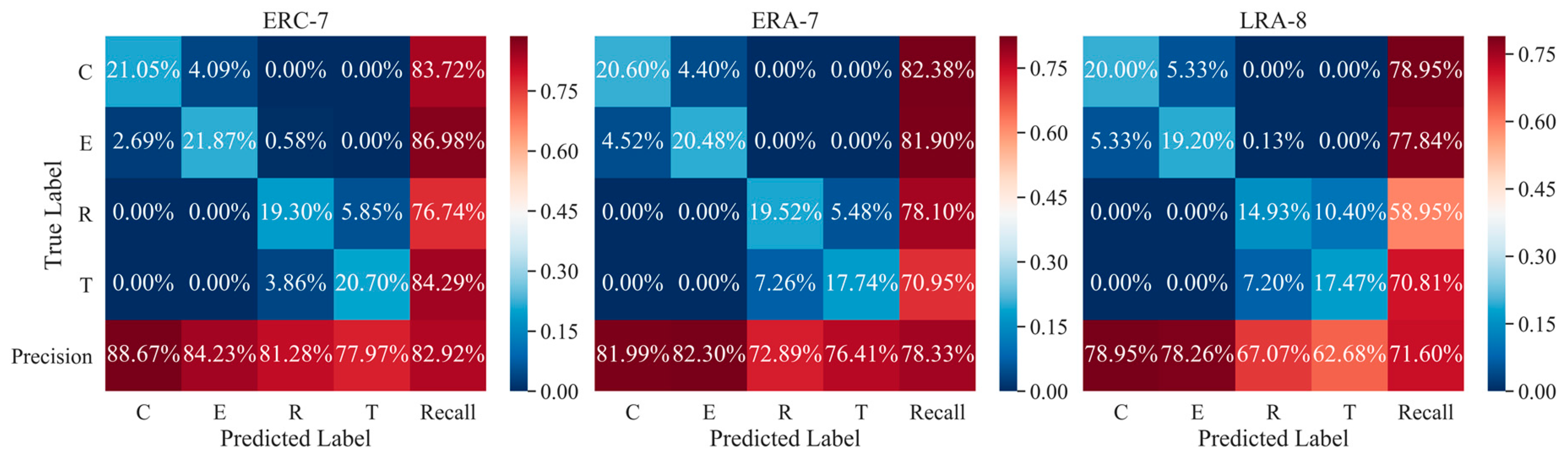
5.4. Performance of Combination Strategies for Multi-Trial EEG Decoding

AL-GRU with a state size of 128 is used in this experiment. The decoding accuracies of different random combination strategies and the fixed averaging scheme used in traditional ERP analyses are given in Figure 10. Here, fixed averaging does not bring a significant increase for accuracy. In fact, the accuracy starts to decline when the number of averaged trials is more than seven. This implies that the gains from increasing SNR are no longer sufficient to counteract the overfitting caused by the decrease in the volume of the data. The random combination strategies are designed to solve problems related to sample size reduction. ERC is the best strategy for such problems, shown to achieve the best accuracy of 82.92% when the number of trials combined is seven and accuracy of 73.72% when the number of trials combined is three.
Due to inter-trial variability, averaging data across trials may distort the waveforms and result in a loss of information [56]. The ERC strategy concatenates rather than averages different trials, thus, fully preserves information on the combined trials. This strategy provides more examples (P (n, k) > C (n, k)), also a strength that allows it to outperform ERA. The LRA strategy increases the diversity of the output rather than input, so it is inferior to the other strategies. Confusion matrices of the combination strategies at their best performance are shown in Figure 11.

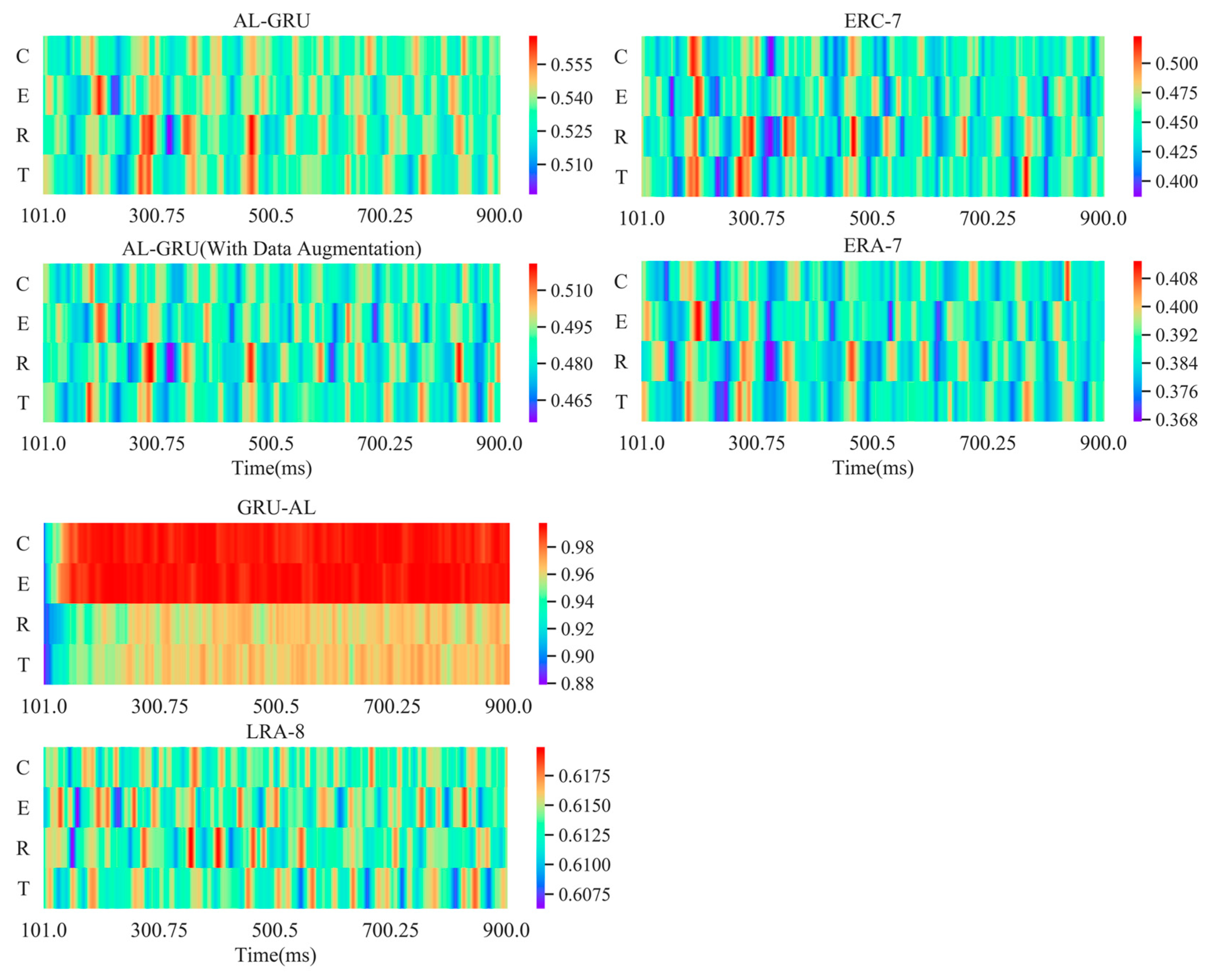
5.5. Attention Weights Visualization

Figure 12 visualizes the attention weights of the four motions (C, E, R, and T) under different models and combination strategies. The attention weights used here are averages of attention weights of all EEG signals when the model training is completed. The larger the weight is, the more attention the model pays to the corresponding part of the time sequence. Here, the attention bias problem can be observed in GRU-AL (i.e., more attention is allocated to the posterior part of the EEG representation), while the attention distribution of AL-GRU is more uniform.
After the data augmentation and combining multiple trials through ERC and ERA, more attention is focused on fewer parts of the signal. This indicates that the data augmentation method and combination strategies proposed in this study make it easier for the model to extract robust features among different trials. Unlike the other two strategies, the attention of LRA is distributed in various time periods. The focus on irrelevant features explains the poor performance of LRA. The weight ranges for ERC, ERA, and LRA are between [0.370, 0.540], [0.367, 0.412], and [0.606,0.620], respectively. The greater the difference between the maximum and minimum weight, the more confident the model is in feature selection. ERC owning the largest weight range shows that it can better improve signal quality after combination compared to other strategies.
According to the weight distribution of ERC-7 and ERA-7 over time, it can be deduced that attention is not only paid to time periods around 200 ms containing the N2 component related to motion perception [9,57], but also to other time periods of the signal. The DL model not only learns the handcrafted features commonly used in traditional EEG analysis but also incorporates other abstract features.

6. Conclusions

In this study, an attention-based GRU is utilized to decode motion types from EEG data. To our best knowledge, this is the first attempt to introduce the four movements of contraction, expansion, rotation, and translation as visual stimuli into BCI applications. Unlike the previous research using attention-based RNN to analyze EEG, an attention mechanism is applied to raw EEG data, which not only improves the classification performance but also increases the interpretability of the model. This work implies the attention mechanism can be used for EEG preprocessing and analysis.
The data augmentation method proposed in this work generates artificial examples with different SNRs through randomly averaging EEG signals. This method offers the decoding model better generalization ability and robustness to SNR variabilities. Besides, it is performed during the model training, which saves storage space and is easy to extend to other existing DL models.
As for multi-trial classification, ERC randomly concatenates the signals to generate more training examples and performs best among all strategies. After a combination of three trials, the accuracy for division into four classes achieves 73.72%, which demonstrates the potential of this method to be applied to BCI systems with strict real-time requirements.

Author Contributions

Methodology, D.Y.; Software, D.Y.; Validation, Y.Y. and Z.Z.; Formal analysis, Y.L. and X.L.; Writing—original draft preparation, D.Y.; Writing—review and editing, Y.L. All authors have read and agreed to the published version of the manuscript.

Funding

This research was supported by the National Natural Science Foundation of China (Grants No. U19A2083).

Conflicts of Interest

The authors declare no conflict of interest. The funders had no role in the design of the study; in the collection, analyses, or interpretation of data; in the writing of the manuscript, or in the decision to publish the results.

References

  1. Padfield, N.; Zabalza, J.; Zhao, H.; Masero, V.; Ren, J. EEG-Based Brain-Computer Interfaces Using Motor-Imagery: Techniques and Challenges. Sensers 2019, 19, 1423. [Google Scholar] [CrossRef] [PubMed] [Green Version]
  2. Schreuder, M.; Blankertz, B.; Tangermann, M. A New Auditory Multi-Class Brain-Computer Interface Paradigm: Spatial Hearing as an Informative Cue. PLoS ONE 2010, 5, e9813. [Google Scholar] [CrossRef] [PubMed]
  3. Fazel-Rezai, R.; Allison, B.Z.; Guger, C.; Sellers, E.W.; Kleih, S.C.; Kübler, A. P300 brain computer interface: Current challenges and emerging trends. Front. Neuroeng. 2012, 5, 14. [Google Scholar] [CrossRef] [PubMed] [Green Version]
  4. Chen, Y.-J.; Chen, S.-C.; Zaeni, I.A.E.; Wu, C.-M. Fuzzy Tracking and Control Algorithm for an SSVEP-Based BCI System. Appl. Sci. 2016, 6, 270. [Google Scholar] [CrossRef] [Green Version]
  5. Liu, Y.-H.; Wang, S.-H.; Hu, M.-R. A Self-Paced P300 Healthcare Brain-Computer Interface System with SSVEP-Based Switching Control and Kernel FDA + SVM-Based Detector. Appl. Sci. 2016, 6, 142. [Google Scholar] [CrossRef] [Green Version]
  6. Morrone, M.C.; Tosetti, M.; Montanaro, D.; Fiorentini, A.; Cioni, G.; Burr, D.C. A cortical area that responds specifically to optic flow, revealed by fMRI. Nat. Neurosci. 2000, 3, 1322–1328. [Google Scholar] [CrossRef]
  7. McKeefry, D.J.; Watson, J.D.; Frackowiak, R.S.; Fong, K.; Zeki, S. The activity in human areas V1/V2, V3, and V5 during the perception of coherent and incoherent motion. Neuroimage 1997, 5, 1–12. [Google Scholar] [CrossRef]
  8. Delon-Martin, C.; Gobbelé, R.; Buchner, H.; Haug, B.A.; Antal, A.; Darvas, F.; Paulus, W. Temporal pattern of source activities evoked by different types of motion onset stimuli. Neuroimage 2006, 31, 1567–1579. [Google Scholar] [CrossRef]
  9. Hong, B.; Guo, F.; Liu, T.; Gao, X.; Gao, S. N200-speller using motion-onset visual response. Clin. Neurophysiol. 2009, 120, 1658–1666. [Google Scholar] [CrossRef]
  10. Xie, J.; Xu, G.; Wang, J.; Li, M.; Han, C.; Jia, Y. Effects of Mental Load and Fatigue on Steady-State Evoked Potential Based Brain Computer Interface Tasks: A Comparison of Periodic Flickering and Motion-Reversal Based Visual Attention. PLoS ONE 2016, 11, e0163426. [Google Scholar] [CrossRef]
  11. Gao, Z.; Yuan, T.; Zhou, X.; Ma, C.; Ma, K.; Hui, P. A Deep Learning Method for Improving the Classification Accuracy of SSMVEP-based BCI. IEEE Trans. Circuits Syst. Ii Express Briefs 2020. [Google Scholar] [CrossRef]
  12. Yan, W.; Xu, G.; Xie, J.; Li, M.; Dan, Z. Four Novel Motion Paradigms Based on Steady-State Motion Visual Evoked Potential. IEEE Trans. Biomed. Eng. 2018, 65, 1696–1704. [Google Scholar] [CrossRef] [PubMed]
  13. Park, S.; Cha, H.; Im, C. Development of an Online Home Appliance Control System Using Augmented Reality and an SSVEP-Based Brain–Computer Interface. IEEE Access 2019, 7, 163604–163614. [Google Scholar] [CrossRef]
  14. Ma, T.; Li, H.; Yang, H.; Lv, X.; Li, P.; Liu, T.; Yao, D.; Xu, P. The extraction of motion-onset VEP BCI features based on deep learning and compressed sensing. J. Neurosci. Methods 2017, 275, 80–92. [Google Scholar] [CrossRef]
  15. Carvalho, S.R.; Filho, I.C.; Resende, D.O.D.; Siravenha, A.C.; Souza, C.R.B.D.; Debarba, H.; Gomes, B.D.; Boulic, R. A Deep Learning Approach for Classification of Reaching Targets from EEG Images. In Proceedings of the 2017 30th SIBGRAPI Conference on Graphics, Patterns and Images (SIBGRAPI), Niterói, Brazil, 17–20 October 2017; pp. 178–184. [Google Scholar]
  16. Zhang, G.; Davoodnia, V.; Sepas-Moghaddam, A.; Zhang, Y.; Etemad, A. Classification of Hand Movements From EEG Using a Deep Attention-Based LSTM Network. IEEE Sens. J. 2020, 20, 3113–3122. [Google Scholar] [CrossRef] [Green Version]
  17. Roy, Y.; Banville, H.; Albuquerque, I.; Gramfort, A.; Falk, T.H.; Faubert, J. Deep learning-based electroencephalography analysis: A systematic review. J. Neural Eng. 2019, 16. [Google Scholar] [CrossRef]
  18. Xing, X.; Li, Z.; Xu, T.; Shu, L.; Hue, B.; Xu, X. SAE plus LSTM: A New Framework for Emotion Recognition From Multi-Channel EEG. Front. Neurorobotics 2019, 13. [Google Scholar] [CrossRef]
  19. Liu, J.; Su, Y.; Liu, Y. Multi-modal Emotion Recognition with Temporal-Band Attention Based on LSTM-RNN. In Advances in Multimedia Information Processing-Pcm 2017, Pt I; Zeng, B., Huang, Q., ElSaddik, A., Li, H., Jiang, S., Fan, X., Eds.; Springer: Cham, Switzerland, 2018; Volume 10735, pp. 194–204. [Google Scholar]
  20. Zhang, X.; Yao, L.; Kanhere, S.S.; Liu, Y.; Gu, T.; Chen, K. MindID: Person Identification from Brain Waves through Attention-based Recurrent Neural Network. Proc. Acm Interact. Mob. Wearable Ubiquitous Technol. 2018, 2, 149. [Google Scholar] [CrossRef]
  21. Wang, B.; Liu, K.; Zhao, J. Inner Attention based Recurrent Neural Networks for Answer Selection. In Proceedings of the 54th Annual Meeting of the Association for Computational Linguistics (Volume 1: Long Papers), Berlin, Germany, 7–12 August 2016; ACL: Beijing, China, 2016; pp. 1288–1297. [Google Scholar]
  22. Bashivan, P.; Rish, I.; Yeasin, M.; Codella, N. Learning representations from EEG with deep recurrent-convolutional neural networks. arXiv 2015, arXiv:1511.06448. [Google Scholar]
  23. Arvidsson, I.; Overgaard, N.C.; Åström, K.; Heyden, A. Comparison of Different Augmentation Techniques for Improved Generalization Performance for Gleason Grading. In Proceedings of the 2019 IEEE 16th International Symposium on Biomedical Imaging (ISBI 2019), Venice, Italy, 8–11 April 2019; pp. 923–927. [Google Scholar]
  24. Wang, F.; Zhong, S.-h.; Peng, J.; Jiang, J.; Liu, Y. Data Augmentation for EEG-Based Emotion Recognition with Deep Convolutional Neural Networks. In Multimedia Modeling, Mmm 2018, Pt Ii; Schoeffmann, K., Chalidabhongse, T.H., Ngo, C.W., Aramvith, S., Oconnor, N.E., Ho, Y.S., Gabbou, M., Elgammal, A., Eds.; Springer: Cham, Switzerland, 2018; Volume 10705, pp. 82–93. [Google Scholar]
  25. Krell, M.M.; Kim, S.K.; IEEE. Rotational Data Augmentation for Electroencephalographic Data. In Proceedings of the 2017 39th Annual International Conference of the IEEE Engineering in Medicine and Biology Society, Seogwipo, Korea, 11–15 July 2017; pp. 471–474. [Google Scholar]
  26. Schirrmeister, R.T.; Springenberg, J.T.; Fiederer, L.D.J.; Glasstetter, M.; Eggensperger, K.; Tangermann, M.; Hutter, F.; Burgard, W.; Ball, T. Deep Learning With Convolutional Neural Networks for EEG Decoding and Visualization. Hum. Brain Mapp. 2017, 38, 5391–5420. [Google Scholar] [CrossRef] [Green Version]
  27. Luo, Y.; Lu, B.-L. EEG Data Augmentation for Emotion Recognition Using a Conditional Wasserstein GAN. In Proceedings of the 2018 40th Annual International Conference of the IEEE Engineering in Medicine and Biology Society (EMBC), Honolulu, HI, USA, 18–21 July 2018; Volume 2018, pp. 2535–2538. [Google Scholar] [CrossRef]
  28. Vidal, J.J. Real-time detection of brain events in EEG. Proc. IEEE 1977, 65, 633–641. [Google Scholar] [CrossRef]
  29. Kalunga, E.; Chevallier, S.; Barthélemy, Q. Data augmentation in Riemannian space for Brain-Computer Interfaces. In Proceedings of the STAMLINS, Lille, France, 6–11 July 2015. [Google Scholar]
  30. Baltatzis, V.; Bintsi, K.-M.; Apostolidis, G.K.; Hadjileontiadis, L.J. Bullying incidences identification within an immersive environment using HD EEG-based analysis: A Swarm Decomposition and Deep Learning approach. Sci. Rep. 2017, 7, 17292. [Google Scholar] [CrossRef] [PubMed] [Green Version]
  31. Behncke, J.; Schirrmeister, R.T.; Burgard, W.; Ball, T. The signature of robot action success in EEG signals of a human observer: Decoding and visualization using deep convolutional neural networks. In Proceedings of the 2018 6th International Conference on Brain-Computer Interface (BCI), GangWon, Korea, 15–17 January 2018; IEEE: Piscataway, NJ, USA, 2018; pp. 1–6. [Google Scholar]
  32. Teo, J.; Hou, C.L.; Mountstephens, J. Deep learning for EEG-Based preference classification. In Proceedings of AIP Conference Proceedings; AIP: New York, NY, USA, 2017; p. 020141. [Google Scholar]
  33. Liu, D.; Liu, C.; Hong, B. Bi-directional Visual Motion Based BCI Speller. In Proceedings of the 2019 9th International IEEE/EMBS Conference on Neural Engineering (NER), San Francisco, CA, USA, 20–23 March 2019; pp. 589–592. [Google Scholar]
  34. Chai, X.; Zhang, Z.; Guan, K.; Zhang, T.; Xu, J.; Niu, H. Effects of fatigue on steady state motion visual evoked potentials: Optimised stimulus parameters for a zoom motion-based brain-computer interface. Comput. Methods Programs Biomed. 2020, 196, 105650. [Google Scholar] [CrossRef] [PubMed]
  35. Bahdanau, D.; Cho, K.; Bengio, Y. Neural machine translation by jointly learning to align and translate. arXiv 2014, arXiv:1409.0473. [Google Scholar]
  36. Righi, G.; Vettel, J. Dorsal Visual Pathway. In Encyclopedia of Clinical Neuropsychology; Kreutzer, J.S., DeLuca, J., Caplan, B., Eds.; Springer: New York, NY, USA, 2011; pp. 887–888. [Google Scholar] [CrossRef]
  37. Schalk, G.; McFarland, D.J.; Hinterberger, T.; Birbaumer, N.; Wolpaw, J.R. BCI2000: A general-purpose brain-computer interface (BCI) system. IEEE Trans. Biomed. Eng. 2004, 51, 1034–1043. [Google Scholar] [CrossRef]
  38. Niedermeyer, E.; da Silva, F.L. Electroencephalography: Basic Principles, Clinical Applications, and Related Fields; Lippincott Williams & Wilkins: Philadelphia, PA, USA, 2005; pp. 179–190. [Google Scholar]
  39. Wallstrom, G.L.; Kass, R.E.; Miller, A.; Cohn, J.F.; Fox, N.A. Automatic correction of ocular artifacts in the EEG: A comparison of regression-based and component-based methods. Int. J. Psychophysiol. 2004, 53, 105–119. [Google Scholar] [CrossRef]
  40. Delorme, A.; Makeig, S. EEGLAB: An open source toolbox for analysis of single-trial EEG dynamics including independent component analysis. J. Neurosci. Methods 2004, 134, 9–21. [Google Scholar] [CrossRef] [Green Version]
  41. Cho, K.; Van Merriënboer, B.; Gulcehre, C.; Bahdanau, D.; Bougares, F.; Schwenk, H.; Bengio, Y. Learning phrase representations using RNN encoder-decoder for statistical machine translation. arXiv 2014, arXiv:1406.107. [Google Scholar]
  42. Hochreiter, S.; Schmidhuber, J. Long Short-Term Memory. Neural Comput. 1997, 9, 1735–1780. [Google Scholar] [CrossRef]
  43. He, K.; Zhang, X.; Ren, S.; Sun, J. Deep residual learning for image recognition. In Proceedings of the IEEE Conference on Computer Vision and Pattern Recognition, Honolulu, HI, USA, 21–26 July 2017; pp. 770–778. [Google Scholar]
  44. Huang, G.; Liu, Z.; Van Der Maaten, L.; Weinberger, K.Q. Densely connected convolutional networks. In Proceedings of the IEEE Conference on Computer Vision and Pattern Recognition, Honolulu, HI, USA, 21–26 July 2017; pp. 4700–4708. [Google Scholar]
  45. Lin, M.; Chen, Q.; Yan, S. Network in network. arXiv 2013, arXiv:1312.4400. [Google Scholar]
  46. Soleymani, M.; Lichtenauer, J.; Pun, T.; Pantic, M. A multimodal database for affect recognition and implicit tagging. IEEE Trans. Affect. Comput. 2011, 3, 42–55. [Google Scholar] [CrossRef] [Green Version]
  47. Srivastava, N.; Hinton, G.; Krizhevsky, A.; Sutskever, I.; Salakhutdinov, R. Dropout: A simple way to prevent neural networks from overfitting. J. Mach. Learn. Res. 2014, 15, 1929–1958. [Google Scholar]
  48. Ba, J.L.; Kiros, J.R.; Hinton, G.E. Layer normalization. arXiv 2016, arXiv:1607.06450. [Google Scholar]
  49. Liu, L.; Jiang, H.; He, P.; Chen, W.; Liu, X.; Gao, J.; Han, J. On the variance of the adaptive learning rate and beyond. arXiv 2019, arXiv:1908.03265. [Google Scholar]
  50. Glorot, X.; Bengio, Y. Understanding the difficulty of training deep feedforward neural networks. In Proceedings of the Thirteenth International Conference on Artificial Intelligence and Statistics, Sardinia, Italy, 13–15 May 2010; pp. 249–256. [Google Scholar]
  51. He, K.; Zhang, X.; Ren, S.; Sun, J. Delving deep into rectifiers: Surpassing human-level performance on imagenet classification. In Proceedings of the IEEE international Conference on Computer Vision, Santiago, Chile, 7–13 December 2015; pp. 1026–1034. [Google Scholar]
  52. Paszke, A.; Gross, S.; Massa, F.; Lerer, A.; Bradbury, J.; Chanan, G.; Killeen, T.; Lin, Z.; Gimelshein, N.; Antiga, L. Pytorch: An imperative style, high-performance deep learning library. In Proceedings of the Advances in Neural Information Processing Systems, NIPS, Vancouver, BC, Canada, 8–14 December 2019; pp. 8026–8037. [Google Scholar]
  53. Lawhern, V.J.; Solon, A.J.; Waytowich, N.R.; Gordon, S.M.; Hung, C.P.; Lance, B.J. EEGNet: A compact convolutional neural network for EEG-based brain–computer interfaces. J. Neural Eng. 2018, 15, 056013. [Google Scholar] [CrossRef] [Green Version]
  54. Li, X.; Chen, S.; Hu, X.; Yang, J. Understanding the disharmony between dropout and batch normalization by variance shift. In Proceedings of the IEEE conference on Computer Vision and Pattern Recognition, Long Beach, CA, USA, 15–20 June 2019; pp. 2682–2690. [Google Scholar]
  55. Ioffe, S.; Szegedy, C. Batch normalization: Accelerating deep network training by reducing internal covariate shift. arXiv 2015, arXiv:1502.03167. [Google Scholar]
  56. Bénar, C.G.; Papadopoulo, T.; Torrésani, B.; Clerc, M. Consensus matching pursuit for multi-trial EEG signals. J. Neurosci. Methods 2009, 180, 161–170. [Google Scholar] [CrossRef]
  57. Patel, S.H.; Azzam, P.N. Characterization of N200 and P300: Selected studies of the event-related potential. Int. J. Med. Sci. 2005, 2, 147. [Google Scholar] [CrossRef] [Green Version]
Figure 1. Four types of motion stimuli. The arrows on the figures indicate the direction of movement.
Applsci 10 05662 g001
Figure 2. Time course of one block. The contraction motion stimulus is displayed in the figure as an example.
Applsci 10 05662 g002
Figure 3. The example architecture of 3-layer stacked Gated Recurrent Unit (GRU) model. The dashed lines denote skip connections.
Applsci 10 05662 g003
Figure 4. The processes of combination strategies. ERA—early randomly averaging. ERC—early random concatenation. LRA—late randomly averaging.
Applsci 10 05662 g004
Figure 5. Confusion matrices of AL-GRU and benchmark models. The color scale reveals the classification accuracies. AL-GRU-4 stands for four-layer stacked AL-GRU with skip connections.
Applsci 10 05662 g005
Figure 6. Confusion matrices of AL-GRU and benchmark models. The color scale reveals the classification accuracies. AL-GRU-4 stands for four-layer stacked AL-GRU with skip connections.
Applsci 10 05662 g006
Figure 7. Accuracies of different data augmentation methods and state sizes. RA is randomly averaging, AN is noise addition, and NDA is non-augmentation.
Applsci 10 05662 g007
Figure 8. Confusion matrices of different models with data augmentation by randomly averaging.
Applsci 10 05662 g008
Figure 9. The optimization learning curves for models over 600 epochs.
Applsci 10 05662 g009
Figure 10. Accuracies of different combination strategies. FA is fixed averaging strategy.
Applsci 10 05662 g010
Figure 11. Confusion matrices of different combination strategies at their best performance.
Applsci 10 05662 g011
Figure 12. Attention weights visualization for different models. The color scale reveals the size of attention weight.
Applsci 10 05662 g012
Table 1. Reaction times (RTs) and p-values for multiple comparison tests.
MotionContractionExpansionRotationTranslation
RTs (ms)346.88 ± 66.53338.95 ± 65.03328.66 ± 67.86341.72 ± 59.16
p-VALUESC-E1.00E-C1.00R-C0.076T-C1.00
C-R0.076E-R0.898R-E0.898T-E1.00
C-T1.00E-T1.00R-T0.434T-R0.434
Table 2. Accuracies of models with different number of layers (%).
LayersGRUSC-GRUAL-GRUGRU-ALEEGNet-8,4DeepConvNet
157.08 ± 0.11 59.44 ± 1.0258.60 ± 0.3760.02 ± 1.8464.82 ± 0.89
257.16 ± 0.5858.04 ± 0.9959.90 ± 0.1859.68 ± 0.75
354.66 ± 1.8659.20 ± 1.3060.76 ± 1.3959.86 ± 1.45
455.04 ± 2.2060.36 ± 1.9961.74 ± 1.8661.24 ± 1.80
553.84 ± 0.7059.62 ± 0.9159.80 ± 1.2259.68 ± 0.52
653.52 ± 2.0359.46 ± 2.0259.98 ± 1.0359.18 ± 1.98

