Improvement of Heterogeneous Transfer Learning Efficiency by Using Hebbian Learning Principle

Abstract

Transfer learning algorithms have been widely studied for machine learning in recent times. In particular, in image recognition and classification tasks, transfer learning has shown significant benefits, and is getting plenty of attention in the research community. While performing a transfer of knowledge among source and target tasks, homogeneous dataset is not always available, and heterogeneous dataset can be chosen in certain circumstances. In this article, we propose a way of improving transfer learning efficiency, in case of a heterogeneous source and target, by using the Hebbian learning principle, called Hebbian transfer learning (HTL). In computer vision, biologically motivated approaches such as Hebbian learning represent associative learning, where simultaneous activation of brain cells positively affect the increase in synaptic connection strength between the individual cells. The discriminative nature of learning for the search of features in the task of image classification fits well to the techniques, such as the Hebbian learning rule—neurons that fire together wire together. The deep learning models, such as convolutional neural networks (CNN), are widely used for image classification. In transfer learning, for such models, the connection weights of the learned model should adapt to new target dataset with minimum effort. The discriminative learning rule, such as Hebbian learning, can improve performance of learning by quickly adapting to discriminate between different classes defined by target task. We apply the Hebbian principle as synaptic plasticity in transfer learning for classification of images using a heterogeneous source-target dataset, and compare results with the standard transfer learning case. Experimental results using CIFAR-10 (Canadian Institute for Advanced Research) and CIFAR-100 datasets with various combinations show that the proposed HTL algorithm can improve the performance of transfer learning, especially in the case of a heterogeneous source and target dataset.

1. Introduction

The biological structure and behavior of real animal brain neurons has inspired the neural networks [1], and backpropagation [2] has evolved to be one of the most effective standard learning rules for artificial neural networks. The supervised learning of neural networks utilize training datasets and a global loss function. The gradient provided by the loss function [3] is back propagated from the output layer to hidden layers to update the parameters of the network. Many advanced optimizing techniques have been developed for gradient descent [4], and various neural network models have been proposed and successfully applied for image classification tasks, including the Convolutional Neural Networks (CNN), such as AlexNet [5] and VGGNet [6].

Today’s deep learning models can reach human-level accuracy in analyzing and segmenting an image [7]. These kinds of methods are considered tedious and time-consuming, and require experts in the field, especially in the feature extraction and selection tasks [8]. Recent studies have shown that machine learning methods can produce promising results on tasks, such as image classification, detection, and segmentation in different fields of computer vision and image processing. Training these deep learning algorithms from scratch to produce accurate results, and avoid overfitting, remain an issue due to the lack of labeled images for experiments [9]. Apart from these significant achievements, CNNs work very well on large datasets. However, most of the time they fail on small datasets if proper care is not taken. To meet the same level of performance, even on a small dataset, and to classify, we need approaches like transfer learning using pre-trained models trained on source-target architectural techniques. In recent years, some techniques, such as transfer learning and image augmentation, have shown promising opportunities towards increasing the number of training data, overcoming overfitting, and producing robust results [10]. Another such approach is active transfer learning [11]. However, these pre-trained networks when trained with domain, which do not contain lots of labeled images related to target domain, lead to poor performance.

To solve this challenge, a transfer learning technique, whose major research focus is how to store the knowledge gained when solving a problem, and apply it to different but related problems, would be needed and desirable to reduce the amount of development and data collection costs and improve the performance of algorithms in the target domain. There are already many examples in knowledge engineering where transfer learning can be truly promising and useful, including object recognition, image classification, and natural language processing [12,13,14].

One of the solutions is proposed by methods such as the Hebbian transfer learning (HTL) algorithm. It will be a valuable contribution, to simplify the difference between the source and target domain problem in transfer learning. The proposed technique can be seen as taking pre-trained systems as backbone and adding high-level functions to the existing architecture. What and how to transfer are vital issues to be addressed, as different methods apply to the different source-target domain. The proposed approach has demonstrated a significant improvement in classification accuracy and performance, making it more suitable for heterogeneous study with less labeled domains, such as medical imaging. The proposed technique will overcome the lack of available training samples issues, improve the pre-trained models accuracy and performance, and will provide a valuable solution to the difference between the source and target domain problem in transfer learning. Transfer learning in the convolutional neural network is the answer to the problem of the need for large data and computing power. The most appropriate TL (“Transfer Learning”) technique, in a situation with deficient datasets, was used due to deficient datasets in research [15].

Knowledge transfer and transfer learning can reduce the effort of training deep learning models from scratch.

Let us see the problem from the biological perspective. It is a fact that evolutionary learning in the biological brain, over millions of years, is a contribution of the brain’s ability to change existing learning concerning experience gained. The genetic material is responsible for carrying evolutionary information from generation to generations. This explains that a large number of neural connections and their plasticity is learned rather than genetically coded. We see a need where the AI systems and techniques are more influenced by actual brain function, are more flexible, and not just the mathematical formula approach. However, most of the standard transfer learning algorithms are designed to repeat the same method for fine-tuning of the weights on the target domain. However, the human brains mechanism of learning a new complex concept is different from just the repetition of the same method of learning on a different domain.

The Hebbian theory, introduced by Donald Hebb, explains the “discriminative associative learning”. This particular behavior of Hebbian learning makes it a very viable candidate for discriminative learning for the search of the specific feature for the task of object recognition or image classification. The Hebbian rule is both local and incremental. Referring research literature to support the theory that when two neurons fire together, causing the sequenced activations in individual brain cells, commonly called pre- and post-synaptic spikes. Study on the visual cortical circuit, and its relationship to particular learning to induce plasticity, have proved to be of great significance; agents that can learn from experience can be treated as the problem of learning of the learning.

The techniques used in the article give attention to the problem of learning in its entirety. Method is learning how to modify the parameters of the target model and target hyper-parameters as well. However, the concept of plastic-learning for transfer learning, that is, the learning to learn the transfer learning using the synaptic plastic networks in neural networks, is a novel attempt.

The significance of using synaptic plasticity in neural networks as a source of meta-learning has enormous potential. Plasticity at the very local level of a neuron-to-neuron connection, when used as an enhancement to neural network, may learn any independent memory behavior. Learning to discriminate between instances of different classes, over a variable number of classes within the dataset space defined by the task at hand, can be the result-oriented approach for classification problem. HTL technique is a framework that offers comprehensive yet individualized solutions for all the different applied domains. The object in the transfer process has two parts: network structure and weights. Technique transfers both structure and weights of network simultaneously. Our experiment uses significantly smaller source dataset and (relatively) not so large target task dataset. Other transfer learning techniques use larger datasets as source task datasets [16]. Our study is similar to this approach, to evaluate the effectiveness of transfer learning methods in the repurposed heterogeneous domain [17].

The need for such method is quite significant, for example: many scenarios where the data set is smaller, or unlabeled data are available and labeled data are much less. In such cases, the technique of transfer learning that is to learn from the available dataset, and using the learned knowledge on a new domain dataset, is very useful. In many cases, the source data and target dataset have different feature space of image data, or different data label space as well. In this situation, the heterogeneous transfer learning plays a significant part, and learning the knowledge from one domain and transferring the knowledge to totally different data domain becomes possible. To increase the ease of transferring knowledge is the purpose of this method.

On the contrary, in absence of such learning, the traditional deep learning techniques use millions and millions of samples of data to learn from existing labeled datasets. Such supervised learning neural network techniques are only possible when we have plenty of labeled data available, and lots of good computer hardware to do all the millions and billions of calculations. However, using the transfer learning with even heterogeneous datasets, the training becomes easier and faster, and needs less cost of computations.

There are many significant applied domains of transfer learning, such as pediatric pneumonia diagnosis, medical imaging, cancer classification using deep neural networks, digital mammographic tumor classification, object classification, and visual categorization [18,19,20,21,22,23]. Transfer learning in deep convolutional neural networks (DCNNs) and unsupervised transfer learning via multi-scale convolutional sparse coding for biomedical applications is an important step in its application to medical imaging tasks. In a non-medical domain, Field Programmable Gate Arrays (FPGAs) can be used for transferring the knowledge from learned neural networks to computer hardware or microcontrollers—hardware, such as FPGAs, where companies are trying to put computer vision on hardware chips is an example of futuristic application. Thus, learned knowledge can be used in small and mobile objects, such as robots, cars, and other vehicles, for example. Transfer learning of deep neural networks in automatic speech recognition systems is also an interesting domain.

The cited pioneer, of transfer learning work in the field of machine learning, is attributed to Lorien pratt, who contributed to the discriminability-based transfer (DBT) algorithm in 1993. Cross-domain transfer learning is a well-proven technique and has been used earlier as well [24]. However, the mathematical approaches for learning in such neural network models are considerably away from what happens in a real animal brain. Neuroscience suggests that the gradient descent optimization processes are different from the real brain processes [25].

According to neuroscientists, the biologically inspired rules, such as spike-timing-dependent plasticity (STDP) or the Hebbian learning rules [26,27], are more relevant to actual animal brains processes.

About half a century ago, the development and plasticity of the brain was studied by scientists. They investigated/inquired the neuronal response behavior, in general, called plasticity [28]. The Hebbian learning principle presents how adjacent neurons firing together strengthens the corresponding connection in an animal brain [29]. This characteristic of neural connection is called the plasticity [28]. Recent work in neural networks, such as [30], has demonstrated the implementation of powerful principles of Hebbian plasticity with backpropagation in neural network training. The article discusses the derived analytical expressions for calculating the gradient in neural networks with Hebbian plastic connections and its backpropagation.

As the neural network model is trained using large amount of data, the model parameters are fixed and used to predict outputs of new instances of the same task. If one tries to apply the model to a different task, the parameters must be re-trained using large number of new training instances. Animals and human beings, however, learn new similar task quickly and efficiently with small amount of data (experience). Learning from experience has also been studied in learning to learn domain [31,32]. An intelligent way of learning is to extract the knowledge from one or more source tasks, and apply the knowledge to a target task [33]. There has been much research and surveys on transfer learning [34], but most of the work has focused on parameter fine-tuning based on error backpropagation, wherein a network model is developed and trained for one task and then used on a second related—or almost similar—task to maximize the accuracy with small amount of training.

Since the Hebbian learning principle addresses the issue of lifetime learning and adaptation through the concept of connection plasticity [35], introducing the principle into the transfer learning algorithm can improve the efficiency in a better way. Referring to the survey of related work [34], transfer learning techniques can be classified mainly as instance re-weighting and feature extraction. Based on work on CNN [36], published work stating the CNNs connection parameter transfer, learning can be implemented either by removing the output layer of a trained network or by implementation of parameter fine-tuning [37]. Training on one-half and later using the second half. The network, which was fine-tuned, surpasses the performance on randomly initialized one.

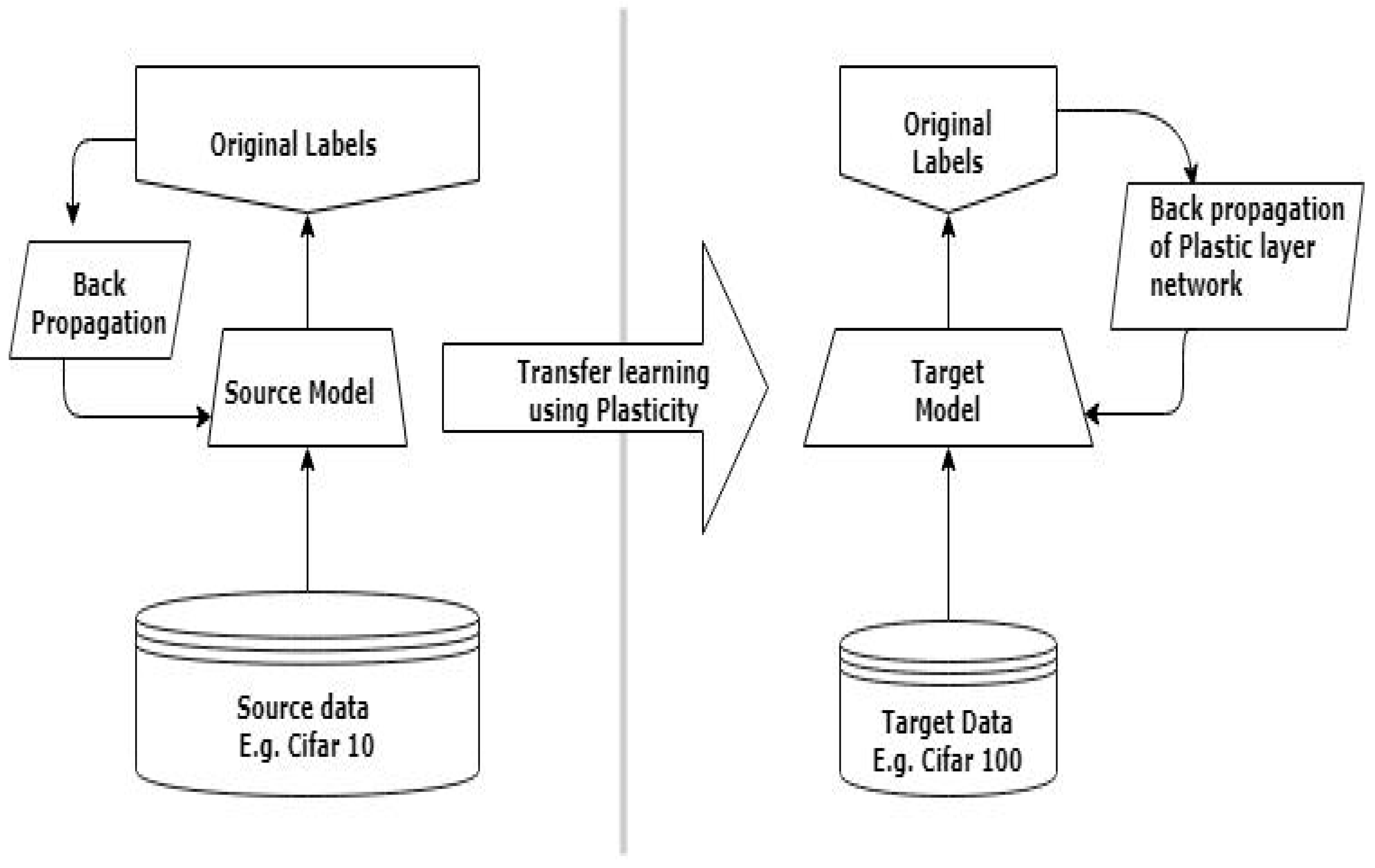
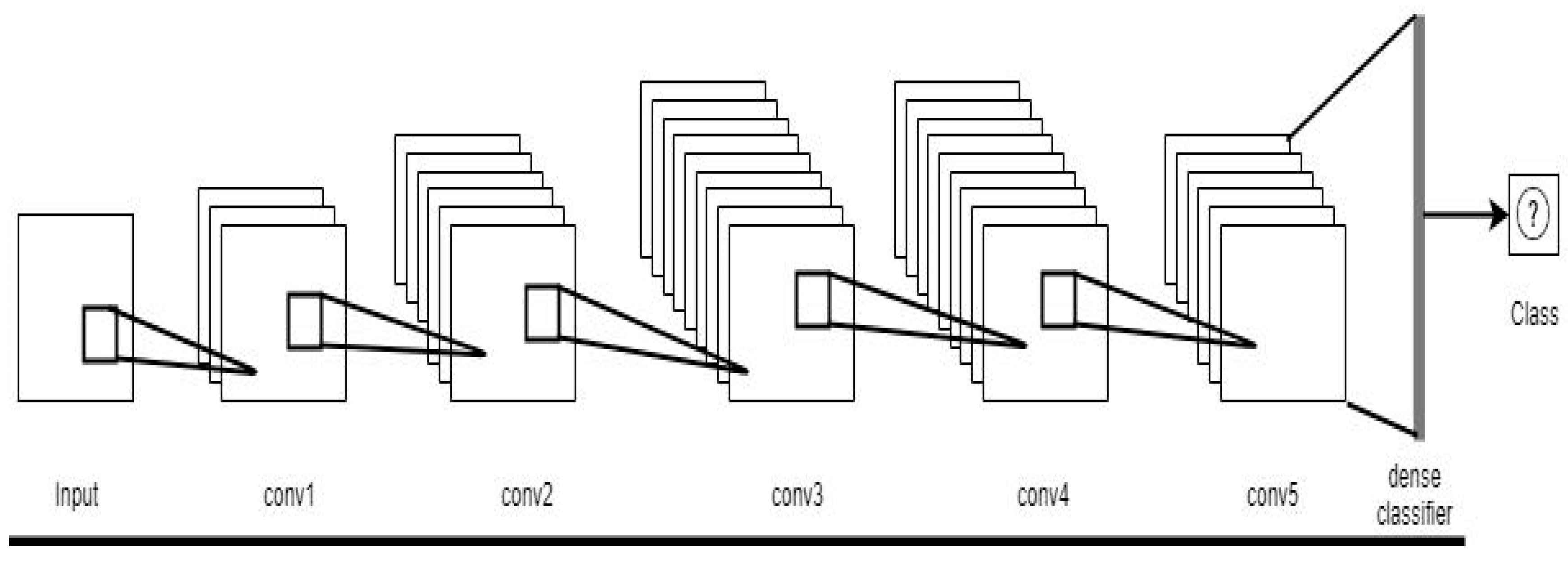
In this paper, we present an algorithm called Hebbian Transfer Learning (HTL), which performs transfer learning on convolutional neural networks with synaptic plasticity in connection weights. It modifies the connection weights and also controls the plasticity coefficients [38,39,40] that are responsible for the flexible nature of each connection weight. By using the flexible nature of the network, we have defined the network layers and connection weights of a convolution neural network in multi-part [30], a static and dynamic part. The active part can adjust depending upon the input and the plasticity coefficients. Hence, we can say that the network is performing transfer learning to adapt the connection weights as per the given task. These parameters are both learned and updated during the process of training. To check the effectiveness of the proposed algorithm, experiments are performed with publicly available CIFAR-10 (Canadian Institute for Advanced Research) and CIFAR-100 image datasets. The experimental results show that the proposed transfer learning algorithm with Hebbian learning principle outperforms standard transfer learning approach, especially when the source and target domain are heterogeneous.

Main contributions and highlights of the proposed method: the key contribution of this work is to provide a CNN-based hybrid transfer-learning approach using different source pre-trained models to transfer knowledge with the hybrid approach and architecture to accomplish higher accuracy compared to the standard algorithm. The HTL algorithm is the core of the proposed technology. In the proposed method, our aim is to utilize the existing CNN algorithm and do fusion work (e.g., interface work for biology and technology as a research domain). By applying Hebbian learning in transfer learning and deep learning, this method is reusable. It can be used to accelerate the training of neural networks. It is a hybrid CNN architecture.

We propose flexible architecture and algorithms, easy to extend algorithms to other deep learning techniques and domains. First time plasticity is applied in transfer learning. We merge multiple solutions to generated optimal solution using algorithm. These applied methods are well proved biologically by Donald O. Hebb. In larger view, we have made conceptual contribution towards transfer learning in deep learning. In addition, the paper also provides the methodological details of the work, which can be utilized by any research group to take the benefit of this work. Therefore, the motivation of the present study was to utilize the power of Hebbian learning rules and machine learning, and enable better accuracy. The idea of proposed Hebbian learning is to let a new algorithm inherit the knowledge of the existing algorithm. Just as the teacher teaches the student knowledge, the higher level of summary knowledge transfer is undoubtedly the fastest and most efficient.

The rest of the paper is divided in the following section: Section 2 summarizes related works. Section 3 describes the methodology used in the study, where the details of the problem definition, proposed algorithm, and technical logics are discussed in detail. Section 4 provides the experiments, and results of the classification algorithms, describing datasets for training and testing, the comparative performance of training and testing accuracy for both HTL and standard transfer learning (STL) algorithms is studied, and the results with data-plots are discussed in this section, which is followed by a discussion section. Finally, the conclusion is presented in Section 5.

2. Related Works

2.1. Feature Extraction and Deep Learning

Materials Feature extraction is a key process in computer vision, and there has been a large amount of work in literature. Article [41] proposed a method named local binary patterns (LBP) to extract the local neighborhood information. It has proved to be efficient in many computer vision algorithm as it has simple and very computationally efficient implementation. In specific detail, a way to extract and retrieve invariant local features, ref. [42] proposed the idea of local ternary patterns (LTP). Among others, local tetra patterns [43] extract multidirectional information and obtain more robust data. Another approach, such as CBIR, uses a combination of the local feature descriptor and artificial neuron [44]. Further, ref. [45] proposed scale-invariant feature transform (SIFT) to detect the scale-invariant interest points (SIIP). Speed up the robust feature extraction (SURF) introduced by [46] reduces the computational complexity of SIFT. The researchers integrate the interest points detected by SIFT/SURF with another feature descriptor and proposed a different robust feature descriptor for image classification and computer vision tasks [47].

Deep learning is one of the most popular of machine learning algorithm for computer vision [48,49]. Computer vision research witnessed drastic enhancements in image classification algorithms by moving from handcrafted features to automated learning algorithms to improve accuracy. In current computer vision technologies, this automatic way of feature extraction is the most accurate learning models for object detection and classification. Various deep learning models have been successfully applied to unsupervised, semi-supervised, and supervised learning. Applications, such as semantic segmentation, image super-resolution, object recognition, image classification benefit from the robust feature extraction and learning mechanism of Convolutional Neural Network (CNN). The performance of the system depends on the large number of training data and computing power. In [50], the author provided a survey of deep learning and its network architectures. The paper concludes that training data size and the number of training epoch affect the accuracy of the training model. However, with transfer learning, need of data and exhaustive training can be reduced.

2.2. Transfer Learning

Deep learning algorithms have achieved excellent performance with large amounts of labeled data [19]. Without sufficient amount of data for training, one cannot expect good performance in deep learning. People have been using procedures like data augmentation to increase the amount of available data that can be used for training deep learning models. However, we know that humans can learn from a small amount of data, using good analogy, experience, and knowledge acquired in the corresponding domain.

Transfer learning is a way of transferring knowledge learned from one task to another task [51,52,53,54]. A machine learning model trained on a source dataset can boost the performance of the model training on a different homogeneous or heterogeneous target dataset. For example, a deep learning model can be developed and trained for one image classification task, and then used on a second related image classification task to maximize the classification accuracy after fine-tuned with target task’s training data. To bridge the various gaps for the transfer of knowledge for CNN models, an efficient transfer method is adapting a pre-trained model for a new task, called fine-tuning [55]. In the standard transfer learning example, a model is trained with a large volume of data, and learns model parameter weights and bias. Then, the model is embedded to a new model for target task that can be initialized with pre-trained weights and fine-tuned with target dataset [56].

The target applications for Hebbian transfer learning can be anything, such as image segmentation, object recognition for robotic manipulation, pedestrian or obstacle detection for autonomous vehicles, among others.

2.3. Hebbian Principle

In [57], Hebb presented various biologically inspired research and investigated human brains mechanism of learning a higher complex concept based on an initial education of basic idea. In further work, an algorithm based on initial research on how human vision utilizes the principle—neurons that fire together wire together, neurons that fire out of sync fail to link—is proposed. The algorithm applies the behavioral learning principles and mathematical practices on how adjacent neurons firing together strengthens the corresponding connection in an animal brain. The work of [58], about half a century ago, explained a lot about the development and plasticity of the real brain cells. They investigated the neural response behavior, in general, called plasticity. They worked on construction, organization, and plasticity of the brain, patterned activity, and many other functions of plasticity. Their study on the visual cortical circuit and its relationship to particular learning to induce plasticity have proved to be of great significance [59].

Agent’s ability that can learn from experience can be treated as meta-learning or the problem of learning of the learning [60,61,62]. Hebbian learning is a very discriminative type of meta-learning study. In [63], the similar approach of using additional “fast weights” along with the standard neural network structure is proposed. The function of fast weights is to decrease or increase the connection weights in the wake of neural activity. To be specific, it strengthens the neural connections in the effect of the recently learned pattern [64]. The significance of using synaptic plasticity in neural networks as a source of transfer learning has enormous potential. Plasticity at the very local level of a neuron-to-neuron connection, when used as an enhancement to neural network, may learn any independent memory behavior. However, in a human brain cell or animal brain, the plasticity percentage varies differently in every connection between neurons. Those connections can have similar values and can save memories over years that may not be possible with “fast weights.”

The discrimination caused by pre and post spike activation of electric signals in brain neurons makes it a very viable candidate for study of transfer learning in neural networks. The algorithm proposed in this paper, named Hebbian transfer learning, employs the behavioral knowledge of Hebbian learning rules stated by Donald O. Hebb in his work.

2.4. Motivation and Significance of Proposed Methodology

Our aim is to utilize the existing CNN algorithm and do fusion work, where we merge multiple solutions to generate optimal solution or algorithm (like the best of both techniques). Creating interface or intermediate work for biology and technology as a research field. Hebbian learning is already a well-established field with well-proven rules (since the last 50 years). Integrating it with a modern algorithm is a good approach in problem solving. We applied Hebbian learning to knowledge transfer in deep learning neural nets. It is a method for reusing a model trained on a related predictive dataset.

It can be used to accelerate the training of neural networks as either a weight initialization scheme or feature extraction method.

2.5. Need for Such Fusion Work

Artificial neural networks were previously limited in its ability to solve actual problems, due to the vanishing gradient and overfitting problems with training of deep architecture, lack of computing power, and primarily the absence of sufficient data to train the computer system. A solution for few of these problems is availability of big data, and enhanced computing power with the current graphics processing units. However, another alternative to the problem of need for large data and computing power is transfer learning in neural networks. A lot of time and experience are required to annotate medical images and images in general as well, and that is where transfer learning can play a significant role: it allows for the use of a pre-trained architecture that was, the most appropriate TL technique in a situation with deficient datasets. The proposed technique can help in overcoming the scarcity of images. Importance of choosing an appropriate method can make these problems go away and transfer learning with the Hebbian learning algorithm is a good solution to the above-talked problems in neural network training algorithms, such as CNNs.

3. Hebbian Transfer Learning

3.1. Problem Definition

This section presents the problem definitions and notations used for description of our algorithm, following those of [56].

A task $\mathcal{T}$ is defined by a label space $\mathcal{Y}$ and a predictive function $f(·)$. The predictive function is learned from a dataset $\mathrm{D}=\left\{x_i,y_i\right\}$ to predict the label value of a data. A domain $\mathcal{D}$ is defined by a feature space $\mathcal{X}$ and provided by a dataset $\mathrm{D}=\left\{x_i,y_i\right\}$ where $x_i\in \mathcal{X}$ and $y_i\in \mathcal{Y}$.

Given a source domain ${\mathcal{D}}_S$ with a corresponding task ${\mathcal{T}}_S$ and a target domain ${\mathcal{D}}_T$ with a corresponding task ${\mathcal{T}}_T$, transfer learning is the process of improving the learning of the target predictive function $f_T$(∙) by using dataset in ${\mathcal{D}}_T$ and the knowledge learned from ${\mathcal{D}}_S$ and ${\mathcal{T}}_S$.

The notations we used to describe our algorithm are summarized in

Table 1. Notations used in describing the Hebbian transfer learning algorithm.

${\mathcal{T}}_S$$,{\mathcal{T}}_T$	The source task and target task
${\mathrm{D}}_{\mathrm{S}}$$,{\mathrm{D}}_{\mathrm{T}}$	The source domain dataset and target domain dataset
$W^S$$,W^T$	The source model parameters and target model parameters
$x_i\left(t\right)$	The output of neuron i at time t
$w_{i,j}$	The weight parameter of connection between neuron i and j
${\mathsf{\alpha }}_{i,j}$	The plasticity parameter of connection between neuron i and j
$Heb{b}_{i,j}\left(t\right)$	The Hebbian trace—plasticity of connection between neuron i and j
$\eta$	The learning rate of plasticity
$\sigma$	The nonlinear activation function

.

Goal: 

Our goal is to find the predictive function $f_T(·)$ for target image classification task ${\mathcal{T}}_T$ by transferring knowledge from source image classification task ${\mathcal{T}}_S$. The source and target tasks are different, i.e., ${\mathcal{T}}_S\ne {\mathcal{T}}_S$, since they have different label space, ${\mathcal{Y}}_S\ne {\mathcal{Y}}_T$. The source and target domains are also different, i.e., ${\mathcal{D}}_S\ne {\mathcal{D}}_T$, and there are source domain dataset ${\mathrm{D}}_{\mathrm{S}}$ = {($x_{S_1}, y_{S_1}$), …, ($x_{S_n}$, $y_{S_n}$)} and target domain dataset ${\mathrm{D}}_{\mathrm{T}}$ = {($x_{T_1}$, $y_{T_1}$), …, ($x_{T_n}$, $y_{T_n}$)}. The predictive function $f_T(·)$, which predicts the label $y_T$ of an image data $x_T$, is represented by neural network model parameters $W^T$.

Input: 

The target domain dataset ${\mathrm{D}}_{\mathrm{T}}$, and the neural network model parameters $W^S$ obtained from training on source task ${\mathcal{T}}_S$ and dataset ${\mathrm{D}}_{\mathrm{S}}$.

Output: 

The neural network model parameters $W^T$ for target task ${\mathcal{T}}_T$, which is obtained by fine-tuning $W^S$ using the target domain dataset ${\mathrm{D}}_{\mathrm{T}}$ with Hebbian transfer learning.

In our definition, the heterogeneous property between the source and target task has two different meanings—(1) they have different feature spaces, i.e., different image sizes and styles, or (2) they have semantically different contents, i.e., different kinds of objects in images. In the following sections, we refer to the second meaning for heterogeneity. For the experiment with CIFAR-10 as a source and a subset of CIFAR-100 as a target, they are all heterogeneous but in different degrees. For the experiment with various classes in CIFAR-100 as sources and targets, homogeneous datasets mean that the objects in images in the datasets are similar as ‘vehicle 1’ and ‘vehicle 2’, and the heterogeneous datasets mean that the objects in images in the datasets are different as ‘vehicle 1’ and ‘people’.

3.2. The Algorithm

In the conceptual process presented in Figure 1, on one side, the source parameters are learned and then on the other side, the target parameters are fine-tuned from the transferred parameters. The source model is trained using standard backpropagation, while the target model is trained using the backpropagation of plastic layer for Hebbian learning [65]. In the experiment results section, we compare the result of Hebbian transfer learning with standard transfer learning, where the parameters are fine-tuned by standard backpropagation only.

For transfer learning we use the same standard CNN architecture for image classification for source and target model, explained later in detail. To describe in easy words, in the initial step, we train the source model with a source domain dataset using stochastic gradient descent. In the next step, the model parameters (connection weights) learned on the source domain dataset is used to initialize the target model to perform transfer learning. In the last step, the target model parameters are fine-tuned by using the target domain dataset (using the Hebbian transfer learning technique). Figure 1 shows the conceptual process of the plastic way of Hebbian transfer learning task.

The transfer learning setup aided by Hebbian learning principle helps to better perform feature adaptation from heterogeneous source to target domain model. The strength of each connection is governed by Hebbian plasticity during networks lifetime. The plastic neural network is a combination of a parameter, which determines baseline weights and the degree of plasticity of each connection. These parameters govern the way in which each connection changes over time as a result of experience. The Hebbian plasticity for each connection can be modeled as a time-dependent quantity called Hebbian trace $Heb{b}_{i,j}$ [64]. Equation (1) represents the simplest form of Hebbian trace, which is a running average of the product of pre and postsynaptic activities. With the Hebbian trace, the strength of a connection at time t is determined by baseline weights $w_{i,j}$ and plasticity parameter ${\mathsf{\alpha }}_{i,j}$ multiplied by $Heb{b}_{i,j}$, and it defines the response of a given output neuron as in Equation (2).

$$Heb{b}_{i,j}\left(t+1\right)=\eta x_i\left(t-1\right)x_j\left(t\right)+\left(1-\eta \right)Heb{b}_{i,j}\left(t\right)$$

(1)

$$x_j\left(t\right)=\sigma \left\{ {\displaystyle \sum }\left[w_{i,j}{x}_i\left( t-1\right)+{\alpha }_{i,j}Heb{b}_{i,j}\left(t\right)x_i\left(t-1\right)\right] \right\}$$

(2)

There are many possible formulations of Hebbian plasticity rule. In the Equation (1), the weight decay term causes Hebbian traces decay thus causing memories decay, in the absence of input. We can turn to other Hebbian rules that perform better weight value stabilization and can prevent runaway divergence, like Oja’s rule [66]. The computation of Hebbian trace implementing Oja’s rule is given in Equation (3).

$$Heb{b}_{i,j}\left(t+1\right)=Heb{b}_{i,j}\left(t\right)+\eta x_j\left(t\right)\left(x_i\left(t-1\right)-x_j\left(t\right)Heb{b}_{i,j}\left(t\right)\right)$$

(3)

In Hebbian transfer learning, an episode is one-step of training using one batch of dataset. The lifetime of the training is the training of network using the entire dataset once. The Hebbian trace $Heb{b}_{i,j}$ is dynamic during an episode, and the baseline weights and the degree of plasticity are adjusted for each episode. We conducted the experiment with CNN architecture from [67], with the execution of stochastic gradient descent (SGD). The convolution neural network model has 64, 192, 384, 384, 256 filters in the five convolutional layers, followed by a dense classifier for both source domain training and transfer learning. The proposed Hebbian transfer learning algorithm can be described as follows:

Algorithm: Hebbian Transfer Learning.

Input: ${\mathrm{D}}_{\mathrm{T}},{\mathrm{W}}^{\mathrm{S}}$              //target image datasets and source weights

Output: ${\mathrm{W}}^{\mathrm{T}}$               //target weights

1: Initialize Hebbian trace ${\mathrm{Hebb}}_{\mathrm{i},\mathrm{j}}$         //Hebbian plasticity

2: ${\mathrm{W}}^{\mathrm{T}}\leftarrow {\mathrm{W}}^{\mathrm{S}}$                 //assigning source weights to target

3: ${\mathrm{W}}^{\mathrm{T}}\leftarrow {\mathrm{W}}^{\mathrm{T}}-{\mathrm{W}}_{\mathrm{i},\mathrm{n}}^{\mathrm{T}}$             //removing last layer weights of CNN

4:   for episode in range(episodes) do:

for batch_idx, (inputs, targets) in enumerate(trainloader):

5:      ${\mathrm{x}}_{\mathrm{j}}\left(\mathrm{t}\right)=\mathsf{\sigma }\left\{{\mathsf{\Sigma }}_{\mathrm{i}=\mathrm{inputs}}\left[{\mathrm{w}}_{\mathrm{i},\mathrm{j}}{\mathrm{x}}_{\mathrm{i}}\left(\mathrm{t}-1\right)+{\mathsf{\alpha }}_{\mathrm{i},\mathrm{j}}{\mathrm{Hebb}}_{\mathrm{i},\mathrm{j}}\left(\mathrm{t}\right){\mathrm{x}}_{\mathrm{i}}\left(\mathrm{t}-1\right)\right]\right\}$

6:      ${\mathrm{Hebb}}_{\mathrm{i},\mathrm{j}}\left(\mathrm{t}+1\right)={\mathrm{Hebb}}_{\mathrm{i},\mathrm{j}}\left(\mathrm{t}\right)+{\mathsf{\eta }\mathrm{x}}_{\mathrm{j}}\left(\mathrm{t}\right)\left({\mathrm{x}}_{\mathrm{i}}\left(\mathrm{t}-1\right)-{\mathrm{x}}_{\mathrm{j}}\left(\mathrm{t}\right){\mathrm{Hebb}}_{\mathrm{i},\mathrm{j}}\left(\mathrm{t}\right)\right)$

7:    if episode % k == 0:                  //k is an adjustable parameter

8:      Calculate B.C.E loss and Backpropagate      //gradient descent

9:      hebb = model.module.initialZeroHebb()

10:     ${\mathrm{W}}^{\mathrm{T}}\leftarrow {\mathrm{W}}^{\mathrm{T}}-\Delta {\mathrm{W}}_{\mathrm{i},\mathrm{j}}^{\mathrm{T}}$

11:   return ${\mathrm{W}}^{\mathrm{T}}$

3.3. CNN Hybrid Architecture

We implemented our experiment with CNN architecture from the [67]; we used only single graphics processing unit (GPU) training, with the execution of SGD. In detail, the convolution neural network model has 64, 192, 384, 384, 256 filters in the five convolutional layers, respectively. It is followed by a dense classifier for standard learning and standard transfer learning. In the scenario of the synaptic plastic network, the plastic layer replaces the network’s classifier layer, when the network is learning and model is fine-tuning. It back-propagates the error that plastic network is utilizing in the transfer-learning scenario. This CNN architecture is used in the CIFAR-10 and CIFAR-100 transfer learning experiment. The architecture has five convolutional layers, with max pooling after every convolutional layer, and rectified linear unit (Relu) as the non-linear unit. There is a dense plastic layer following the five convolutional layers, which has $Heb{b}_{i,j}$ the Hebbian trace that defines the plasticity of the every connection weight in the last network layer, which results in the required number of class output.

3.4. Significance of Hybrid Architecture

We chose this architecture because it has been studied in detail by many other research groups [67]. Moreover, to introduce a new idea, it is more important to use a commonly studied architecture where it’s more understandable to conceive the proposed ideas by a relatively new reader on the domain. The proposed architecture is a hybrid and combination of standard CNN layers and additional plastic neural network layers. Such architecture has never been used before for transfer learning techniques. This approach makes use of Hebbian plasticity for exploiting the existing weight parameters with additional plastic values (Please refer Figure 2). It is an optimal solution because, with minimum change in existing techniques, we can achieve the targeted desired objective. For example, with the introduction of a newly born infant, the whole design of a car and it usefulness is unaccommodating. As the existing seat of a car is too large for a baby. Thus, we do not replace the entire seat to accommodate a small baby. We add a baby seat in the existing car design.

Similarly, the existing methods enhanced with plasticity will accommodate small changes to the parameters of the CNN layers. That makes weight adaptation a quick (and faster) process. This discriminating property of Hebbian learning employed with our proposed algorithm makes it a significant approach to techniques such as transfer learning, where relative minor weight fine tuning, using the pre- and post-spikes of a neural network, such as structure, enhance the targeted unfamiliar dataset domain adaptation possible.

4. Experiments

4.1. Experimental Setup

We perform two sets of experiments. In experiment A, we use the benchmark dataset CIFAR-10 as source domain and CIFAR-100 as target domain. In experiment B, we use part of CIFAR-100 as both source and target domain. The CIFAR-10 dataset consists of 32 × 32 color images in 10 classes, with 6000 images per class. The CIFAR-100 dataset consists of 32 × 32 color images in 100 classes, with 600 images per class. In CIFAR-100, the 100 classes are grouped into 20 super classes. We have already explained the hybrid CNN-plastic architecture in Figure 2. The figure is the exact architecture using exact number of CNN and plastic layers as described in Section 3.3. Conceptualization and data recording was performed by experimentation with datasets CIFAR-10 and CIFAR-100.

During the study the algorithm “Hebbian Transfer Learning”, was created and then coded in python using PyCharm (Version: 2018.2) complier and python version 2.7 and 3.0 using PyTorch libraries, along with other dependencies. All of the recorded data were studied in depth by all of the manuscript authors. Over the period of multiple months, we studied the data and plotted the data graphs (Figure 3 and Figure 4).

4.1.1. Dataset for Experiment A

This section presents the description of the source and target task datasets for experiment A.

The CIFAR-10 dataset consists of 50,000 training images and 10,000 test images. The classes are completely mutually exclusive. There is no overlap between automobiles and trucks. For example, “Automobile” includes sedans, SUVs, things of that sort. “Truck” includes only big trucks.

Table 2. The source dataset classes from CIFAR-10.

Dataset	Classes
S	airplane, automobile, bird, cat, deer, dog, frog, horse, ship, truck

display the collection of all the ten classes in the dataset CIFAR-10, in alphabetical order.

The CIFAR-100 dataset is just like the CIFAR-10, except there are 500 training images and 100 testing images per class. Each image comes with a “fine” label (the class to which it belongs) and a “coarse” label (the superclass to which it belongs). The binary version of the CIFAR-100 is just like the binary version of the CIFAR-10, except that each image has two label bytes (coarse and fine) and 3072 pixel bytes.

Table 3. The 10 target datasets created from CIFAR-100.

Dataset	Classes (Union of Similar 2 Super Classes)
${\mathrm{T}}_1$	aquatic mammals + fish: beaver, dolphin, otter, seal, whale, aquarium fish, flatfish, ray, shark, trout
${\mathrm{T}}_2$	flowers + fruit and vegetables: orchids, poppies, roses, sunflowers, tulips, apples, mushrooms, oranges, pears, sweet peppers
${\mathrm{T}}_3$	food containers + household electrical devices: bottles, bowls, cans, cups, plates, clock, computer keyboard, lamp, telephone, television
${\mathrm{T}}_4$	household furniture + large man-made outdoor things: bed, chair, couch, table, wardrobe, bridge, castle, house, road, skyscraper
${\mathrm{T}}_5$	insects + non-insect invertebrates: bee, beetle, butterfly, caterpillar, cockroach, crab, lobster, snail, spider, worm
${\mathrm{T}}_6$	medium-sized mammals + small mammals: bear, leopard, lion, tiger, wolf, camel, cattle, chimpanzee, elephant, kangaroo
${\mathrm{T}}_7$	medium-sized mammals + small mammals: fox, porcupine, possum, raccoon, skunk, hamster, mouse, rabbit, shrew, squirrel
${\mathrm{T}}_8$	people + reptiles: baby, boy, girl, man, woman, crocodile, dinosaur, lizard, snake, turtle
${\mathrm{T}}_9$	trees + large natural outdoor scenes: maple, oak, palm, pine, willow, cloud, forest, mountain, plain, sea
${\mathrm{T}}_{10}$	vehicles 1 + vehicles 2: bicycle, bus, motorcycle, pickup truck, train, lawn-mower, rocket, streetcar, tank, tractor

, display all the classes from CIFAR-100 used as target task dataset in experiment A. The dataset is divided into 10 major groups depending on the similarity of the coarse label. For example dataset ${\mathrm{T}}_1$, combines data from two super classes “aquatic mammals” and ”fish”. The aim is to create multiple target datasets for experimentation and result comparison.

4.1.2. Dataset for Experiment B

This section presents the description of the source and target task datasets for experiment B.

The source and target datasets are subsets from CIFAR-100. The entire experimentation data is segregated into eight different groups.

Table 4. Datasets from CIFAR-100 used for source and target in experiment B.

Dataset	Classes
${\mathrm{D}}_1$	vehicles 1:	bicycle, bus, motorcycle, pickup truck, train
${\mathrm{D}}_2$	vehicles 2:	lawn-mower, rocket, streetcar, tank, tractor
${\mathrm{D}}_3$	large carnivores:	bear, leopard, lion, tiger, wolf
${\mathrm{D}}_4$	large omnivores and herbivores:	camel, cattle, chimpanzee, elephant, kangaroo
${\mathrm{D}}_5$	household furniture:	bed, chair, couch, table, wardrobe
${\mathrm{D}}_6$	household electrical devices:	clock, computer keyboard, lamp, telephone, television
${\mathrm{D}}_7$	people:	baby, boy, girl, man, woman
${\mathrm{D}}_8$	reptiles:	crocodile, dinosaur, lizard, snake, turtle

display all the eight datasets, along with fine label and coarse label. Each super class has five subclasses as described in the Table 4.

The aim is to group and perform experiment among homogeneous and heterogeneous datasets.

4.2. Experiment Study

4.2.1. Experiment A: CIFAR-10 to CIFAR-100 Transfer

In the first experiment, we use all 10 classes of the CIFAR-10 for source domain training to get the parameters $W^S$. For the target domain, we made 10 different subsets of CIFAR-100 categories by grouping 2 similar superclass categories together like ‘aquatic mammals’ and ‘fish’, and performed fine-tuning for those 10 subsets and compared the accuracy. Table 2 and Table 3 describe the source and target datasets for experiment A.

First, we trained the CNN model on the CIFAR-10 dataset for the classification task on ten different data classes. Under our experimental setup, we set the learning rate of {0.0001, 0.00001, 0.000001}, which, after reaching a particular epoch level, decreases by unit place. Training batch size used as one image per training cycle. We use cross-entropy loss.

Second, we use the pre-trained model in the heterogeneous source domain to initialize the model for transfer learning on the target domain. The last layer of CNN is set to random values. Our experimental setup for fine-tuning the connection weights for transfer learning. We used a standard fine-tuning algorithm to do transfer learning on ten different category classes subsets, from CIFAR-100 datasets (as described in Table 3). Cross-entropy loss is used as in training source dataset.

Next, we repeat the experiment with the same pre-trained model using our proposed transfer learning algorithm, Hebbian transfer learning. The experimental setup for fine-tuning the connection weights for transfer learning is same as source domain training. It works in phases, where a lifetime is mapped to one epoch or one cycle of the fine-tuning process [64].

Each lifetime contains n-number of episodes; n is a meta-parameter for the algorithm. At each time step, a transfer learning process uses a batch size of 1, which is for one iteration of a forward pass for the CNN and the Hebbian trace is updated. At the end of each episode, we calculate loss and compute the eta (n) and alpha (α) by using backpropagation and update $w_{i,j}$ and ${\alpha }_{i,j}$ by using backpropagation. After every episode, Hebbian trace is re-initialized to all zero.

$$BCE=-\frac{1}{N}{\displaystyle \sum }_{i=0}^N{y}_i.log\left(y_i^{^}\right)+\left(1-y_i \right).log\left(1-y_i^{^}\right)$$

(4)

HTL propagate back the gradient at the end of each episode as mentioned above. For keeping the configuration comparable, the validation loss function is used in HTL transfer learning setup, cross-entropy. To calculate the gradient, the loss is calculated using Equation (4). The error is then back propagated. For keeping the configuration comparable, i.e., the validation loss function used in HTL is kept the same as the one used in standard transfer learning setup, Cross-entropy. We record validation loss, top-1, and top-5 accuracy results for each lifetime. We must note here that, for each epoch in the standard transfer learning algorithm, SGD is performed, which is for each training image, because the batch size is 1. However, in Hebbian transfer learning, the algorithm only back- propagates at the end of each episode, after every n-time steps. HTL is performing n-times fewer gradient updates.

4.2.2. Experiment B: CIFAR-100 to CIFAR-100 Transfer

In the second experiment, we selected eight super classes from CIFAR-100 into four groups of semantically similar categories, to compare the efficiency of proposed algorithm for transfer learning with homogeneous and heterogeneous sources. Table 4 shows the datasets selected for experiment B. Among the datasets, ${\mathrm{D}}_1$-${\mathrm{D}}_2$, ${\mathrm{D}}_3$-${\mathrm{D}}_4$, and ${\mathrm{D}}_5$-${\mathrm{D}}_6$ are homogeneous (semantically similar) datasets, while ${\mathrm{D}}_7$ and ${\mathrm{D}}_8$ are heterogenous to those datasets. The experimental setup is same as the experiment A.

4.3. Experimental Results

4.3.1. Experimental Results: Experiment A

Table 5. Top-1 and Top-5 validation accuracies of standard transfer learning (STL) and HTL for experiment A.

Metric	Source	Target	STL	HTL	Improvement
Top-1 accuracy	S	${\mathrm{T}}_1$	59.6%	60.1%	+0.50%
		${\mathrm{T}}_2$	69.9%	71.7%	+1.80%
		${\mathrm{T}}_3$	65.0%	65.5%	+0.50%
		${\mathrm{T}}_4$	75.0%	75.8%	+0.80%
		${\mathrm{T}}_5$	67.9%	70.2%	+2.30%
		${\mathrm{T}}_6$	63.0%	63.8%	+0.80%
		${\mathrm{T}}_7$	57.0%	57.3%	+0.30%
		${\mathrm{T}}_8$	51.6%	54.2%	+2.60%
		${\mathrm{T}}_9$	73.7%	74.5%	+0.80%
		${\mathrm{T}}_{10}$	74.4%	75.9%	+1.50%
Average			65.71%	66.90%	+1.19%
Top-5 accuracy	S	${\mathrm{T}}_1$	94.7%	95.1%	+0.40%
		${\mathrm{T}}_2$	97.3%	97.9%	+0.60%
		${\mathrm{T}}_3$	94.9%	96.0%	+1.10%
		${\mathrm{T}}_4$	97.8%	98.0%	+0.20%
		${\mathrm{T}}_5$	95.0%	95.3%	+0.30%
		${\mathrm{T}}_6$	94.0%	94.4%	+0.40%
		${\mathrm{T}}_7$	91.0%	91.1%	+0.10%
		${\mathrm{T}}_8$	95.5%	96.4%	+0.90%
		${\mathrm{T}}_9$	99.0%	99.4%	+0.40%
		${\mathrm{T}}_{10}$	97.9%	98.3%	+0.40%
Average			95.71	96.19	+0.48%

shows the comparison of standard transfer learning (STL) and Hebbian transfer learning (HTL) in terms of top-1 and top-5 validation accuracies for experiment A, as described in Section 4.2.1.

The results show that in all cases, the HTL outperforms STL. In particular, top-1 accuracy for target dataset ${\mathrm{T}}_8$ shows lowest accuracy but highest improvement of +2.60% with HTL, which implies that the HTL is more effective for transfer learning between heterogeneous source and target.

In average, the improvement of top-1 accuracy with HTL is +1.19%, and the improvement of top-5 accuracy with HTL is +0.48%.

4.3.2. Experimental Results: Experiment B

Table 6. Top-1 validation accuracies of STL and HTL for experiment B.

Metric	Source	Target	STL	HTL	Improvement
Top-1 Accuracy	${\mathrm{D}}_1$	${\mathrm{D}}_2$ (Homogeneous)	73.2%	73.2%	0.0%
	${\mathrm{D}}_1$	${\mathrm{D}}_7$ (Heterogeneous)	37.8%	40.2%	+2.4%
	${\mathrm{D}}_3$	${\mathrm{D}}_4$ (Homogeneous)	67.4%	67.2%	−0.2%
	${\mathrm{D}}_3$	${\mathrm{D}}_7$ (Heterogeneous)	42.2%	43.6%	+1.4%
	${\mathrm{D}}_5$	${\mathrm{D}}_6$ (Homogeneous)	72.2%	72.8%	+0.6%
	${\mathrm{D}}_5$	${\mathrm{D}}_8$ (Heterogeneous)	62.4%	63.8%	+1.4%
Average accuracy for Homogeneous case			70.93%	71.06%	+0.13%
Average accuracy for Heterogeneous case			47.46%	49.20%	+1.80%

shows the comparison of STL and HTL in terms of top-1 validation accuracies for experiment B setup.

In this experiment, both the source dataset and target dataset are subsets of CIFAR-100, but we tried transfer learning with various combinations of homogenous and heterogeneous (semantically different) source/target as described in Section 4.2.2. The results show that STL and HTL get almost similar accuracies for homogenous source-target pairs, but HTL clearly outperforms STL for heterogeneous source-target pairs. The average accuracy improvement of HTL on heterogeneous case is +1.80%, while the average accuracy improvement of HTL on homogeneous case is only +0.13%.

The result implies that HTL is more effective for transfer learning when the source and target datasets are heterogeneous.

4.3.3. Result Data-Plots: Experiment A

The following figures, Figure 3 and Figure 4, shows the data plots for the results recorded from the experiments.

These data plots are very significant and helps to easily understand the effectiveness of plasticity influenced HTL algorithm. Here STL means standard or traditional transfer learning algorithm, and HTL is short for our purposed Hebbian transfer learning algorithm. The red color of the curve represents HTL results, and black colored curve represents the STL results, respectively. While studying the data plots in Figure 3, it is recommended to study dataset from Table 2 and Table 3. Figure 3 is also comparable to the corresponding validation accuracies from Table 5.

The results from data-plots in Figure 3 can be used for quick understanding of the results from experiment A.

Figure 3. The learning curves of STL and HTL for 10 different target dataset. Data plots (a–j) are curves with comparison results displaying data from Table 5 using datasets from Table 2 and Table 3.

Figure 3. The learning curves of STL and HTL for 10 different target dataset. Data plots (a–j) are curves with comparison results displaying data from Table 5 using datasets from Table 2 and Table 3.

The comparison of learning curves of STL and HTL for 10 different datasets in terms of top-5 accuracy are shown in Figure 3. The x-axis represents the number of epochs and the y-axis represents the validation accuracies. In each graph, the black color is for STL and the red color is for HTL. Looking at the graphs, we can observe that the Hebbian transfer learning adapts to target domain a little more slowly but eventually achieves higher validation accuracy in all cases. Again, the data curves of STL and HTL for target dataset (${\mathrm{T}}_{1-10}$), shows highest improvement in top-5 accuracy for HTL algorithm.

4.3.4. Result Data-Plots: Experiment B

Figure 4 shows the learning curves of STL and HTL for homogenous and heterogeneous cases. In Figure 4a, the source dataset is five classes dataset of superclass “vehicle 1”, and the target dataset is five classes dataset of superclass “vehicle 2”, which is homogeneous case. In Figure 4b, the source dataset is five classes dataset of superclass “vehicle 1”, and the target dataset is five classes dataset of superclass “people”, which is heterogeneous case. The results show that the proposed Hebbian transfer learning performs much better than standard transfer learning on the heterogeneous dataset scenarios.

Figure 4. The learning curves of STL and HTL for homogeneous and heterogeneous datasets. Data-plot, (a,b) show experiment results discussed in Table 6, using dataset from Table 4.

Figure 4. The learning curves of STL and HTL for homogeneous and heterogeneous datasets. Data-plot, (a,b) show experiment results discussed in Table 6, using dataset from Table 4.

4.4. Innovative Features

We present the innovations from the application point of view and innovative features of our proposal, with respect to adopted logic and proposed technique.

Introduction of biologically inspired motivations and biologically derived mathematical equations have been studied concerning transfer learning in convolution neural networks for the first time.

The hybrid architecture where the combination of a CNN traditional network and appended with plastic layer at the end is studied for the very first time for transfer learning in the object classification and object recognition domain. The existing stochastic gradient decent does fine job. However, combining the dynamics of Hebbian learning rules with existing transfer learning standard CNN algorithms make it a very significant approach. This introduction of hybrid algorithm and hybrid architecture can be applied and made use of in various applications, such as image classification, video classification, and object detection and object tracking task. As the Hebbian rules are used mathematically in this algorithm, the algorithm can be easily extended for the applications in other form of applied transfer learning in related deep learning neural network domains.

4.5. Discussion

The key element of the success of deep learning is based on the capability of the neural networks to learn high-level abstractions from input raw data through a general purpose learning procedure [68].

An important finding to emerge in this study is that even a small amount of prior knowledge from a source dataset could result in a fair measure of accuracy for predicting performance in a related target task. This indicates that there is a slight uncertainty about the transferability level of a predictive model. The definition of what is a “transferable” model is where this ambiguity lies. A model trained on a source is considered “transferable” if it achieves respectively fair results on a different dataset, related course [69]. We believe this is yet another important attempt towards transfer knowledge in the educational field.

All these advancements in deep learning make it a prominent part of the medical industry. Deep learning can be used in wide variety of areas, such as the detection of tumors and lesions in medical images [70,71]. Transfer learning in deep learning and neural networks has achieved great results in lots of domains including health domain. Several deep learning based studies have assessed the implementation of lung cancer screening CAD (Computer-Aided Diagnosis) systems [72,73,74,75,76,77,78,79,80,81,82,83,84], and show the potential for predicting lung cancer and classifying lung nodules [72,79]. Deep learning has been applied for the identification, detection, and diagnosis and risk analysis of breast cancer [85].

Applications and Comparison

Convolutional neural network for Human Epithelial-2 (HEp-2) cell image classification, fetal hypoxia detection based on transfer learning approach is a viable solution to serious medical needs [86,87]. Transfer learning for pediatric pneumonia diagnosis, lung pattern analysis, and computer-aided diagnosis of breast ultrasound images using transfer learning are some examples where introducing technology helps doctors speed up the treatment process. It also, enhances the early detection of the symptoms of the medical condition and can help a patient in critical need by making it possible to quickly evaluate the case [18,88,89]. Applying transfer learning in biomedical image analysis is a very promising domain and supports general purpose cause [89].

The ratio of patients and available specialists in medical profession is very high, especially in case of some very critically sensitive conditions, where the professionals are over-burdened. However, with studies such as froth image analysis, by use of transfer learning and convolutional neural networks, transfer learning for diabetic retinopathy fundus image classification the treatment can be easily available to larger percentage of patients in less time [90,91]. Transfer learning method for pediatric pneumonia diagnosis [18] is a very widely applied research, as kids are easy targets for diseases like pneumonia. Transfer learning for molecular cancer classification [20] and digital mammographic tumor classification [21], where the study of computer-extracted tumor features in the task of distinguishing between benign and malignant breast lesions, can be an answer to early detection of a terminal disease.

Transfer learning using X-ray baggage security imagery where, within the context of X-ray security screening, limited availability of training for particular items of interest can, thus, pose a problem. To overcome this issue, a transfer learning paradigm, such as a pre-trained CNN, primarily trained for generalized image classification tasks where sufficient training data exists, can be specifically optimized as a later secondary process that targets (specific) this application domain [22]. Similarly, transfer learning for diabetic retinopathy fundus image classification, artificial intelligence in fracture detection [91,92], and sepsis classification [93] are a few of the progressive research domains for transfer learning. Some other interesting applied works are the millet crop images study [94], online fault diagnosis [95], and decision support from financial disclosures [96].

Transfer learning is highly applicable in other domains, such as Natural language processing (NLPs) with automatic speech recognition systems [97]. Transfer learning in deep convolutional neural networks (DCNNs) is an important step in its application to medical imaging tasks. In specific cases, unsupervised transfer learning can be useful for biomedical applications [98].

Another futuristic application is using transfer learning and transferring the knowledge (connection weight parameters) from learned neural networks, such as CNNs to hardware vision devices, such as using FPGAs, so that the learned knowledge can be used in small and mobile objects, such as robots, cars, and other mobile vehicles, for example. As discussed, proposed approach can be further extended to target applications, such as image segmentation, object recognition for robotic manipulation, or pedestrian or obstacle detection for autonomous vehicles.

5. Conclusions

Transfer learning has shown significant benefits in various machine learning tasks, including image classification. The CNN architecture for image classification has feature extraction and classification layers integrated. In general, with machine learning, the training data is the same over many iterations. However, in transfer learning, the network trained with source domain data is to be fine-tuned with new target domain data, and in such situations, a biologically inspired algorithm may significantly improve the learning efficiency.

In this paper, we presented a transfer learning algorithm based on the Hebbian learning principle. The Hebbian learning represents the associative learning where simultaneous activation of brain cells positively affects the increase in synaptic connection strength between the individual cells. We investigate the use of Hebbian plasticity principles using the differentiable plasticity and backpropagation, and applied the principle to the transfer learning. In the Hebbian transfer learning method, we use the last feature extraction layer and reweight the output using a plastic layer in a way that the parameter distribution difference between the old and new training dataset is reduced. We applied HTL to CNN architecture in the experiment, but our algorithm is generic and can be extended to any neural network architecture that has feature extraction and classification layers integrated into one single entity. In this hybrid architecture, where the layers are a combination of feature extraction and plastic layer, the framework requires a minimum percentage of disturbance of weights to fine-tune the network with target dataset.

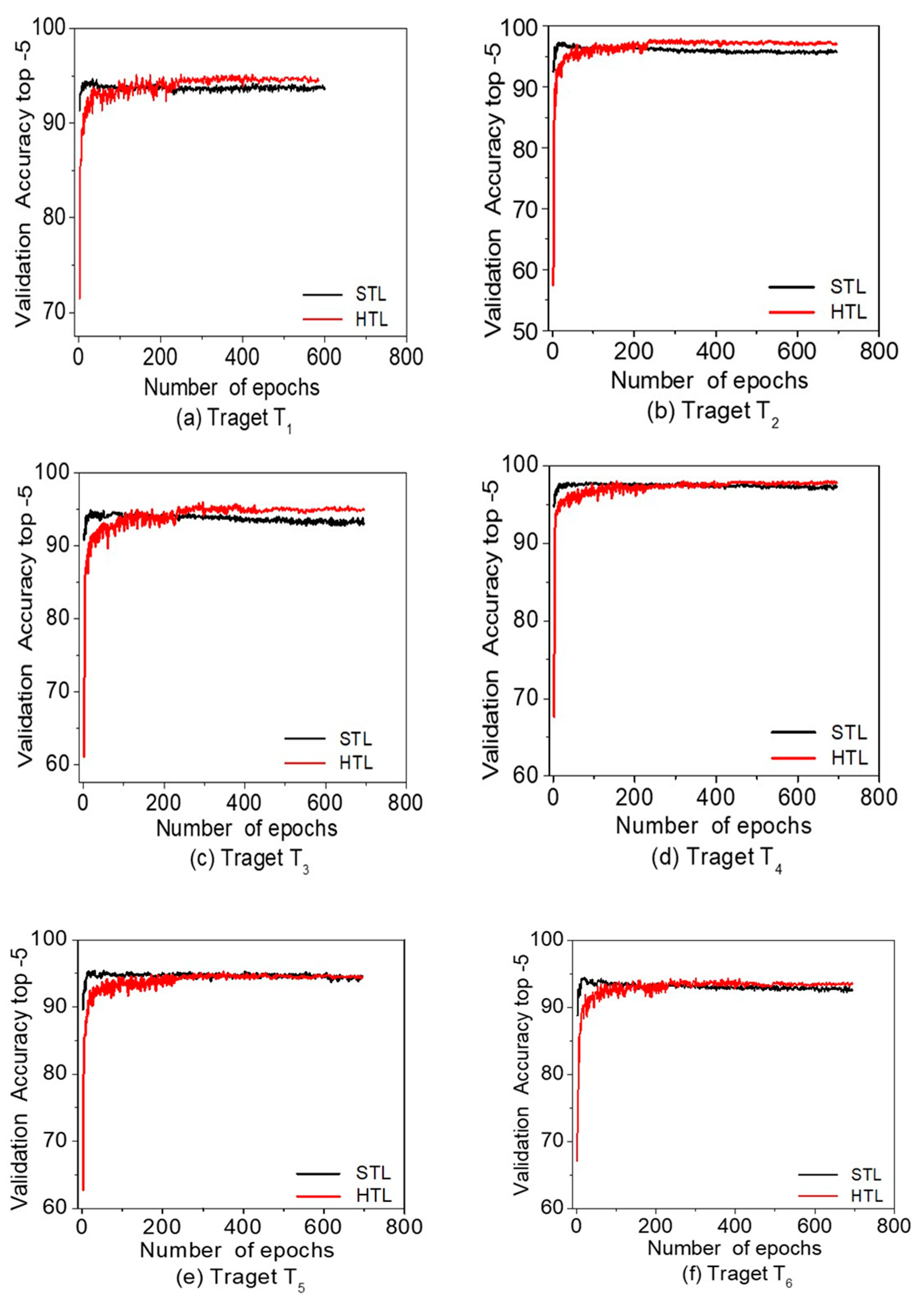
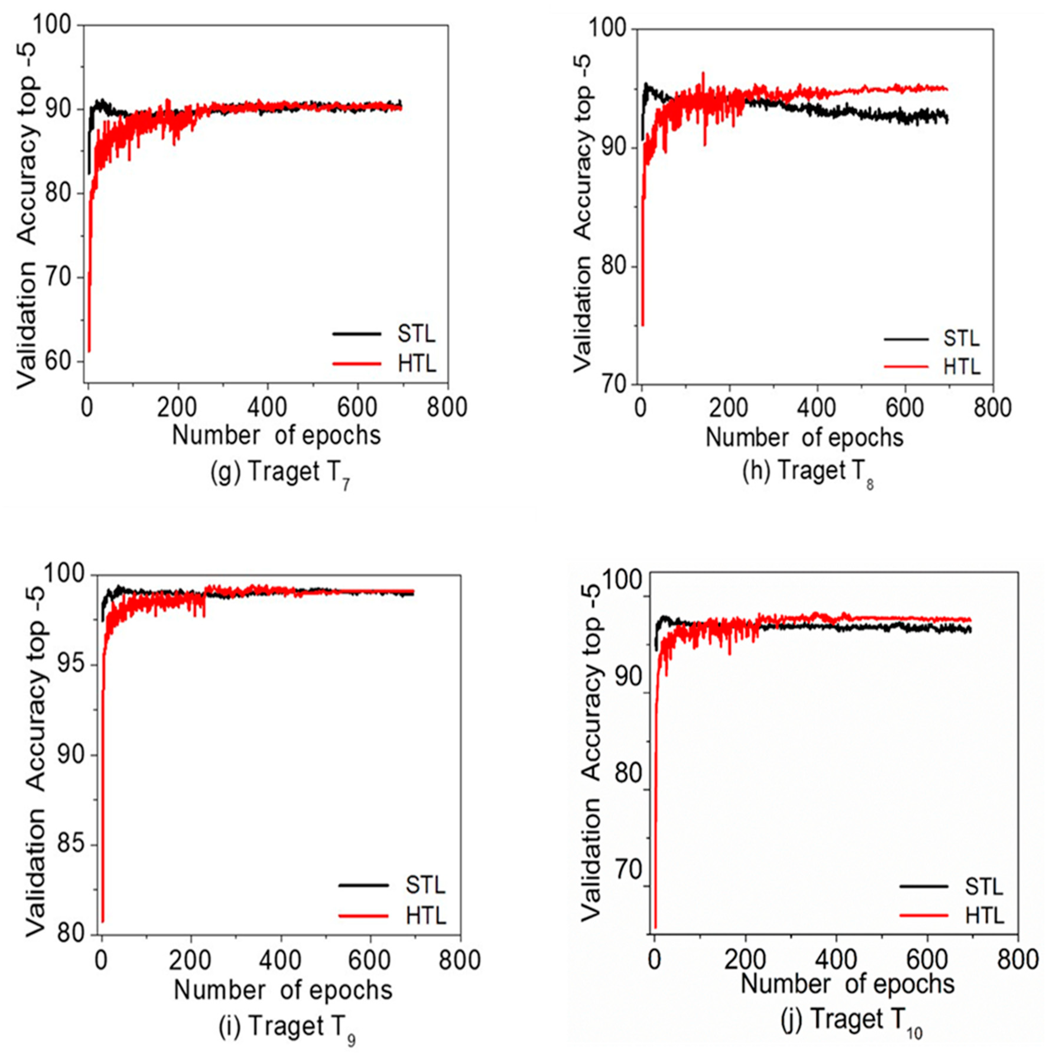
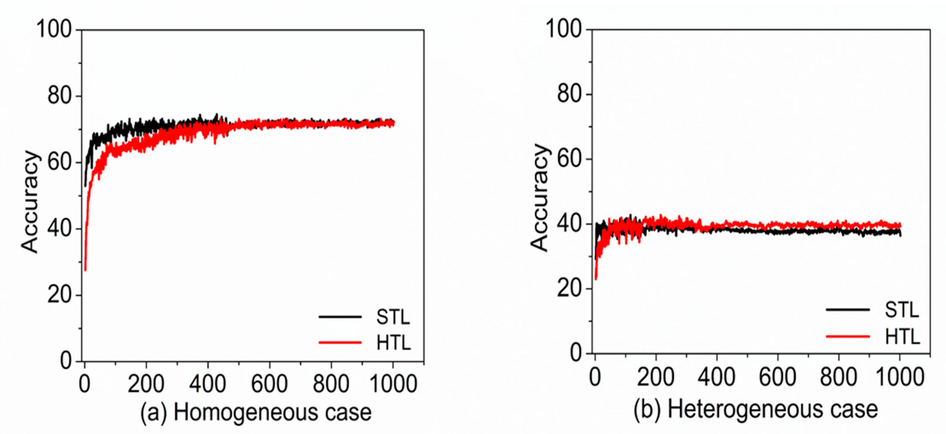
Two experiments were conducted to compare the efficiency of the proposed algorithm with standard transfer learning. The first experiment used CIFAR-10 as source domain and CIFAR-100 as target domain, and the second experiment used subsets of CIFAR-100 as both the source and target domains. The experimental results showed that in both experiments the HTL achieves better accuracy than the STL method. The average top-1 accuracy improvements are +1.19% for first experiment, and +1.80% for the second experiment. In the first experiment, it is observed that the HTL is more effective when the source and target are heterogeneous in terms of their semantic contents. In the second experiment, it is also observed that the HTL is more effective when we try transfer learning from source to heterogeneous target domain. The average top-1 accuracy improvement was +0.13% for homogeneous cases, but it was +1.80% for heterogeneous cases. On the basis of experimental results, we conclude that the proposed Hebbian transfer learning algorithm is significantly competitive to the standard transfer learning algorithm when the homogeneous source and target domain are used, and achieves much better performance when the heterogeneous source and target domain are used.

For future research, the proposed algorithm may be extended by enhancing the positive only weight change in plastic Hebbian learning part. Another possibility would be refining the CNN model by stacking additional layers and adjusting only positive weights on those layers. The algorithm may also be extended by experimenting on larger dataset, such as ImageNet for images and video datasets. Another way to extend this work is working with more advanced—and the latest—architectures, such as Inception, and other larger neural networks, DCCNs. Moreover, we may extend this algorithm to experiment with other machine learning datasets for example NLPs datasets, text datasets. In future, we may experiment with fully plastic architectures for CNNs. We may also investigate the efficiency of transfer learning in imbalanced datasets. We may utilize this quick transfer learning technique for wide range of applications in mobile objects, such as robots, cars, and other mobile vehicles using CNN parameter transfer for object detection, and many more.

References

1. Lee, J.G.; Jun, S.; Cho, Y.W.; Lee, H.; Kim, G.B.; Seo, J.B.; Kim, N. Deep learning in medical imaging: General overview. Korean J. Radiol. 2017, 18, 570–584. [Google Scholar] [CrossRef] [Green Version]
2. Rumelhart, D.E.; Hinton, G.E.; Williams, R.J. Learning representations by back-propagating errors. Nature 1986, 323, 533–536. [Google Scholar] [CrossRef]
3. Janocha, K.; Czarnecki, W.M. On Loss Functions for Deep Neural Networks in Classification. In Proceedings of the Theoretical Foundations of Machine Learning 2017, Cracow, Poland, 13–17 February 2017; Available online: https://arxiv.org/pdf/1702.05659.pdf (accessed on 21 February 2020).
4. Robbins, H.; Monro, S. A stochastic approximation method. Ann. Math. Stat. 1951, 22, 400–407. [Google Scholar] [CrossRef]
5. Krizhevsky, A.; Sutskever, I.; Hinton, G.E. Imagenet classification with deep convolutional neural networks. Adv. Neural Inform. Process. Syst. 2012, 25, 1097–1105. [Google Scholar] [CrossRef]
6. Simonyan, K.; Zisserman, A. Very deep convolutional networks for large-scale image recognition. In Proceedings of the 3rd International Conference on Learning Representations 2015, San Diego, CA, USA, 7–9 May 2015; Available online: https://arxiv.org/pdf/1409.1556.pdf (accessed on 10 April 2020).
7. Liu, N.; Wan, L.; Zhang, Y.; Zhou, T.; Huo, H.; Fang, T. Exploiting convolutional neural networks with deeply local description for remote sensing image classification. IEEE Access 2018, 6, 11215–11228. [Google Scholar] [CrossRef]
8. Alkhaleefah, M.; Wu, C.C. A hybrid CNN and RBF-based SVM approach for breast cancer classification in mammograms. In Proceedings of the IEEE International Conference on Systems, Man, and Cybernetics 2018, Miyazaki, Japan, 7–10 October 2018; Available online: https://ieeexplore.ieee.org/stamp/stamp.jsp?tp=&arnumber=8616155 (accessed on 3 March 2020).
9. Greenspan, H.; Van Ginneken, B.V.; Summers, R.M. Guest editorial deep learning in medical imaging: Overview and future promise of an exciting new technique. IEEE Trans. Med. Imaging 2016, 35, 1153–1159. [Google Scholar] [CrossRef]
10. Ching, T.; Himmelstein, D.S.; Beaulieu-Jones, B.K.; Kalinin, A.A.; Do, B.T.; Way, G.P.; Ferrero, E.; Agapow, P.M.; Zietz, M.; Hoffman, M.M.; et al. Opportunities and obstacles for deep learning in biology and medicine. J. R. Soc. Interface 2018, 15, 20170387. [Google Scholar] [CrossRef] [Green Version]
11. Wang, X.; Huang, T.-K.; Schneider, J. Active transfer learning under model shift. In Proceedings of the International Conference on Machine Learning 2014, Beijing, China, 21–26 June 2014; Available online: http://proceedings.mlr.press/v32/wangi14.pdf (accessed on 14 April 2020).
12. Tan, C.; Sun, F.; Kong, T.; Zhang, W.; Yang, C.; Liu, C. A survey on deep transfer learning. In Proceedings of the International Conference on Artificial Neural Networks 2018, Rhodes, Greece, 4–7 October 2018; Available online: https://arxiv.org/pdf/1808.01974.pdf (accessed on 6 August 2019).
13. Wang, M.; Deng, W. Deep visual domain adaptation: A survey. Neurocomputing 2018, 312, 135–153. [Google Scholar] [CrossRef] [Green Version]
14. Saito, K.; Watanabe, K.; Ushiku, Y.; Harada, T. Maximum classifier discrepancy for unsupervised domain adaptation. In Proceedings of the IEEE /CVF Conference on Computer Vision and Pattern Recognition 2018, Salt Lake City, UT, USA, 19–21 June 2018; Available online: https://arxiv.org/pdf/1712.02560.pdf (accessed on 10 March 2020).
15. Abubakar, A.; Ajuji, M.; Usman Yahya, I. Comparison of deep transfer learning techniques in human skin burns discrimination. Appl. Syst. Innov. 2020, 3, 20. [Google Scholar] [CrossRef] [Green Version]
16. Chouhan, V.; Singh, S.K.; Khamparia, A.; Gupta, D.; Tiwari, P.; Moreira, C.; Damaševičius, R.; Hugo, V.; de Albuquerque, C. A novel transfer learning based approach for pneumonia detection in chest x-ray images. Appl. Sci. 2020, 10, 559. [Google Scholar] [CrossRef] [Green Version]
17. Tsiakmaki, M.; Kostopoulos, G.; Kotsiantis, S.; Ragos, O. Transfer learning from deep neural networks for predicting student performance. Appl. Sci. 2020, 10, 2145. [Google Scholar] [CrossRef] [Green Version]
18. Liang, G.; Zheng, L. A transfer learning method with deep residual network for pediatric pneumonia diagnosis. Comput. Methods Programs Biomed. 2020, 187, 104964–104972. [Google Scholar] [CrossRef] [PubMed]
19. Raghu, M.; Zhang, C.; Kleinberg, J.; Bengio, S. Transfusion: Understanding transfer learning for medical imaging. In Proceedings of the Conference on Neural Information Processing Systems (NIPS) 2019, Vancouver, BC, Canada, 8–14 December 2019; Available online: https://arxiv.org/pdf/1902.07208.pdf (accessed on 7 March 2020).
20. Sevakula, R.K.; Singh, V.; Verma, N.K.; Kumar, C.; Cui, Y. Transfer learning for molecular cancer classification using deep neural networks. IEEE/ACM Trans. Comput. Biol. Bioinform. 2019, 16, 2089–2100. [Google Scholar] [CrossRef] [PubMed]
21. Huynh, B.Q.; Li, H.; Giger, M.L. Digital mammographic tumor classification using transfer learning from deep convolutional neural networks. J. Med. Imaging 2016, 3, 034501-6. [Google Scholar] [CrossRef]
22. Akçay, S.; Kundegorski, M.E.; Devereux, M.; Breckon, T.P. Transfer learning using convolutional neural networks for object classification within X-ray baggage security imagery. In Proceedings of the IEEE International Conference on Image Processing 2016, Phoenix, AZ, USA, 25–28 September 2016; Available online: http://breckon.eu/toby/publications/papers/akcay16transfer.pdf (accessed on 21 March 2020).
23. Shao, L.; Zhu, F.; Li, X. Transfer Learning for Visual Categorization: A Survey. IEEE Trans. Neural Netw. Learn. Syst. 2015, 26, 1019–1034. [Google Scholar] [CrossRef]
24. Bruzzone, L.; Marconcini, M. Domain adaptation problems: A dasvm classification technique and a circular validation strategy. IEEE TPAMI 2010, 32, 770–787. [Google Scholar] [CrossRef]
25. Amato, G.; Carrara, F.; Falchi, F.; Gennaro, C.; Lagan, G. Hebbian learning meets deep convolutional neural networks. In Proceedings of the ICIAP 2019: Image Analysis and Processing 2019, Trento, Italy, 9–13 September 2019; Available online: http://www.nmis.isti.cnr.it/falchi/Draft/2019-ICIAP-HLMSD.pdf (accessed on 18 March 2020).
26. Dan, Y.; Poo, M.-M. Spike timing-dependent plasticity of neural circuits. Neuron 2004, 44, 23–30. [Google Scholar] [CrossRef] [Green Version]
27. Caporale, N.; Dan, Y. Spike timing–dependent plasticity: A hebbian learning rule. Ann. Rev. Neurosci. 2008, 31, 25–46. [Google Scholar] [CrossRef] [Green Version]
28. Hubel, D.H.; Wiesel, T.N. Receptive fields, binocular interaction, and functional architecture in the cat’s visual cortex. J. Physiol. 1962, 160, 106–154. [Google Scholar] [CrossRef]
29. Hebb, D.O. The Organization of Behavior; Wiley & Sons: New York, NY, USA, 1949; pp. 60–107. [Google Scholar]
30. Miconi, T. Backpropagation of Hebbian plasticity for continual learning. In Proceedings of the Conference on Neural Information Processing Systems (NIPS) Workshop on Continual Learning 2016, Barcelona, Spain, 5–10 December 2016; Available online: https://arxiv.org/pdf/1609.02228.pdf (accessed on 9 April 2020).
31. Patricia, N.; Caputo, B. Learning to learn, from transfer learning to domain adaptation: A unifying perspective. In Proceedings of the IEEE Conference on Computer Vision and Pattern Recognition (CVPR), Columbus, OH, USA, 24–27 June 2014; Available online: https://ieeexplore.ieee.org/stamp/stamp.jsp?tp=&arnumber=6909583 (accessed on 22 April 2020).
32. Beaulieu, S.; Frati, L.; Miconi, T.; Lehman, J.; Stanley, K.O.; Clune, J.; Cheney, N. Learning to continually learn. In Proceedings of the European Conference on Artificial Intelligence (ECAI) 2020, Santiago de Compostela, Spain, 8–12 June 2020; Available online: https://arxiv.org/pdf/2002.09571.pdf (accessed on 22 April 2020).
33. Pratt, L.Y. Discriminability-based transfer between neural networks. In Proceedings of the Advances in Neural Information Processing Systems 5 (NIPS 1992), Denver, CO, USA, 30 November–3 December 1992; Available online: https://papers.nips.cc/paper/641-discriminability-based-transfer-between-neural-networks.pdf (accessed on 13 April 2020).
34. Bang, S.H.; Ak, R.; Narayanan, A.; Lee, Y.T.; Cho, H.B. A survey on knowledge transfer for manufacturing data analytics. Comput. Ind. 2019, 104, 116–130. [Google Scholar] [CrossRef]
35. Krizhevsky, A.; Sulskever, I.; Hinton, G.E. ImageNet classification with deep convolutional neural networks. ACM Didital Library. 2012, 60, 1–9. [Google Scholar] [CrossRef]
36. Yosinski, J.; Clune, J.; Bengio, Y.; Lipson, H. How transferable are features in deep neural networks? In Proceedings of the Advances in Neural Information Processing Systems 27, NIPS 2014, Montreal, QC, Canada, 8–13 December 2014; Available online: http://papers.nips.cc/paper/5347-how-transferable-are-features-in-deep-neural-networks.pdf (accessed on 20 May 2020).
37. Bengio, S.; Bengio, Y.; Cloutier, J.; Gecsei, J. On the optimization of a synaptic learning rule. Preprints Conf. Optimality in Artificial and Biological Neural Networks, University of Texas, Dallas, TX, USA, 6–8 February 1992. Available online: http://www.iro.umontreal.ca/~lisa/pointeurs/bengio_1995_oban.pdf (accessed on 14 April 2020).
38. Bengio, Y.; Bengio, S.; Cloutier, J. Learning a synaptic learning rule. In Proceedings of the International Joint Conference on Neural Networks 1991, Seattle, WA, USA, 8–12 July 1991; Available online: https://www.researchgate.net/publication/2383035_Learning_a_Synaptic_Learning_Rule.pdf (accessed on 6 May 2020).
39. Schmidhuber, J. Learning to control fast-weight memories: An alternative to dynamic recurrent networks. Neural Comput. 1992, 4, 131–139. [Google Scholar] [CrossRef]
40. Ojala, T.; Pietikainen, M.; Maenpaa, T. Multiresolution gray-scale and rotation invariant texture classification with local binary patterns. IEEE Trans. Pattern Anal. Mach. Intell. 2002, 24, 971–987. [Google Scholar] [CrossRef]
41. Tan, X.; Triggs, B. Enhanced local texture feature sets for face recognition under difficult lighting conditions. IEEE Trans. Pattern Anal. Mach. Intell. 2010, 19, 1635–1650. [Google Scholar]
42. Murali, S.; Maheshwari, R.; Balasubramanian, R. Local tetra patterns: A new feature descriptor for content-based image retrieval. IEEE Trans. Image Process. 2012, 21, 2874–2886. [Google Scholar] [CrossRef]
43. Murala, S.; Wu, Q.J. Expert content-based image retrieval system using robust local patterns. J. Vis. Commun. Image Represent. 2014, 25, 1324–1334. [Google Scholar] [CrossRef]
44. Lowe, D.G. Distinctive image features from scale-invariant keypoints. Int. J. Comput. Vis. 2004, 60, 91–110. [Google Scholar] [CrossRef]
45. Bay, H.; Ess, A.; Tuytelaars, T.; Van Gool, L. Speeded-up robust features (surf). Comput. Vis. Image Underst. 2008, 110, 346–359. [Google Scholar] [CrossRef]
46. Brown, M.; Süsstrunk, S. Multi-spectral sift for scene category recognition. In Proceedings of the IEEE Conference on Computer Vision and Pattern Recognition CVPR 2011, Colorado Springs, CO, USA, 20–25 June 2011; Available online: https://ieeexplore.ieee.org/stamp/stamp.jsp?tp=&arnumber=5995637 (accessed on 19 May 2020).
47. Sharma, N.; Jain, V.; Mishra, A. An analysis of convolutional neural networks for image classification. Procedia Comput. Sci. 2018, 132, 377–384. [Google Scholar] [CrossRef]
48. Fukushima, K. Neocognitron: A hierarchical neural network capable of visual pattern recognition. Neural Netw. 1988, 1, 119–130. [Google Scholar] [CrossRef]
49. Krishna, S.T.; Kalluri, H.K. Deep learning and transfer learning approaches for image classification. Int. J. Recent Tech. Eng. (IJRTE) 2019, 7, 427–432. [Google Scholar]
50. LeCun, Y.; Bengio, Y.; Hinton, G. Deep learning. Nature 2015, 521, 436–444. [Google Scholar] [CrossRef] [PubMed]
51. Afridi, M.J.; Ross, A.; Shapiro, E.M. On automated source selection for transfer learning in convolutional neural networks. Pattern Recognit. 2018, 73, 65–75. [Google Scholar] [CrossRef]
52. Manali, S.; Meenakshi, P. Transfer learning for image classification. In Proceedings of the 2nd International Conference on Electronics, Communication and Aerospace Technology ICEC 2018, Coimbatore, India, 29–31 March 2018; Available online: http://toc.proceedings.com/41134webtoc.pdf (accessed on 19 May 2020).
53. Jordan, J.B.; Diego, R.; Faria, D.R. A Study on CNN Transfer Learning for Image Classification. Presented at the 18th UK Workshop on Computational Intelligence UKCI 2018, Nottingham, UK, 5–7 September 2018; Available online: https://link.springer.com/book/10.1007/978-3-319-97982-3 (accessed on 6 May 2020).
54. He, K.; Zhang, X.; Ren, S.; Sun, J. Deep residual learning for image recognition. In Proceedings of the CVPR 2016, Las Vegas, NV, USA, 26 June–1 July 2016; Available online: https://arxiv.org/abs/1512.03385 (accessed on 19 May 2020).
55. Oreshkin, B.N.; Rodrıguez, P.; Lacoste, A. TADAM: A task-dependent adaptive metric for improved few-shot learning. In Proceedings of the Neur IPS 2018, Montreal, QC, Canada, 2–8 December 2018; Available online: http://papers.neurips.cc/paper/7352-tadam-task-dependent-adaptive-metric-for-improved-few-shot-learning (accessed on 19 May 2020).
56. Pan, S.J.; Yang, Q. A survey on transfer learning. IEEE Trans. Knowl. Data Eng. 2010, 22, 1345–1359. [Google Scholar] [CrossRef]
57. Hebb, D.O. Physiological learning theory. J. Abnorm. Child Psychol. 1976, 4, 309–314. [Google Scholar] [CrossRef] [PubMed]
58. Greenough, W.T.; Chang, F.F. Plasticity of synapse structure and pattern in the cerebral cortex. Cereb. Cortex 1989, 7, 391–440. [Google Scholar]
59. Espinosa, J.S.; Stryker, M.P. Development and plasticity of the primary visual cortex. Neuron 2012, 75, 230–249. [Google Scholar]
60. Adam, Z.; Rafał, C.; Huseyin, E.; Sonja, W. A Survey of ADAS Technologies for the Future Perspective of Sensor Fusion. In Proceedings of the International Conference on Computational Collective Intelligence 2016, Halkidiki, Greece, 28–30 September 2016; Available online: https://link.springer.com/chapter/10.1007%2F978-3-319-45246-3_13 (accessed on 19 May 2020).
61. Finn, C.; Xu, K.; Levine, S. Probabilistic model-agnostic meta-learning. In Proceedings of the NeurIPS 2018, Montreal, QC, Canada, 2–8 December 2018; Available online: https://papers.nips.cc/paper/8161-probabilistic-model-agnostic-meta-learning.pdf (accessed on 25 May 2020).
62. Thrun, S.; Pratt, L. They Are Learning to Learn: Introduction and Overview and Learning to Learn; Kluwer Academic Publishers: Dordrecht, The Netherlands, 1998; pp. 3–17. [Google Scholar]
63. Ba, J.; Hinton, G.E.; Mnih, V.; Leibo, J.Z.; Ionescu, C. Using fast weights to attend to the recent past. In Proceedings of the Advances in NIPS, Thirtieth Conference on Neural Information Processing Systems, Barcelona, Spain, 5–10 December 2016; Available online: https://papers.nips.cc/paper/6057-using-fast-weights-to-attend-to-the-recent-past (accessed on 19 June 2020).
64. Miconi, T.; Clune, J.; Kenneth, O.S. Differentiable plasticity: Training plastic networks with gradient descent. In Proceedings of the 35th International Conference on Machine Learning 2018, Stockholm, Sweden, 10–15 July 2018; Available online: http://proceedings.mlr.press/v80/miconi18a/miconi18a.pdf (accessed on 11 June 2020).
65. Magotra, A.; Kim, J. Transfer learning for image classification using hebbian plasticity principles. In Proceedings of the CSAI 2019, Beijing, China, 6–8 December 2019; Available online: https://dl.acm.org/doi/pdf/10.1145/3374587.3375880 (accessed on 12 May 2020).
66. Erkki, O. Oja learning rule. Scholarpedia 2008, 3, 3612. [Google Scholar]
67. Krizhevsky, A. One weird trick for parallelizing convolutional neural networks. arXiv 2014, arXiv:1404.5997. [Google Scholar]
68. Bakator, M.; Radosav, D. Deep learning and medical diagnosis: A review of literature. Multimodal Technol. Interact. 2018, 2, 47. [Google Scholar] [CrossRef] [Green Version]
69. Boyer, S.A. Transfer Learning for Predictive Models in MOOCs. Ph.D. Thesis, Massachusetts Institute of Technology, Cambridge, MA, USA, 2016. [Google Scholar]
70. Litjens, G.; Kooi, T.; Bejnordi, B.E.; Setio, A.A.A.; Ciompi, F.; Ghafoorian, M.; van der Laak, J.A.W.M.; Ginneken, B.; Sánchez, C.I. A survey on deep learning in medical image analysis. Med. Image Anal. 2017, 42, 60–88. [Google Scholar] [CrossRef] [PubMed] [Green Version]
71. Brunetti, A.; Carnimeo, L.; Trotta, G.F.; Bevilacqua, V. Computer-assisted frameworks for classification of liver, breast and blood neoplasias via neural networks: A survey based on medical images. Neurocomputing 2019, 335, 274–298. [Google Scholar] [CrossRef]
72. Hua, K.L.; Hsu, C.H.; Hidayati, S.C.; Cheng, W.H.; Chen, Y.J. Computer-aided classification of lung nodules on computed tomography images via deep learning technique. Onco. Targets Ther. 2015, 8, 2015–2022. [Google Scholar] [PubMed] [Green Version]
73. Kumar, D.; Wong, A.; Clausi, D.A. Lung nodule classification using deep features in CT images. In Proceedings of the 12th Conference on Computer and Robot Vision 2015, Halifax, NS, Canada, 3–5 June 2015; Available online: https://ieeexplore.ieee.org/document/7158331/ (accessed on 26 May 2020).
74. Suk, H.I.; Lee, S.W.; Shen, D. Alzheimer’s disease neuroimaging initiative. Hierarchical feature representation and multimodal fusion with deep learning for AD/MCI diagnosis. Neuroimage 2014, 101, 569–582. [Google Scholar] [CrossRef] [PubMed] [Green Version]
75. Suk, H.I.; Shen, D. Deep learning-based feature representation for AD/MCI classification. Med. Image Comput. Comput. Assist. Interv. 2013, 16, 583–590. [Google Scholar] [PubMed] [Green Version]
76. Liu, S.; Lis, S.; Cai, W.; Pujol, S.; Kikinis, R.; Feng, D. Early diagnosis of Alzheimer’s disease with deep learning. In Proceedings of the IEEE 11th International Symposium on Biodmedical Imaging 2014, Beijing, China, 29 April–2 May 2014; Available online: https://ieeexplore.ieee.org/document/6868045/ (accessed on 28 May 2020).
77. Cheng, J.Z.; Ni, D.; Chou, Y.H.; Qin, J.; Tiu, C.M.; Chang, Y.C.; Huang, C.S.; Shen, D.G.; Chen, C.M. Computer-aided diagnosis with deep learning architecture: Applications to breast lesions in US images and pulmonary nodules in CT scans. Sci. Rep. 2016, 6, 24454. [Google Scholar] [CrossRef] [Green Version]
78. Kallenberg, M.; Petersen, K.; Nielsen, M.; Ng, A.Y.; Pengfei, D.; Igel, C.; Huang, C.S.; Shen, D.; Chen, C.-M. Unsupervised deep learning applied to breast density segmentation and mammographic risk scoring. IEEE Trans. Med. Imaging 2016, 35, 1322–1331. [Google Scholar] [CrossRef]
79. Chen, J.; Chen, J.; Ding, H.Y.; Pan, Q.S.; Hong, W.D.; Xu, G.; Yu, F.-Y.; Wang, Y.-M. Use of an artificial neural network to construct a model of predicting deep fungal infection in lung cancer patients. Asian Pac. J. Cancer Prev. 2015, 16, 5095–5099. [Google Scholar] [CrossRef] [Green Version]
80. Capterra.com Website: Speech Rite. Available online: https://www.capterra.com/p/142035/SpeechRite/ (accessed on 11 July 2020).
81. Liu, Y.; Wang, J. Picture Archiving and Communication System (PACS) and Digital Medicine: Essential Principles and Modern Practice, 1st ed.; CRC Press: Boca Raton, FL, USA, 2010. [Google Scholar]
82. Collins, F.S.; Varmus, H. A new initiative on precision medicine. N. Engl. J. Med. 2015, 372, 793–795. [Google Scholar] [CrossRef] [Green Version]
83. Alerts, H.J.; Velazquez, E.R.; Leijenaar, R.T.; Parmar, C.; Grossmann, P.; Carvalho, S.; Bussink, J.; Monshouwer, R.; Haibe-Kains, B.; Rietveld, D.; et al. Decoding tumour phenotype by noninvasive imaging using a quantitative radiomics approach. Nat. Commun. 2014, 5, 4006. [Google Scholar] [CrossRef] [PubMed]
84. Wang, D.; Khosla, A.; Gargeya, R.; Irshad, H.; Beck, A.H. Deep Learning for Identifying Metastatic Breast Cancer. In Proceedings of the 13th IEEE International Symposium on Biomedical Imaging (ISBI), Prague, Czech Republic, 13–16 April 2016; Available online: https://arxiv.org/pdf/1606.05718.pdf (accessed on 28 June 2020).
85. Zhou, Z.; Shin, J.; Zhang, L.; Gurudu, S.; Gotway, M.; Liang, J. Fine-tuning convolutional neural networks for biomedical image analysis: Actively and Incrementally. In Proceedings of the IEEE Conference on Computer Vision and Pattern Recognition 2017, Honolulu, HI, USA, 21–26 July 2017; Available online: https://openaccess.thecvf.com/content_cvpr_2017/papers/Zhou_FineTuning_Convolutional_Neural_CVPR_2017_paper.pdf (accessed on 2 May 2020).
86. Hong Phan, H.T.; Kumar, A.; Kim, J.; Feng, D. Transfer learning of a convolutional neural network for HEp-2 cell image classification. In Proceedings of the IEEE 13th International Symposium on Biomedical Imaging (ISBI), Prague, Czech Republic, 13–16 April 2016; Available online: https://ieeexplore.ieee.org/stamp/stamp.jsp?tp=&arnumber=7493483 (accessed on 6 May 2020).
87. Cömert, Z.; Kocamaz, A.F. Fetal Hypoxia Detection Based on Deep Convolutional Neural Network with Transfer Learning Approach. In Advances in Intelligent Systems and Computing; Silhavy, R., Ed.; Springer: Cham, Switzerland, 2018; Volume 763, pp. 239–248. [Google Scholar] [CrossRef]
88. Christodoulidis, S.; Anthimopoulos, M.; Ebner, L.; Christe, A.; Mougiakakou, S. Multisource Transfer Learning with Convolutional Neural Networks for Lung Pattern Analysis. IEEE J. Biomed. Health Inform. 2017, 21, 76–84. [Google Scholar] [CrossRef] [PubMed] [Green Version]
89. Huynh, B.; Drukker, K.; Giger, M. MO-DE-207B-06: Computer-Aided Diagnosis of Breast Ultrasound Images Using Transfer Learning from Deep Convolutional Neural Networks. Med. Phys. 2016, 43, 3075. [Google Scholar] [CrossRef]
90. Fua, Y.; Aldrich, C. Computer-Aided Diagnosis of Breast Froth image analysis by use of transfer learning and convolutional neural networks. Miner. Eng. 2018, 115, 68–78. [Google Scholar] [CrossRef]
91. Li, X.; Pang, T.; Xiong, B.; Liu, W.; Liang, P.; Wang, T. Convolutional neural networks based transfer learning for diabetic retinopathy fundus image classification. In Proceedings of the 10th International Congress on Image and Signal Processing, BioMedical Engineering and Informatics (CISP-BMEI), Shanghai, China, 14–16 October 2017; Available online: https://ieeexplore.ieee.org/stamp/stamp.jsp?tp=&arnumber=8301998 (accessed on 6 June 2020).
92. Kim, D.H.; MacKinnon, T. Artificial intelligence in fracture detection: Transfer learning from deep convolutional neural networks. Clin. Radiol. 2018, 73, 439–445. [Google Scholar] [CrossRef] [PubMed]
93. Sawada, Y.; Sato, Y.; Nakada, T.; Ujimoto, K.; Hayashi, N. All-Transfer Learning for Deep Neural Networks andits Application to Sepsis Classification. In Proceedings of the 2nd European Conference on Artificial Intelligence, Hague, The Netherlands, 29 August–2 September 2016; Available online: https://arxiv.org/pdf/1711.04450.pdf (accessed on 11 June 2020).
94. Coulibaly, S.; Kamsu-Foguem, B.; Kamissoko, D.; Traore, D. Deep neural networks with transfer learning in millet crop images. Comput. Ind. 2019, 108, 115–120. [Google Scholar] [CrossRef] [Green Version]
95. Xu, G.; Liu, M.; Jiang, Z.; Shen, W.; Huang, C. Online Fault Diagnosis Method Based on Transfer Convolutional Neural Networks. IEEE Trans. Instrum. Meas. 2020, 69, 509–520. [Google Scholar] [CrossRef]
96. Kraus, M.; Feuerriegel, S. Decision support from financial disclosures with deep neural networks and transfer learning. Decis. Supp. Syst. 2017, 104, 38–48. [Google Scholar] [CrossRef] [Green Version]
97. Huang, Z.; Siniscalchi, S.M.; Lee, C.-H. A unified approach to transfer learning of deep neural networks with applications to speaker adaptation in automatic speech recognition. Neurocomputing 2016, 218, 448–459. [Google Scholar] [CrossRef]
98. Chang, H.; Han, J.; Zhong, C.; Snijders, A.M.; Mao, J.-H. Unsupervised Transfer Learning via Multi-Scale Convolutional Sparse Coding for Biomedical Applications. IEEE Trans. Pattern Anal. Mach. Intell. 2018, 40, 1182–1194. [Google Scholar] [CrossRef] [Green Version]
Figure 1. The conceptual process of the transfer learning task.
Applsci 10 05631 g001
Figure 2. Convolutional neural networks (CNN) structure used in the CIFAR-10 (Canadian Institute for Advanced Research dataset) and CIFAR-100 transfer learning experiment. The architecture is partially borrowed from [67], and made hybrid; the architecture has five convolutional layers, with max pooling after every convolutional layer, and rectified linear unit (Relu) as the non-linear unit. There is a dense plastic layer following the five convolutional layers, which has H e b b i , j the Hebbian trace that defines the plasticity of the every connection weight in the last network layer.
Applsci 10 05631 g002