1. Introduction
Leaders around the world obviously prefer the present era of connectivity as the Fourth Industrial Revolution [
2]. Industry 4.0 has been significantly contributing to the transformation of many industries such as transportation, manufacturing, health-care, agriculture, etc. via enabling data transmission and integration between disciplines. Today, we are in the fourth one, a generation of connection between our physical, digital, social, and biological worlds. In particular, data and information from these different areas have been made available and have been connected in complex and dense networks. For better integration and utilization, control aspect of these complex networks, researchers from different communities have brought different contributions varying from topology inference to control strategy, deputizing for interacting systems, which are modeled by graphs, whose vertices represent the components of the system while edges stand for the interactions between these components.
In the last decade there has been dramatic increasing number of publications in the cooperative control of multi-agent systems. In control of multi-agent systems, the performance of the whole system depends on both structure and the connections between individuals of the systems. Here, the total connections can be defined by the graph Laplacian matrix, and its spectrum is involved in some useful properties of the network system [
3,
4]. For instance, the second smallest graph Laplacian eigenvalue, i.e., the so-called algebraic connectivity of the graph, has the main role in the convergence time of various distributed algorithms as well as the performance and robustness of dynamical systems [
5]. Conceptually, agents share their information with each other to achieve common objectives, relative position information, or common control algorithms. This is called consensus problem [
6,
7], where a group of agents’ approaches average consensus in an undirected network under simple linear iteration scheme.
It is well known that in a multi-agent system, consensus is achieved if and only if the network is connected (the algebraic connectivity) being strictly greater than zero [
8]. On the other hand, the largest Laplacian eigenvalue is an important factor to decide the stability of the system. For example, minimizing the spectral radius in [
9] leads to maximize the robustness of the network to time delays under a linear consensus protocol. Furthermore, to speed up consensus algorithms, the optimal Laplacian-based consensus matrix is obtained with a stepsize which is the inverse of the sum of the smallest and the largest non-zero graph Laplacian eigenvalue [
10]. Moreover, the authors in [
11,
12] have proved that the spectrum of the Laplacian matrix can be used to design consensus matrices to obtain average consensus in finite number of steps.
In order to investigate network efficiency, structural robustness of a network which is related to its performance despite changes in the network topology [
13] has been also studied. The concept of natural connectivity as a spectral measure of robustness was introduced in [
14]. It is expressed in mathematical form as the average eigenvalue of the adjacency matrix of the graph representing the network topology. The Laplacian spectrum
can also be employed to compute the robustness indices, for instance, the number of spanning trees and the effective graph resistance (Kirchhoff index) [
15]. The smaller (or greater) the Kirchhoff index (or the number of spanning trees) is, the more robust the network becomes. In addition, it has been pointed out that adding an edge strictly decreases the Kirchhoff index and hence increases the robustness. In [
16], the authors have proposed a method to monitor collaboratively the robustness of the networks partitioned into sub-networks by Kirchhoff index
. Here, an Alternating Direction of Multipliers Method (ADMM)-based algorithm was employed to perform the factorization of the averaging matrix and to compute the average degree of the network concurrently. However, the main point in this work was the reformulation into the convex optimization problem, which is convenient to make use of the ADMM method to solve the problem. In addition to that, the impact of the Laplacian spectrum into power systems is expressed through energy management in smart grids [
17] and the determination of the grid robustness against low frequency disturbance in [
18]. In this work, in the framework of spectral graph theory, the authors reveal that the decomposition of frequency signal along scaled Laplacian spectrum when the damping-inertia ratios are uniform across buses not only makes the system respond faster but also helps lower the system nadir after a disturbance. In dynamic network systems, the spectrum of Laplacian matrix can also be utilized for locally checking the controllability and the observability [
19].
From a short literature survey above, it is obvious that the Laplacian spectrum plays an important role in many fields. For instance, Laplacian spectrum can be used to design consensus matrices [
11,
12], to compute these robustness indices [
15,
16,
17,
18], or to check the controllability and the observability [
19]. Hence, it is desirable to have an efficient method for monitoring the Laplacian spectrum of a dynamics network system.
One thing to remark here is that if the global network topology is known in a-priori, the Laplacian matrix can be easily deduced. However, implementing a centralized structure is an expensive task due to the high computational cost, the heavy communication infrastructure aspect and the problem from large dimensionality. Additionally, if there is a failure problem from one point, it will affect the whole network. Therefore, our study is restricted to the assumption that the network topology (represented by the Laplacian Matrix) is unknown at the first glance. A dominant contribution of this paper is the possibility of implementing this monitoring scheme in a decentralized manner.
In this paper, we present an Augmented Lagrangian based Alternating Direction Inexact Newton (ALADIN) method to estimate the Laplacian spectrum in decentralized scheme for dynamic controlled networks. The key feature of this paper is the direct solution to non-convex optimization for Laplacian spectrum estimation using ALADIN method. To simplify, the scope of this study is restricted to networks performing noise-free as well as the number of the agents
N in the network in known in-priori by using random walk algorithm [
20]. The network is modeled, then Laplacian eigenvalues and average consensus are retrieved respectively. Since the Laplacian spectrum matrix is not directly computable for undetermined network topology, the decentralized estimation of the Laplacian spectrum has been introduced with three main approaches in the recent literature: Fast Fourier Transform (FFT)-based methods [
21,
22], local eigenvalue decomposition of given observability-based matrices [
23], and distributed factorization of the averaging matrix
[
24]. FFT-based methods require a specific protocol. However, they do not make use of the available measurements coming from the consensus protocol. On the other hand, the method in [
23] allows using the transient of the average consensus protocol but for several consecutive initial conditions. The distributed factorization of the averaging matrix in [
24] yields the inverses of non-zero Laplacian eigenvalues and can be solved as a constrained consensus problem. The Laplacian eigenvalues can be deduced as the inverse of the stepsizes in each estimating factor, where these factors are constrained to be structured as Laplacian based consensus matrices. In [
1], authors have applied a gradient descent algorithm to solve this optimization problem in which only local minima was guarantees accompany with slow convergence rate. In order to solve this annoying issue, in [
16,
24], the authors have introduced an interesting way by reformulating a non-convex optimization problem in [
1] into convex one and solved by applying an ADMM-based method. However, this is an indirect approach obtaining by an adequate re-parameterization. In this paper, we inherit the idea in [
1] to form the non-convex optimization for decentralized estimation of Laplacian spectrum and then directly solve it using the ALADIN method that was proposed by [
25]. The proposed approach is then evaluated with two network structures for performance evaluation in comparison with gradient descent method [
1].
In this paper, we firstly introduce the background of average consensus and state the problem in
Section 2, then present the distributed estimation of Laplacian spectrum in
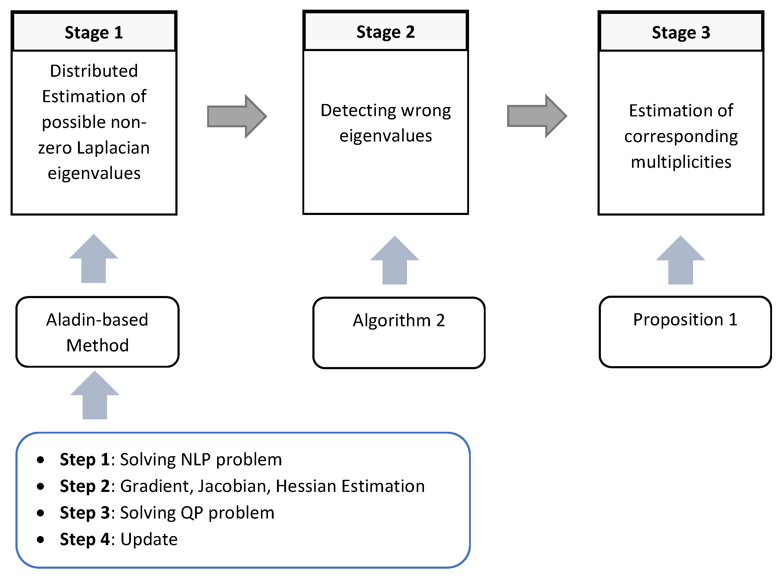
Section 3. The structure of this section can be illustrated as in
Figure 1. Before concluding the paper, the simulation results are described in
Section 4 to evaluate the efficiency of the proposed method.
3. Distributed Estimation of Laplacian Spectrum
Given an initial input-output pair
, with
, the matrix factorization problem (
3) is equivalent to minimize the cost function
that can also be rewritten as follows:
where
D is the number of steps before reaching average consensus and
.
Note that there is no need for a central node to set the initial input-output pair. Indeed, such a pair can be obtained after running a standard average consensus algorithm. Each node keeps in memory its own initial value and the consensus value.
Solving this factorization problem consists in finding the sequence of stepsize
. It is obvious that
are global parameters. To relax these constraints, define the factor matrices as
, where
,
,
. The problem above can be reformulated as a constrained consensus problem, that is to compute the sequence of stepsize
so that
. Moreover, in
Section 2.1,
D is denoted as number of non-zero distinct Laplacian eigenvalues. However, in this work, Laplacian matrix is assumed to be not-known in-a-priori. Therefore, the authors have assigned
D as
since
N can be estimated in the configuration step through the Random Walk Algorithm proposed in [
20]. Furthermore, the Laplacian Spectrum estimation procedure is divided in following stages:
Stage 1: Distributed estimation of the set of non-zero Laplacian eigenvalues , composing of the set of D non-zero distinct Laplacian eigenvalues .
Stage 2: Eliminating the wrong eigenvalues in the set to obtain the set
Stage 3: Estimating the multiplicities corresponding to each eigenvalues in the set to achieve the whole Laplacian spectrum .
3.1. Distributed Estimation of Non-Zero Laplacian Eigenvalues
For distributively carrying out the factorization of the average consensus matrix as factors of Laplacian based consensus matrices, the idea is to minimize the disagreement between neighbors on the value of
while ensuring that the factorization of the average consensus matrix is achieved. Such a factorization is assessed by constraining the values of the nodes after
h iterations of the consensus algorithm to be equal to the average of the initial values:
or, it can be rewritten in the following form:
This optimization has been solved by applying Augmented Lagrange Method [
1]. However, the disadvantage of this method is the slow convergence rate due to the fact that it is a non-convex optimization problem. To overcome this unexpected issue, the authors have suggested an interesting variant by converting the non-convex function into the convex one. By that, the optimization can be easily and effectively solved by Alternating Direction of Multipliers Methods (ADMM) [
16,
27]. In this paper, we proposed a method that can solve a non-convex problem effectively by employing ALADIN method, which is described as following:
- (1)
Step 1: ALADIN solves in parallel a sequence of equality-constrained non-linear problems (NLP) by introducing an augmented variables
as follows:
where
are penalty parameter and multiplier of the equality constraint, respectively.
.
One thing to note here is that with the given initial information
, running a standard consensus algorithm can determine the average value
. In addition to that, the positive semi-definite scaling matrices
can be randomly initialized or even be an identity matrix
. In this optimization problem (
7), augmented variables
are introduced with respect to the constraint
. However, this NLP is to be solved to define the variables
, hence, the constraint
is going to be relaxed.
The solution
obtained from (
7) is then used to check the stopping criteria the the next steps of the ALADIN-based algorithm procedure with
k being an iteration of the optimization process. Herein, if
and
, then one can get
as well as the Algorithm stops.
- (2)
Step 2: The Gradients, Jacobian matrices, and Hessian matrices are estimated for the next quadratic programming (QP) subproblems the as follows:
- (3)
Step 3: Analogically to inexact SQP method, the QP problem is solved to find the
and the affine multiplier
as follows:
where
is the slack variable, introduced into the QP sub-problem to attenuate the numerical reasons when the penalty parameter
becomes large.
- (4)
Step 4: The final step is to update
:
This update rule is relevant to the full-size step where
for the steplength computation, which proposed in [
25]. Then, projecting
on the constraint
to derive
.
The steps are repeated until the stopping criteria is satisfied.
In order to derive the distributed algorithm, let us take a closer look at each step of the proposed ALADIN-based method.
3.1.1. Implementation of Decoupled Nonlinear Problems
Firstly, in order to solve the decoupled NLP (
7) for
, the Augmented Lagrange method is applied here. Hence, we introduce the Augmented Lagrange function with the Lagrange multiplier
and penalty parameter
as below:
The solution of this problem can be obtained by applying a gradient descent method iteratively:
where
b stands for stepsizes of the gradient descent method, which can be chosen by fix constants or be determined by deploying a line-search algorithms such as Wolfe Condition, Back-stracking, or Armijo ones in [
28], while
c dedicates for the penalty parameter of the Augmented Lagrange method.
Lemma 2. The derivatives of this Lagrange function (14) is obtained as follows:where , and , while and 3.1.2. Implementation of the Coupling Quadratic Programming (QP)
Now, we apply the Karush–Kuhn–Tucker (KKT) conditions for solving the quadratic programming (QP) (
11). The Augmented Lagrange Function is described as follows:
The KKT conditions, which are showed in the
Appendix B yields a system of equations as follows:
Solutions of this system of equations are
respectively in the equivalent matrix form as follows:
This linear system can be solved by any linear solver. One thing to note here is the adaptive parameter
. We can start with a quite small
and adapt it during the optimization progress to relax the coupling conditions.
3.1.3. Implementation of an ADMM-Based Algorithm
Now, the update steps (
12) and (
13) are executed. Since the achieved
have to agree with the constraint (
), we solve the following optimization problem:
To solve this optimization problem, an Alternating Direction Method of Multipliers (ADMM) in [
16,
27] can be employed by introducing an augmented parameters
. Hence, the optimization can be rewritten as follows:
The Augmented Lagrange Function is defined as follows:
The ADMM solution acts in three steps repetitively until the tolerance achieves:
Lagrange multiplier update:
Herein, p is a iteration of the ADMM optimization process, then this output of this process is .
The distributed algorithm is illustrated in Algorithm 1.
The convergence analysis of the ALADIN method has been studied clearly for both non-convex and convex optimization problem in [
25]. Lemma 3 in [
25] has been proven that with the cost function
being twice continuously differentiable and letting
for
of problem (
5) be a regular KKT point. On the other hand, the Hessian
obviously, since
. There exists constants
such that for every point
satisfying the condition convergence of the decoupled minimization problem (
7) have unique locally minimizers
that satisfy
.
Moreover, if
when solving the QP (
11), with the (
) is a regular KKT point, then
. This is sufficient to prove local quadratic convergence of the algorithm as
are strictly positive constants. As a result, it is effectively applied to our proposed method since it is obviously an equality constrained non-convex optimization problem.
One thing to remark here is that in our study, the penalty parameters
can be updated using the following rules:
where
and
obtained by experience to avoid the numerical problem. Moreover, we can use the blockwise and damped Broyden–Fletcher–Goldfarb–Shanno (BFGS) update, which ensures positive definiteness of the
to preserve the convergence properties of ALADIN proposed in [
25].
3.2. Retrieving the Non-Zero Laplacian Eigenvalues
As stated before, the set of eigenvalues deriving from the Algorithm 1, denoted , composing of the set of non-zero distinct Laplacian eigenvalues .
Let
be the final consensus value reconstructed by
and the iteration scheme of the finite-time average consensus is implemented as in (
1). Following the idea of the Proposition 3 in [
27], we step-by-step assume to leave one element of the
, then, the remaining elements of this set are used to reconstruct
. If
is satisfied, then the left element is not the expected Laplacian eigenvalue. Hence, we can eliminate it out of the set
. Otherwise, the left element is one of non-zero distinct eigenvalues. We restore it in the set
and marked as an element in the set
. Now, the procedure is continued with another element to the end.
The distributed non-zero Laplacian eigenvalues are described in Algorithm 2.
| Algorithm 1. ALADIN-based Laplacian eigenvalues estimation |
Initialization:
Number of nodes N, tolerance , initial input-output pairs , where is retrieved from a standard average consensus algorithm. Each node initializes:
- (a)
random stepsizes for . - (b)
random Lagrange multipliers , for and . - (c)
Semi-positive definite matrices , learning rates b, penalty parameters .
Set ;
Repeat:
|
| Algorithm 2. Non-zero eigenvalues Estimation |
Input: set of stepsizes, obtaining form Algorithm 1 , the input-output pairs , the threshold . Set , . Repeat: While , pick an element out of , hence .
Construct average consensus iteration scheme from the remain stepsizes to determine as follows:
If , then and return to ( 3) If , then is included in and and return to ( 3)
Output: If is empty, then the non-zero distinct Laplacian eigenvalues can be derived by taking the inverse of the set ’s elements.
|
3.3. Multiplicities Estimation
Now, turning to the last stage, which is the corresponding Laplacian eigenvalues multiplicities estimation. In [
16], the authors have proposed a linear integer programming optimization problem to figure out the multiplicities:
Proposition 1 ([
16])
. Consider a connected undirected graph of N vertices with degree sequence and Laplacian matrix , having distinct non-zero Laplacian eigenvalues . Let be the vector of the corresponding multiplicities and be obtained by solving the integer programming below: The proof was given in [
16]. Since all the multiplicities
are positive integers, then Brand-and-Bound method has been deployed to derive
. Therefore, the problem (
24) can be rewritten equivalently in linear integer programming form as follows:
The Algorithm for this problem has been described clearly in [
16]. At this step, the whole Laplacian spectrum
has been obtained.
In fact, the estimation problem can be converted into a convex form and can be solved effectively by using ADMM-based method proposed in [
16]. However, the purpose of this study is extremely appropriate for non-convex optimization problem through deploying the promising ALADIN-based method.
4. Simulation Results
In this section, the efficiency of the proposed ALADIN-based method to estimate the Laplacian spectrum is evaluated by considering the two following case studies.
Firstly, it can be said that the Laplacian spectrum can decide the performance of the network since it reveals the connection of the network. For example, the robustness of the network can be estimated before starting the operations to avoid the interruption during these operations and, as a result, enhance the benefits technically and economically.
On the purpose of monitoring the connection of a large network
, one may face with the numerical issue in step 3 of the ALADIN-based method to solve the linear system (
19) due to the huge dimension of the obtained matrix that leads to the common ill-conditioning problem with the inverse matrix calculation.
In [
16], the authors have suggested to partition the large network into
M disjoint sub-networks
,
, [
29]. Let us define
and its cardinality
as the set of neighbors of node
i and its degree in
, respectively. Each sub-network is monitored by a super-node
i which knows the number
of agents in the sub-network and the associated average information state
. Node
is a super-node if it has at least one neighbor in a different subset, i.e.,
s.t.
. Let us consider that two sub-networks are connected if there exist edges linking at least two agents of these sub-networks. If two sub-networks are connected then their super-nodes are linked as showed in
Figure 2. Here, the network can be social network, power system network, molecular network, etc.
Let
be the undirected graph representing a network with
super-nodes, which are black nodes in
Figure 2.
G captures the interaction between sub-networks of
. Therefore, the large network is to be robust if the partitions are strongly linked to each other and if the critical threshold is high enough in [
16]. Then, the Laplacian spectrum of network of super-nodes
G can monitor the connection of the large network
via the robustness index.
4.1. Case Study 1
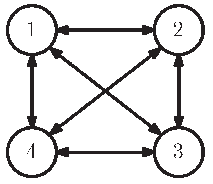
Let us consider a large network partitioning into 4 disjoint sub-networks. Each sub-network has only one super-node. These super-nodes interact with each other by the graph
, depicted in
Figure 3.
This network does have the Laplacian eigenvalues
. With the parameter of each super-node, denoted as
, after deploying Algorithm 1, the set of
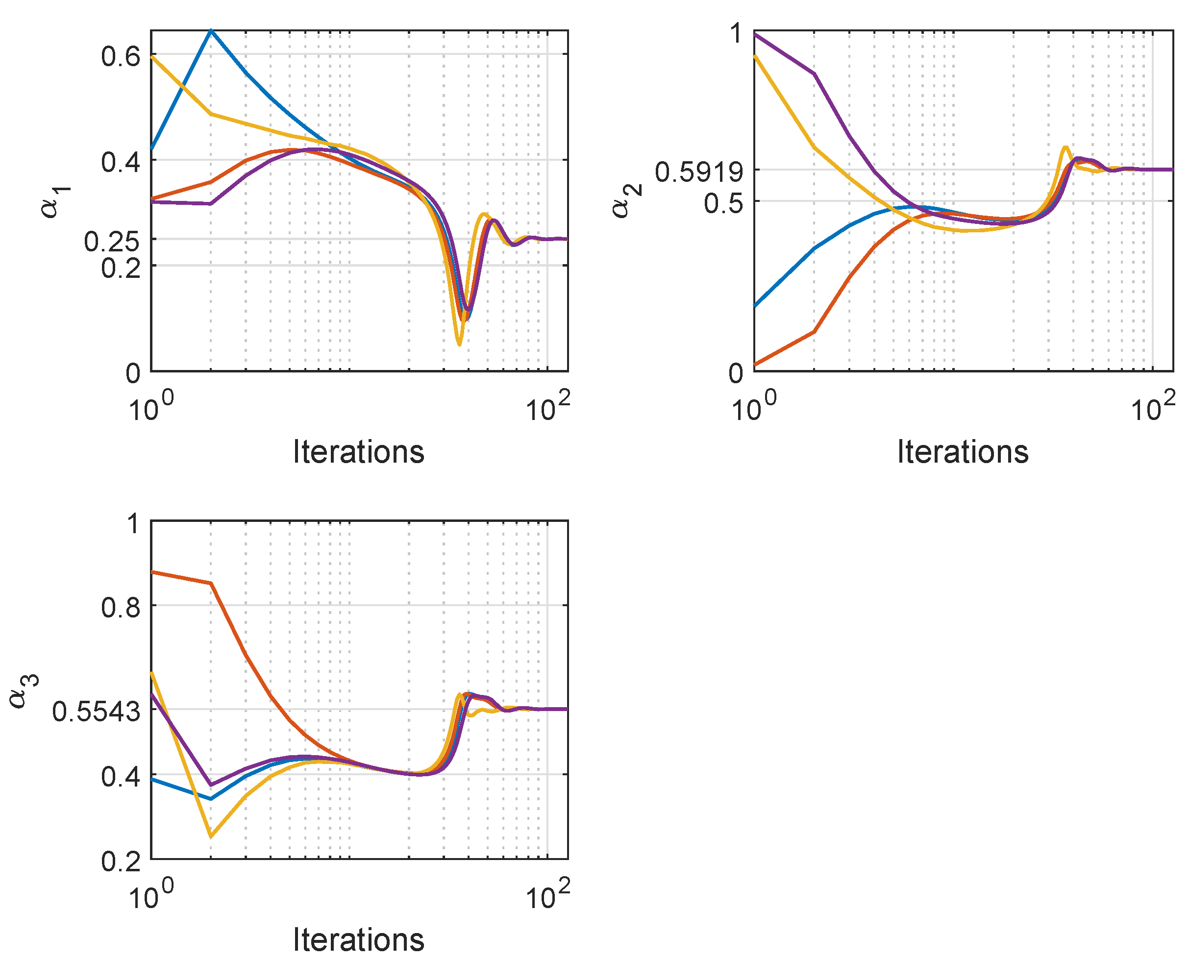
is obtained. The nodes trajectories are described as in
Figure 4.
As can be seen, all execute the consensus problem at the beginning of the procedure, and then dig into satisfying the constraint.
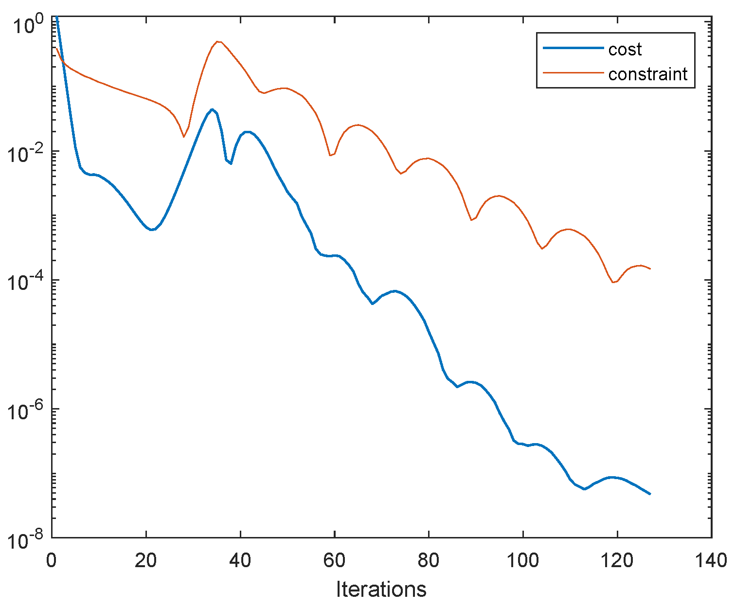
Figure 5 illustrate the convergence of the cost function
in according to the constraint
.
Furthermore, the Algorithm 2 is applied to eliminate the unexpected eigenvalues. As a result, we receive only one eigenvalue . In order to accomplish the Laplacian spectrum estimation’s procedure, we make use the Proposition 1 to pick out . Now, the entire Laplacian spectrum is achieved.
At this step, the robustness index such as Kirchhoff index or the number of spanning trees can be calculated.
Now, let us see how the proposed procedure works via the table below.
Table 1 is obtained after executing the proposed procedure.
As can be seen in
Figure 4, at the iteration of around 90 the procedure can be stopped. In order to access the robustness of the whole large network, it is necessary to define the critical threshold, introduced in [
16].
Next, we implement a comparison with the Lagrange method described in [
1] by considering Case study 2.
4.2. Case Study 2
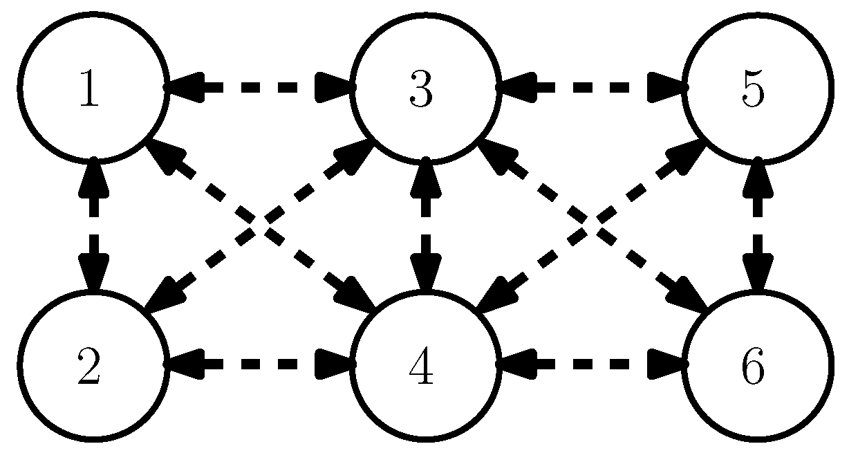
Let us consider a 6-node network described in
Figure 6.
It is known that for this topology, the Laplacian spectrum is .
Let us define the same initial information state of each node at time
:
for both methods. By using a standard consensus algorithm [
26], the consensus value
can be easily inferred.
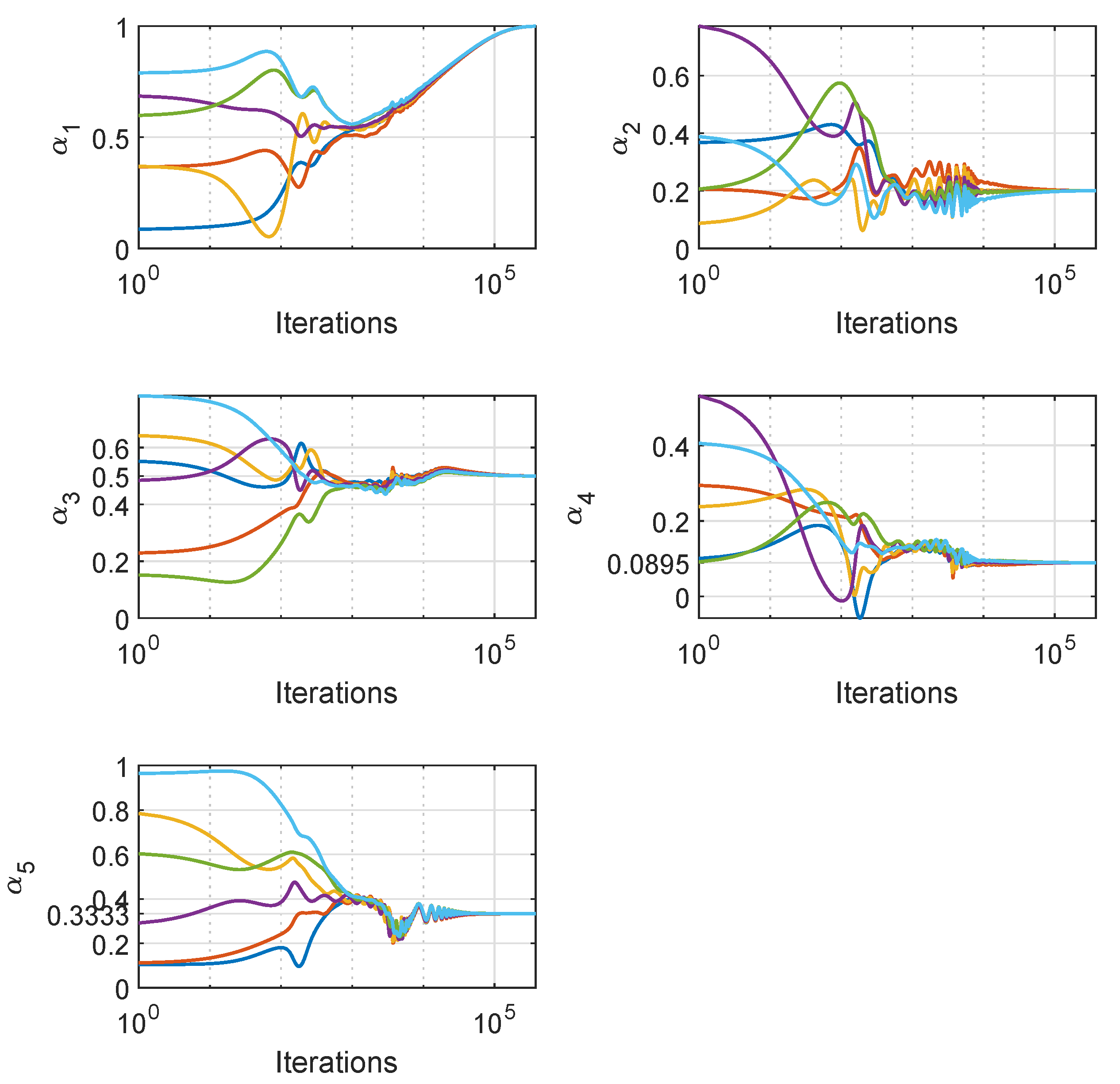
It can be seen in
Figure 7 that the Lagrange-based method in [
1] takes a long time to achieve the consensus first and then track the constraint to obtain the stepsizes
.
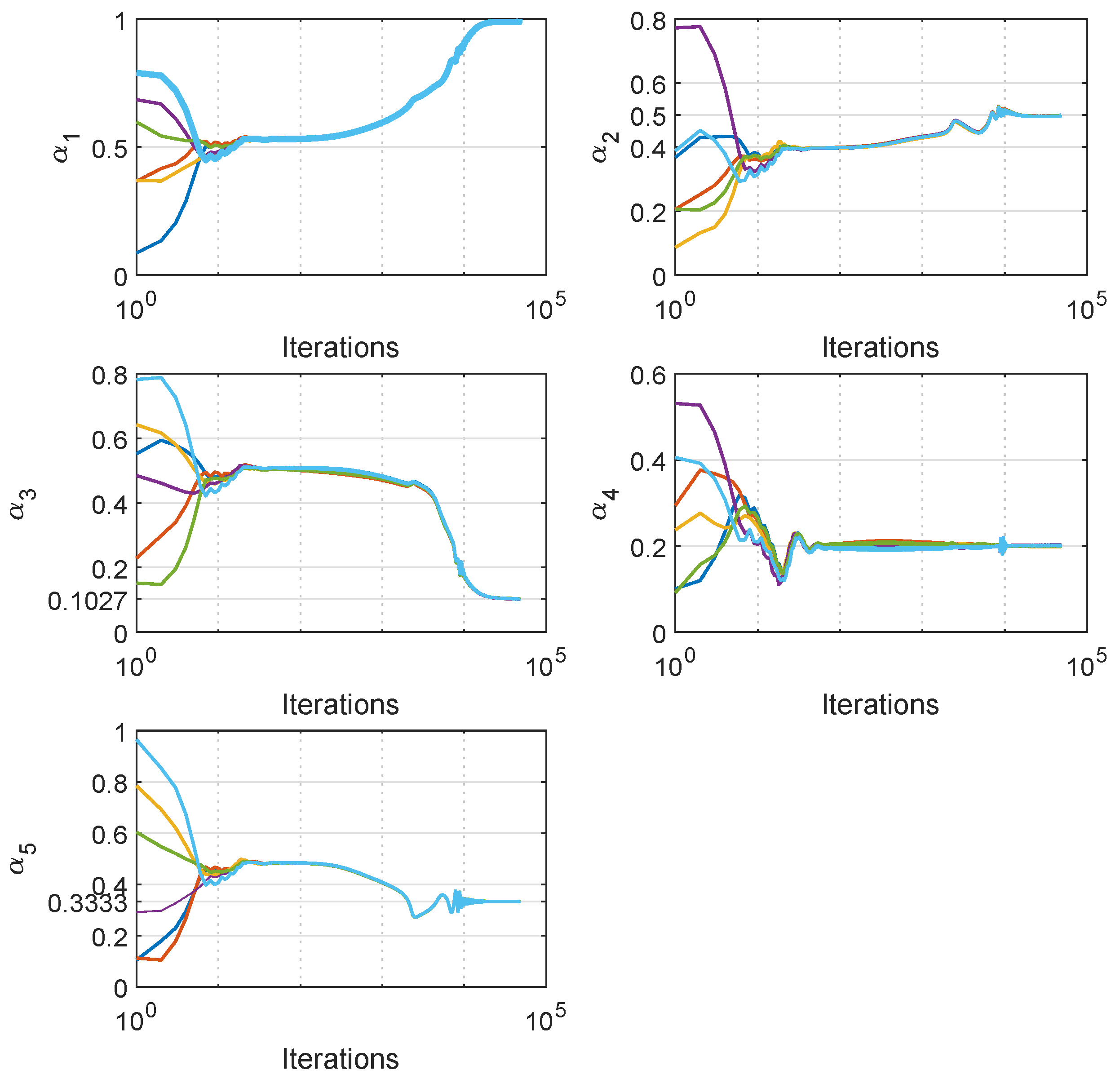
Now, with the same initial
, for the iterative procedure of the proposed method, the
after using the Algorithm 1 with the convergence trajectories of the
are illustrated in
Figure 8.
Figure 7 and
Figure 8 express the significant pros of our proposed method since the number of iterations is much less than that of Lagrange-based method. The consensus term is executed in advance from the start of the procedure and then try to reach the constraint term to figure out the expected values of the stepsizes
. Obviously, since the authors operate the proposed algorithm with the number of
being
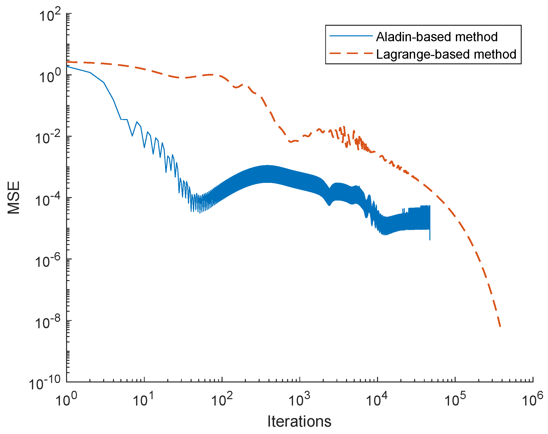
, it is needed to run the next stage to eliminate the residual values. As can be seen clearly, the executive time for ALADIN-based method is significantly faster than the proposed method as showed in
Figure 9.
Figure 9 shows that the ALADIN-based method approaches the destined values earlier than Lagrange-based method. Furthermore, in order to get the non-zero Laplacian eigenvalues of the given network, the Algorithm 2 is carried out to obtain vector of stepsizes
.
Finally, by constructing the Brand-and-Bound based method to solve the Problem 1, which has been proposed in [
16], we achieve the vector of multiplicities
, hence deduce the Laplacian spectrum
.
Now, let us see how the proposed procedure works via the table below.
Table 2 is obtained after executing the proposed procedure and the Lagrange-based method.
Notice that the proposed method gives results much better than the Lagrange-based method. Let us see that at the iteration of 33,950, the Lagrange-based method gives the set of that has still not satisfied the constraint.
Recently, besides the Laplacian spectrum estimation basing on the optimization approaches, there are also some works that approximate the Laplacian spectrum via iterative dynamics process (taking random walk for an example). However, from our point of view, the dominant contribution of our proposed method is the possibility of implementation in a decentralized manner. Moreover, another method to faster the convergence rate of the Laplacian spectrum estimation procedure is the ADMM-based method, proposed in [
16]. The important step in this work is to re-parameterize adequately the non-convex formulation into convex one. It is hard to compare the efficiency between ADMM-based method and the proposed method. Since, our study focuses on the non-convex formulation.
