Numerical Verification of Interaction between Masonry with Precast Reinforced Lintel Made of AAC and Reinforced Concrete Confining Elements

Featured Application

The described numerical model is intended for analyses of stress states and deformations of precast reinforced lintels made of autoclaved aerated concrete (AAC) bonded with AAC masonry and reinforced concrete confining elements.

Abstract

This paper describes results of numerical analyses of reinforced lintels made of autoclaved aerated concrete built into unconfined walls and walls confined with reinforced concrete. The combination of the Menétrey–Willam elastic-plastic failure criterion (M-W-3) and the Rankine criterion was used for numerical analysis of masonry. The parameters were determined by laboratory tests. Rebars were modelled using the Huber–Mises–Hencky yield criterion. The numerical model included interface elements att the interface between masonry units, at interfaces between reinforced concrete and masonry, and at interfaces between elements of test stands with a model using the Coulomb–Mohr (C-M) criterion. The majority of parameters of interface elements were assumed from laboratory tests. Results of numerical analysis were compared with laboratory tests. Results of numerical analysis and experiments were compatible in the range of load-carrying capacity of models and the failure method.

1. Introduction

Numerical analyses using the finite element method (FEM) present a wide range of possibilities for analysing structures composed of various materials, e.g., reinforced concrete or masonry [1,2,3]. Analyses often include load-carrying capacities of structures and their damage [4,5,6,7], stresses and deformations in zones of concentrated stresses [8,9,10], adhesive strength and anchorage of reinforcement [11,12,13], behaviour of superficial strengthening [14,15], effects of contraction deformations and creeping [16], effects of temperature on ageing mass concrete constructions [17], flows of heat and moisture flux [18,19], and new structural and material solutions [20]. Despite the significant progress in knowledge and continuously increasing processing power of computers, it is still impossible to build a numerical model for the global analysis of all physical effects taking place in built, ageing, and used constructions. For that reason, some simplifications are introduced to the models by adjusting them according to the planned computational objectives, the available information on the modelled material, and the processing powers of the software applied in the calculations.

The detailed numerical analysis of multi-material constructions is complex, because it requires the determination of many material parameters. Determination of the failure surface requires many tests under uniaxial or complex load states [21,22,23,24,25]. Apart from preparing the material model of failure, many parameters are required to describe effects observed at the interface of bonded materials, e.g., reinforcement and concrete and masonry units and mortar. Appropriate modelling requires specific contact elements, of which the parameters are taken from laboratory tests [8,22,26].

The aim of the tests performed in this study was to determine the interaction of autoclaved aerated concrete (AAC) lintels with brickwork above them, as well as the effect of confinement on the behaviour of walls under axial compression. The main purpose of numerical calculations was to diagnose the stress state in the masonry wall, comparing relationships between load and displacement, and those between crack morphology in the masonry and the lintel, using the masonry micro-model with advanced non-linear material models implemented into ATENA software.

This paper describes results from numerical calculations for reinforced lintels made of autoclaved aerated concrete, bonded with the masonry wall made of autoclaved aerated concrete, reinforced concrete tie beams and cores. The used material models of concrete, autoclaved aerated concrete, reinforcement and contact elements were based on material tests. Results from numerical calculations were compared with laboratory tests conducted on parts of walls containing the lintel and the tie beam, as well as full-scale walls.

2. Laboratory Tests

Laboratory tests were performed on compressed parts of walls containing reinforced lintels made of autoclaved aerated concrete (14 models with varied quantity of masonry layers above the lintel) and six full-scale walls under compression—two unconfined models. Two peripheral confining models and two models with inner peripheral confinement at the opening were used. Test procedures and results are described in detail in [27,28,29]. The research programme is presented in

Table 1. Research programme for parts of walls with lintels (dimensions in cm).

Element Name	Model Drawing	Model during Tests	Number of Models
1	2	3	4
N1			4
N2			4
N3			6

and

Table 2. Research programme for full-scale walls (dimensions in cm).

Element Name	Model Drawing	Model during Tests	Number of Models
1	2	3	4
MNSO			2
MSO			2
M2SO			2

.

Models were prepared of autoclaved aerated concrete blocks with strength f_b equal to 4.04 N/mm², thin-layer mortar with compressive f_m equal to 6.1 N/mm², and concrete, to obtain confined elements with mean compressive strength f_c,cyl = 25.5 N/mm². The tie beam reinforcement was composed of four steel rebars with a diameter of 10 mm, a material yield strength of 500 N/mm², and the ductility class C. Stirrups of rebars of 6 mm in diameter, made of the same steel, were at a spacing of 200 mm. Precast lintels were made of autoclaved aerated concrete with a strength f_c equal to 3.71 N/mm². They were reinforced with U-shaped meshes composed of rebars having a diameter of 8 mm, made of steel with a yield strength of 500 N/mm² and ductility of class A. The lower layer of the precast reinforcement was made of three rebars, and transverse reinforcement was at a spacing of 150 mm. The models were loaded by actuators with the operating range of 1000 kN (reading accuracy ± 1%) through steel spreader beams. The tendon system for loading was additionally used for the wall models. During the tests, applied load and displacements of the models were recorded by linear variable differential transducers (LVDT, reading accuracy ± 0.002 mm) and the non-contact optical system (DIC) using the ARAMIS 6M system by GOM company (the class of reading accuracy for displacements was ± 1%) [30].

3. Material and Numerical Models

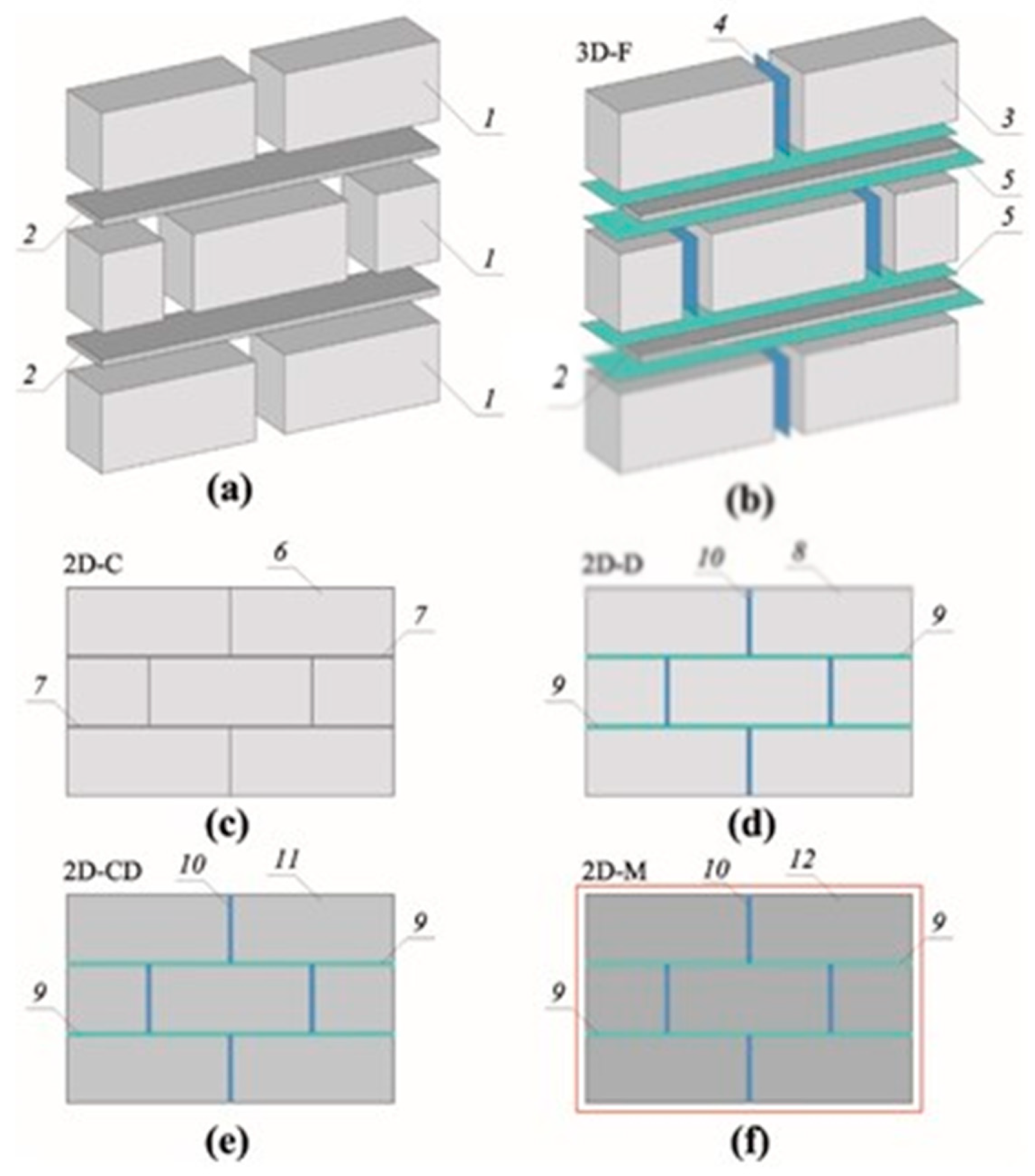
3.1. General Comments and Strategy Employed for Masonry Modelling

Numerical analysis by FEM is used to observe the behaviour of the structure in the linear stage, through cracking until complete loss of strength [31]. Non-linear material models are mainly used in numerical analyses. Models based on empirical observations differ in constitutive laws. Strength parameters can be defined for components of the masonry or the equivalent material by averaging properties. Hence, a few modelling methods can be identified for the numerical analysis of masonry structures by FEM. They are:

(a)

The macro-model, which treats the masonry structure as a material having identical mechanical parameters. Such a model is applied in practical computations for large masonry structures (finite elements can include two or more masonry units) [31,32,33,34];

(b)

The mezzo-model—a variant of the macro-model that is similar to the periodic micro-structure, which includes non-linear relations between mean stresses and mean deformations of the element, composed of masonry units and mortar layers equivalent to a given medium (of the same dimensions). Its basic element (representative volume element [35]) contains the required geometrical and physical information about any type of component for the masonry elements [36,37];

(c)

The micro-model, which identifies the masonry structure as a heterogeneous material. Classification into finite elements is made for each material (mortar, masonry unit). Different non-linear behaviour is assumed for bricks and mortar, including potential interaction forces between them. This type of model is usually used to analyse small constructions or to perform in-depth analysis. Its description requires information about the characteristics of components and the contact between them [22,32,33,34,35,36,38,39,40].

Taking into account the purpose of this paper—that is, observation of conditions in the masonry and the lintel and their interactions—the masonry wall (Figure 1a) was replaced by the masonry micro-model. In this case, there were a few methods of modelling. Alfaiate et al. [41] demonstrated that micro-models of walls can be prepared using 3D (Figure 1b) and 2D techniques for analysis of plane stress (e.g., plane deformations; connections between walls are less frequently used), as illustrated in Figure 1c–f. The main principle of micro-models, as illustrated in Figure 1d–f, is adding contact (interface) elements, which represent delamination at the interface between masonry units and mortar, to bed joints. We assumed that this type of modelling was the most adequate for the effects observed in our studies. Micro-modelling by the 3D technique was abandoned due the size of tested elements (Figure 1b). The second aspect taken into account when choosing the technique of micro-modelling was a series of cracks that developed in the masonry units during the tests, and the non-linear relationship between stress and deformation. Therefore, the authors decided not to use the model with linear and elastic masonry units (Figure 1d). The 2D micro-model, shown in Figure 1f [40], was chosen. Its masonry units took the mean mechanical parameters of the wall, then contact elements representing the behaviour of bed and head joints were placed at the interface of masonry units. All elements were modelled under conditions of plane stress. The reinforcement micro-model was also used for AAC lintels. Rebars were modelled as elements of non-linear parameters. Rebars were bonded with the surrounding AAC material, neglecting adhesion aspects.

3.2. Material Models

Material models were used in calculations to analyse the plane and spatial stress states: the elastic-based degradation model (the SBeta Material model) for concrete in confining elements, and the elastic-plastic based degradation model (the 3D Non-Linear Cementitious 2 model) for modelling the wall and the lintels [43]. Both models are usually used for brittle materials, and their boundary surface depends on mean hydrostatic stresses. The following material parameters were included in those models:

• Non-linear behaviour under compression, including hardening and softening
• Material cracking resulting from tension, based on non-linear mechanics of cracking
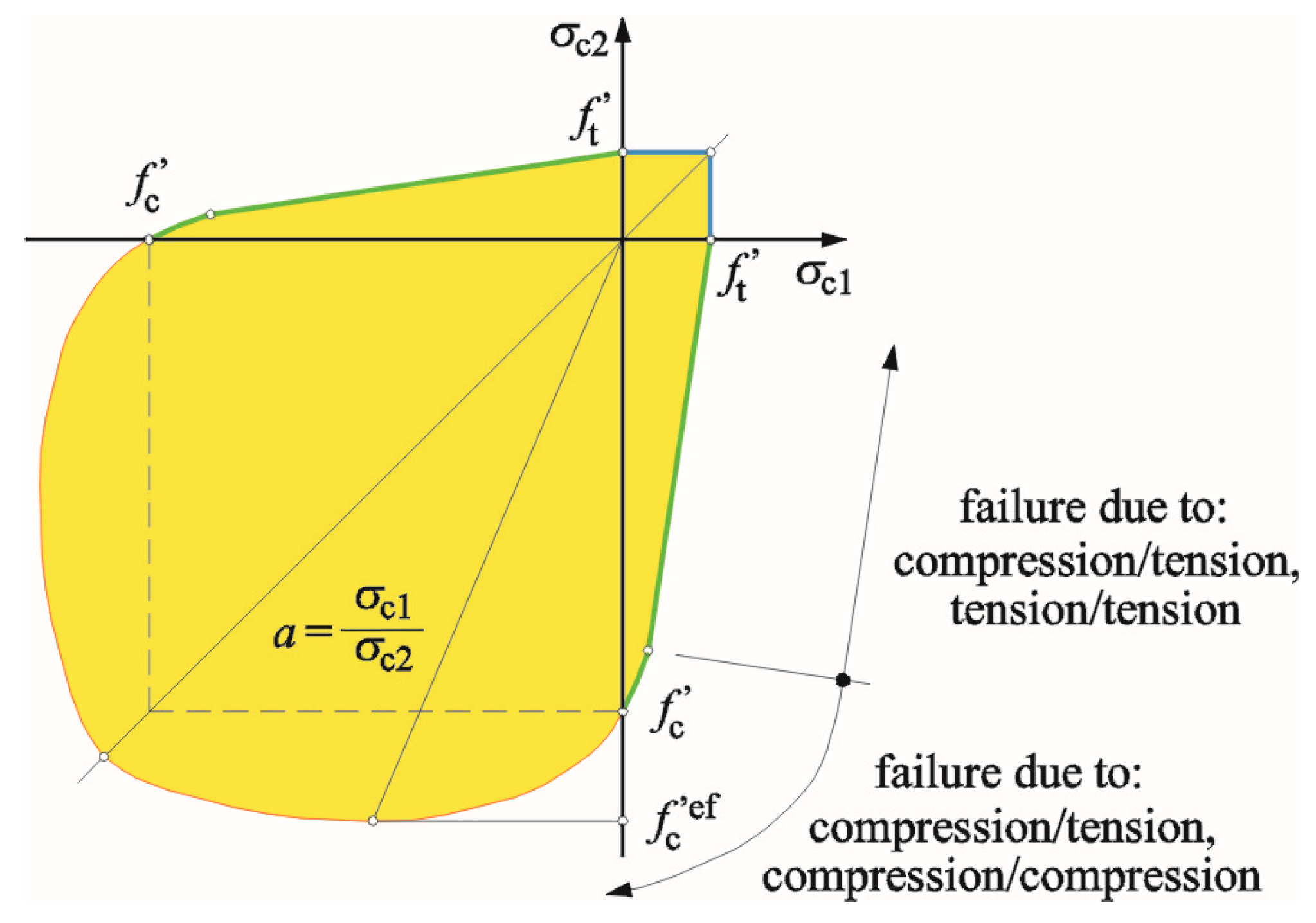
• Defined failure criterion for the material exposed to biaxial compression
• Softening of the material due to tension
• Reduced stiffness of the wall after cracking
• Possible modelling of cracks with set or changeable direction

3.2.1. Model of Concrete in Confining Elements—Elastic-Based Degradation Model

Principles of the continuum damage-based method were used to describe the development of damage in the discussed model. Effective stress expressed the non-linear behaviour of the material ${\sigma }_c^{\mathrm{ef}}$. Effective stress should be understood as stress under which deformations of the undamaged body are equal to deformations of the body damaged by true stress, described as equivalent strain ${\epsilon }^{\mathrm{eq}}$, calculated from the following relation [42]:

$${\epsilon }^{\mathrm{eq}}=\frac{{\sigma }_{ci}}{E_{ci}}$$

(1)

Effective uniaxial strain is regarded as deformation caused by stress ${\sigma }_{ci}$ and modulus of elasticity $E_{ci}$ in the i-direction, represented by damage and caused by stress related to stress direction ${\sigma }_{ci}$ [40]. A diagram of relationships between equivalent uniaxial stress and strain is shown in Figure 2 [41].

In a tensile state before cracking (range 1; Figure 2), material exhibited linear-elastic behaviour. Elasticity modulus $E_c$ is the initial modulus of material elasticity, and effective tensile strength ${f_t^{\prime }}^{\mathrm{ef}}$ was determined on the basis of the criterion of material behaviour under biaxial stress state. The general stress is expressed by the following relationship:

$${\sigma }_c^{\mathrm{ef}}=E_c{\epsilon }^{\mathrm{eq}}, 0\le {\sigma }_c\le {f_t^{\prime }}^{\mathrm{ef}}.$$

(2)

In the post-cracking phase (range 2; Figure 2), the material’s behaviour was described in two ways:

• The model of fictitious cracks resulting from the cracking mechanics and the accepted rule for crack width,
• The model of local deformations of a material point.

In the model of fictitious cracks, an exponential relationship was applied, as shown in Figure 3, on the basis of [43].

In a compression state (range 3; Figure 2), the stress–strain relationship was adopted from the FIB (Fédération internationale du béton) Model Code [44] in the following form:

$${\sigma }_c^{\mathrm{ef}}={f_t^{\prime }}^{\mathrm{ef}}\frac{kx-x^2}{1+\left(k-2\right)x},$$

(3)

where $x=\epsilon /{\epsilon }_c,$ $k=E_o/E_c,$ ${\sigma }_c^{\mathrm{ef}}$ represents normal compressive stress in the material, ${f_t^{\prime }}^{\mathrm{ef}}$ represents the effective compressive strength of concrete, x signifies normalised strains, $\epsilon$ signifies strains, ${\epsilon }_c$ signifies strains corresponding to effective compressive strength $f_c^{, \mathrm{ef}}$, k is the shape coefficient (k = 1 representing a linear function, and k = 2 representing a parabola), $E_o$ signifies initial modulus of elasticity, and $E_c={f_t^{\prime }}^{\mathrm{ef}}/{\epsilon }_c$ is the secant modulus of elasticity. The shape of the function expressing the stress–strain relationship in a compressive state is presented in Figure 4.

The adopted non-linear stress–strain relationship took into account the material damage developed before maximum stress was reached (as opposed to the material with visible cracks). The linear stress–strain relationships (range 4; Figure 2) referred to the state after achieving maximum compressive stress ${f_t^{\prime }}^{\mathrm{ef}}$. Displacements after reaching the maximum compressive strength $f_c^{, \mathrm{ef}}$ were only observed in the load plane. Displacement was assumed to occur regardless of the specimen size. Such a hypothesis was verified for concrete. The criterion, adjusted according to the results of concrete testing by Kupfer [45], was applied under biaxial compressive state conditions (Figure 5). The equivalent compressive strength was expressed with the following equation:

$${f_t^{\prime }}^{\mathrm{ef}}=\frac{1+3.65a}{{\left(1+a\right)}^2}{f}_c^{\prime },$$

(4)

where $a={\sigma }_{\mathrm{c}1}/{\sigma }_{\mathrm{c}2}$, σ_c1 and σ_c2 are main compressive stresses, and $f_c^{\prime }$ is material strength under a uniaxial compressive state.

Under biaxial tensile stress, tensile strength was constant and equal to material strength and uniaxial tensile force $f_t^{\prime }$. For elastic material with degradation, the model of smeared cracks developing in a uniform direction was applied. The crack was assumed to develop towards main strains ε₁, with ε₁ = ε_t corresponding to tensile strength. The direction of crack development did not change during further loading.

Table 3. Parameters of the elastic-based degradation model used in calculations.

Parameter	Test Formula or Results	Concrete in Confining Elements and Tie Beams
Uniaxial compressive strength $f_c^{\prime }=f_{c,cyl}$, N/mm2	Obtained from tests on cylindrical specimens ø150 × 300 mm	25.5
Deformations corresponding to uniaxial compressive strength of concrete εc		1.682 × 10−3
Uniaxial tensile strength $f_t^{\prime }$, N/mm2	Obtained from “Brasilian Test” for cylindrical specimens ø 150 × 300 mm	2.32
Initial modulus of elasticity $E_c$, N/mm2	Obtained from tests on cylindrical specimens ø 150 × 300 mm	3032
Poisson’s ratio $\nu$		0.2
Fracture energy Gf, MN/m	Calculated from the relationship $G_f=0.000025f_t^{\prime }$	5.793 × 10−5
Weakening function at tension	Assumed softening described by the exponential function	exponential
Displacement wc under tension, m	Displacements were calculated from the equation $w_c=5.14\frac{G_f}{f_t^{\prime }}$	−5.0 × 10−4
Model of cracks	developing in uniform directions	fixed
Weakening under compression $w_d$	Assumed default value of displacement $w_d$	0.05 mm
Reduced compressive strength in the direction parallel to cracks	Assumed default value of coefficient c	0.8

presents material parameters for concrete in confining elements and tie beams, used for numerical calculations.

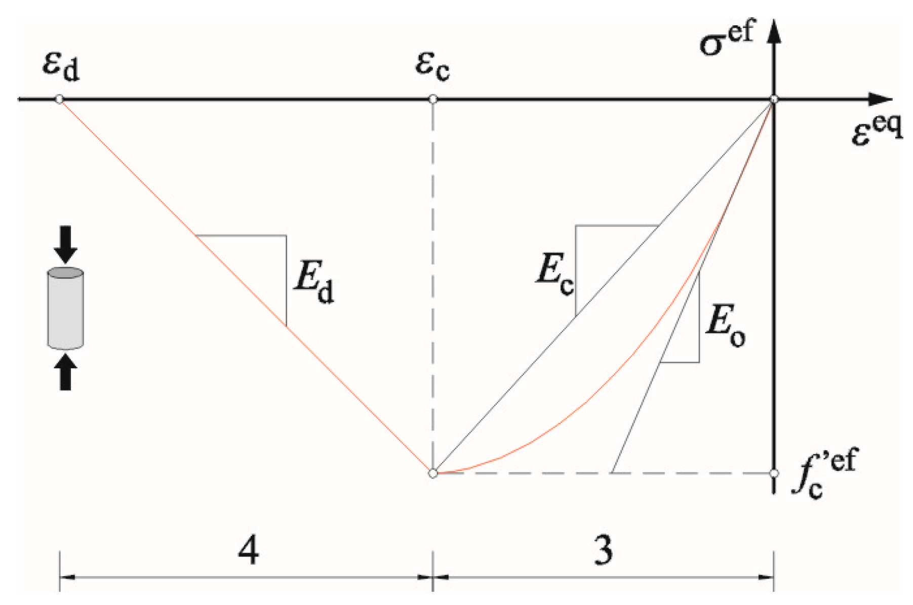
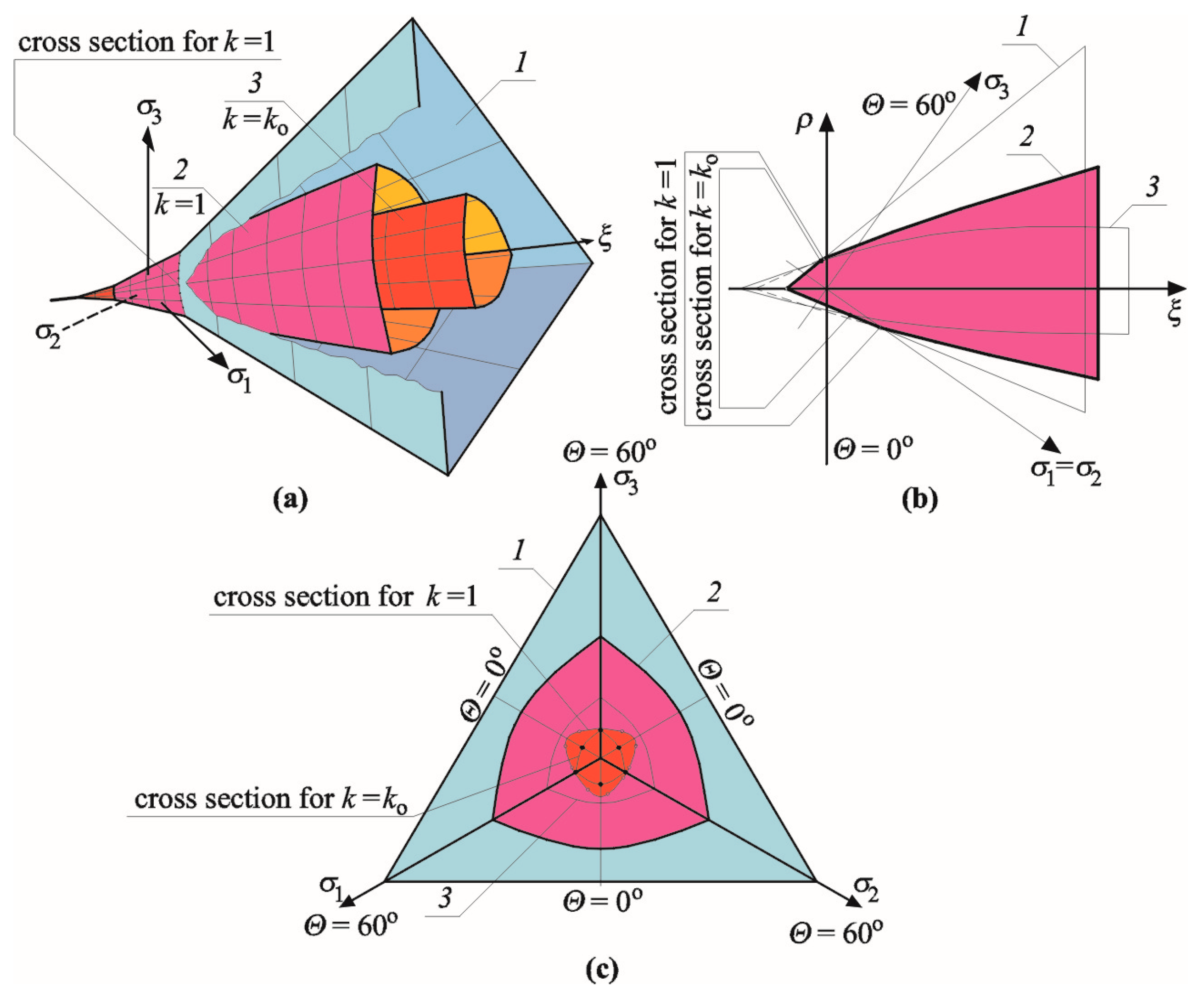
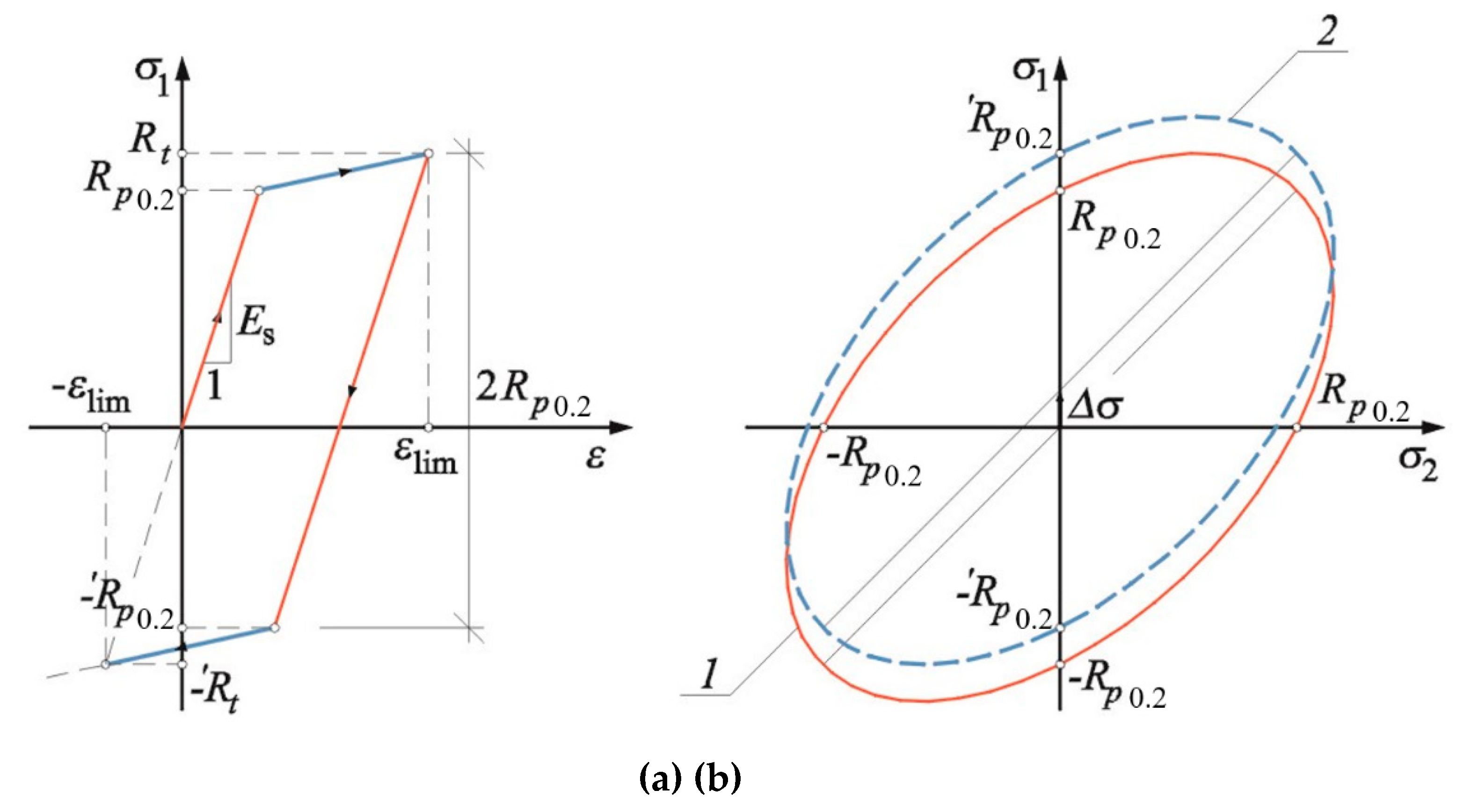
3.2.2. Model of the Wall and Lintels—Elastic–Plastic-Based Degradation Model

The degradation model of elastic–plastic material (3D Non Linear Cementitious 2) was a combination of the elastic–plastic and elastic–brittle models. The boundary surface model of Menétrey–Willam [46] is a modified version of the empirical model developed by Hoek and Brown [47] (used for rock description) changed by Weihe [48], who introduced the elliptic function of eccentricity e depending on the Lode angle Θ. The final form of a criterion used in that model was elaborated by Menétrey and Willam [46] who expressed a three-parameter yield surface M-W-3 as follows:

$$f^p\left(\xi ,\rho ,\Theta \right)={\left(\sqrt{1.5}\frac{\rho }{k\left(\kappa \right)f_c}\right)}^2+m\left(\frac{\rho }{\sqrt{6}k\left(\kappa \right)f_c}r\left(\Theta ,e\right)+\frac{\xi }{\sqrt{3}k\left(\kappa \right)f_c}\right)-c\left(\kappa \right)=0.$$

(5)

where

$$m=3\frac{{\left(k\left(\kappa \right)f_c\right)}^2-{\left({\lambda }_t{f}_t\right)}^2}{k\left(\kappa \right)f_c{\lambda }_t{f}_t}\frac{e}{e+1}$$

(6)

$$r\left(\Theta ,e\right)=\frac{4\left(1-e^2\right){\cos }^2\Theta +{\left(2e-1\right)}^2}{2\left(1-e^2\right)\cos \Theta +\left(2e-1\right)\sqrt{4\left(1-e^2\right){\cos }^2\Theta +5e^2-4e}}$$

(7)

where e represents the eccentricity of the elliptical function (Figure 6), assuming values from the range $e\in (0.5; 1.0)$; f_c and f_t signifiy uniaxial compressive and tensile strength, respectively; and λ_t ≥ 1 is the scaling parameter for the M-W-3 surface.

The boundary surface M-W-3 in the deviatoric section is composed of three tangential curves along compressive meridians (Figure 7), of which the shape is affected by the assumed eccentricity e of the elliptical function (Figure 6). When eccentricity e is 0.5, the deviatoric section of the failure surface is in the shape of an equilateral triangle. For e = 1.0, curves forming the deviatoric section take on the shape of circle. A curve, whose shape is similar to an ellipse, in the zone of biaxial compression values σ₁ − σ₂, σ₃ = 0, is a track of boundary surface in the plane of principal stresses. In the hydrostatic cross-section, the surface is formed by parabolic meridians intersecting at the tension point corresponding to triaxial tension. The ellipse extreme corresponds to material strength to biaxial compression f_bc. Concrete strength to biaxial stress was empirically determined as f_bc = 1.14f_c, and the corresponding eccentricity of the elliptical function was e = 0.52. For masonry units, the majority of tests covered solid brick [24,49]. The obtained values of solid brick strength to biaxial compression f_bc were within the range 1.02–1.14 f_c, and the corresponding eccentricity values were e = 0.501–0.511. In tests [40,42] conducted by the authors on silicate and AAC masonry units, the following e values were obtained: e = 0.504 (Ca-Si masonry units) and e = 0.52 AAC masonry units.

The behaviour of the material under tension was described using the Rankine criterion, the model of rotating smeared cracks or cracks developing in uniform directions, and the exponential function of softening. The Rankine surface is pyramidal (Figure 8) due to intersecting planes expressing the condition ${\sigma }_k\le f_t$, which in Haigh–Westergaard coordinates has the following form:

$$f^f=\xi -\sqrt{2}\rho \cos \Theta -\sqrt{3}{f}_t\le 0.$$

(8)

The parameter of surface adjustment λ_t > 1 determined the position of M-W-3 surfaces to the Rankine failure surface. At λ_t = 1, the plasticity surface of M-W-3 was always within the Rankine pyramid, and at λ_t = 2 the surfaces intersected at the plane of hydrostatic tension and minor compression. Figure 9 illustrates the relative location of boundary surfaces used in the elastic–plastic-based degradation model.

The required material parameters were obtained from the laboratory tests and validation of the model described in the paper [42].

Table 4. Parameters of the plastic and elastic model used in calculations.

Parameter	Test Formula or Results	Masonry	Lintel
Uniaxial compressive strength fb, N/mm2	Assumed from the tests	4.04	3.71
Plastic strain under compression εcp	Assumed from the tests	3.33 × 10−4	3.771
Uniaxial tensile strength fbt, N/mm2	Assumed from the tests	0.61	0.61
Initial modulus of elasticity Ec, N/mm2	Assumed from the tests	2204	2198
Poisson’s ratio ν	Assumed from the tests	0.200	0.179
Fracture energy Gf, MN/m	Assumed from the tests	1.07 × 10−5	1.602 × 10−5
Weakening function at tension	Assumed softening described by the exponential function	--	--
Displacement wc under tension [m]	Displacements were calculated from the equation $w_c=5.14\frac{G_f}{f_{tb}}$	4.36 × 10−4	--
Crack spacing smax [m]	Assumed constant value	0.5	0.5
Coefficient of tensile strength reduction at the softening phase cts	Assumed constant value for unreinforced material	0	0
Model of cracks	developing in uniform directions	--	--
Critical displacement under compression, m		−5.0 × 10−4	−5.0 × 10−4
Reduction of compressive strength caused by cracking fc-lim		0.8	0.8
Compressive stiffness of cracks sF		20.0	20.0
Size of aggregate particles [m]	Determined on the basis of macroscopic observations of the masonry units	0.02	0.02
Eccentricity of elliptical function e	Determined from the tests	0.5	0.5
Direction of plastic flow	Assumed as for incompressible material	β = 0	β = 0

presents material parameters for the wall and lintels used in numerical calculations.

Therefore, the stress state corresponding to tension and slight compression was expressed by the Rankine failure surface. The failure surface at higher compressive values of hydrostatic stresses was described by the M-W-3 surface. Displacement of the M-W-3 surface along the hydrostatic axis was caused by changes in the parameter λ_t. The surface could expand, simulating the stages of hardening or softening, depending on the parameter κ, related to dilatational, non-dilatational or plastic strains:

$$d\kappa =d{\epsilon }_v^p=d{\epsilon }_1^p+d{\epsilon }_2^p+d{\epsilon }_3^p.$$

(9)

A temporary shape and location of the M-W-3 surface at the hardening phase was defined by the hardening function (κ), which depended on the hardening/softening parameters [50,51]. The hardening function was directly included in the M-W-3 failure surface as a scaling factor of material compressive strength (f_c) and had the following elliptic form [43]:

$$k\left(\kappa \right)=k\left({\epsilon }_v^p\right)=k_o+\left(1-k_o\right)\sqrt{1-{\left(\frac{{\epsilon }_{\mathrm{v},\mathrm{t}}^p-{\epsilon }_v^p}{{\epsilon }_{\mathrm{v},\mathrm{t}}^p}\right)}^2},$$

(10)

where ${\epsilon }_{\mathrm{v},\mathrm{t}}^p$ is the plastic dilatational strain obtained from uniaxial compression test (the onset of softening), and k_o is the value defining the initial surface of plasticity that reduces the elastic state (the onset of plasticity), where ${\epsilon }_{\mathrm{v},\mathrm{t}}^p$ is the plastic dilatational strain obtained from the uniaxial compression (the onset of softening), and k_o is the value defining the initial surface of plasticity that reduces the elastic state (the onset of plasticity). At the end of the process, the function of reinforcement maintained a constant value, and the material came to the softening phase controlled by the softening function c, which simulated decohesion by shifting the yield surface towards the negative part of the hydrostatic axis. For the uniaxial compression, that function had the following form [43]:

$$c\left(\kappa \right)=c\left({\epsilon }_v^p\right)={\left(1/\left[1+{\left(\frac{n_1-1}{n_2-1}\right)}^2\right]\right)}^2,$$

(11)

where $n_1={\epsilon }_v^p/{\epsilon }_{\mathrm{v},\mathrm{t}}^p$ and $n_2=\left({\epsilon }_{\mathrm{v},\mathrm{t}}^p+t\right){\epsilon }_{\mathrm{v},\mathrm{t}}^p$.

Parameter t, describing the volumetric strain, controlled the slope of the softening function. The value of the softening function c made the value equal to 1 at the phase of reinforcement and equal to 0 at the complete softening phase of the material with decohesion. Changes in functions of strengthening k and softening c are shown schematically in Figure 10.

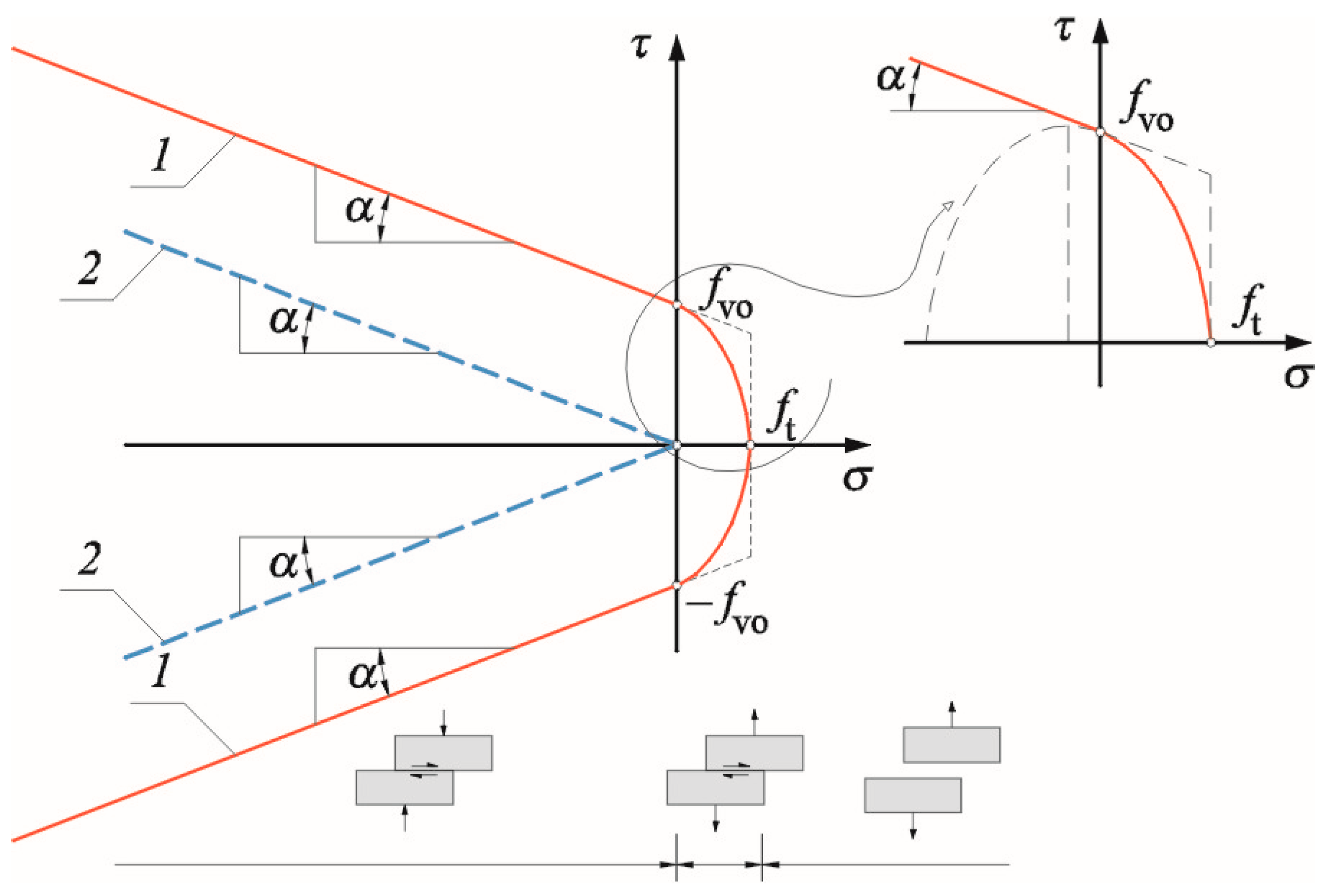
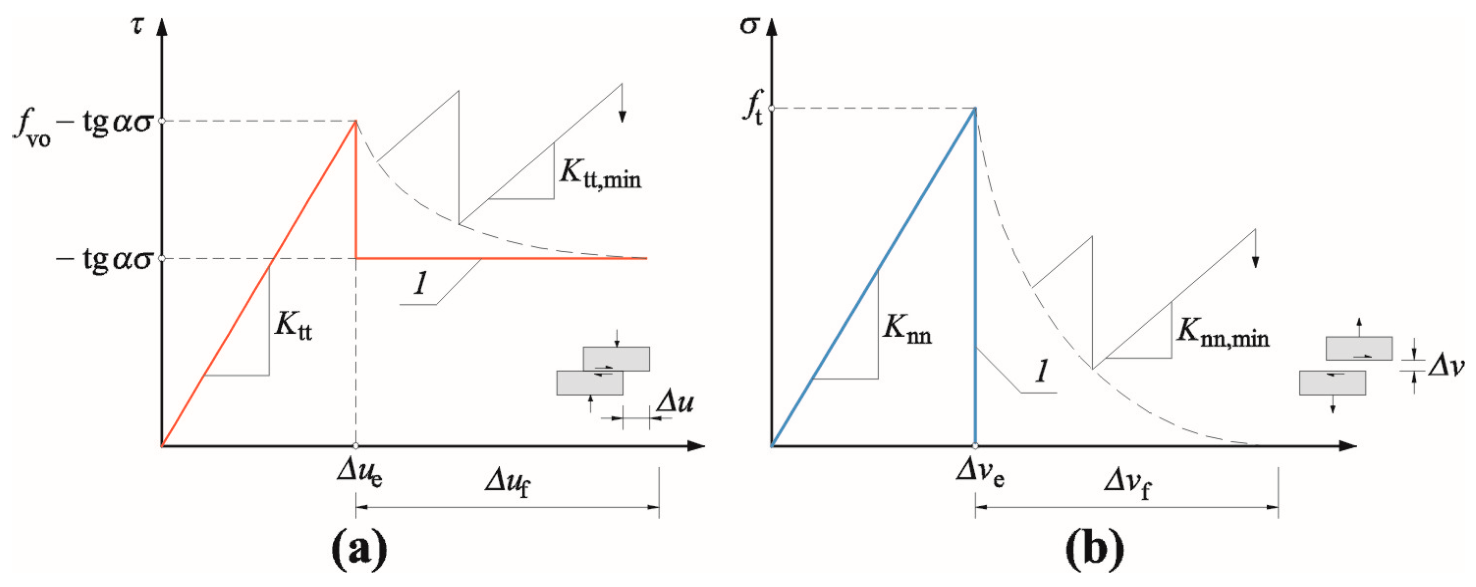
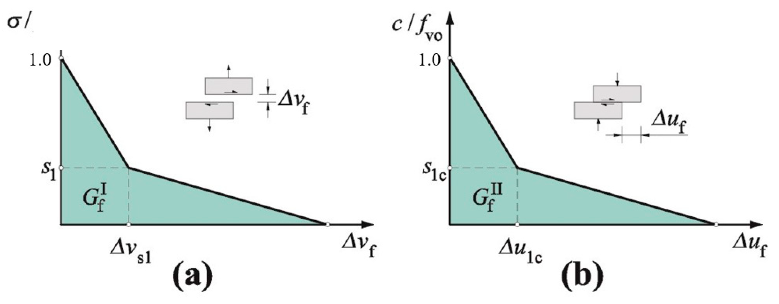
3.2.3. Model of Contact (Interface) Elements

Contact elements were used in the numerical models. They provided more accurate representations of the model behaviour and the accuracy of obtained results. The contact elements were applied at the interface between the masonry units in head joints, between the masonry units with mortar in bed joints, and between the masonry units and reinforced concrete and steel elements. The initial shear stiffness K_tt and the initial normal stiffness K_nn were decisive parameters for the contact elements. Constitutive relations for the flat state, regarding horizontal and standard displacements, were expressed in the following way:

$$\left[\begin{array}{l}\tau \hfill \\ \sigma \hfill \end{array}\right]=\left[\begin{array}{ll}{K}_{\mathrm{tt}}\hfill & 0\hfill \\ 0\hfill & K_{\mathrm{nn}}\hfill \end{array}\right]\left[\begin{array}{l}\Delta u\hfill \\ \Delta v\hfill \end{array}\right],$$

(12)

where τ = shear stress, and σ = normal stress.

The failure surface was expressed using the Mohr–Coulomb criterion (Figure 11) for normal compressive stresses (13) and elliptical cap at the side subjected to tension (14), in the following form:

$$\left|\tau \right|\le f_{\mathrm{vo}}-\mathrm{tg}\alpha \sigma , \mathrm{when} \sigma \le 0,$$

(13)

$$\begin{array}{c}\tau ={\tau }_o\sqrt{1-\frac{{\left(\sigma -{\sigma }_c\right)}^2}{{\left(f_t-{\sigma }_c\right)}^2}}, {\tau }_o=\frac{1}{\sqrt{1-\frac{{\sigma }_c^2}{{\left(f_t-{\sigma }_c\right)}^2}}}, {\sigma }_c=\frac{-f_t^2\mathrm{tg}\alpha }{f_{\mathrm{vo}}-2f_t\mathrm{tg}\alpha }\\ \mathrm{when}, 0<\sigma \le f_t.\end{array}$$

(14)

For normal stress greater than tensile strength, the criterion was expressed as

$$\tau =0, \mathrm{when} \sigma >f_t.$$

(15)

For shear stresses greater than limit values described by relationships (13) and (14), the boundary surface was reduced to the residual surface, corresponding to the dry friction surface described by the following equations:

$$\left|\tau \right|\le \mathrm{tg}\alpha \sigma \mathrm{when} \sigma \le 0,$$

(16)

$$\tau =0 \mathrm{when} \sigma >f_t.$$

(17)

A cap material was used in the interval of tensile stresses with the Mohr–Coulomb criterion replacing straight lines and with the ellipse intersecting the axis of normal stresses at the point corresponding to tensile strength f_t. The intersection point between the ellipse and the axis of shear stresses τ corresponded to cohesion c, and was tangential at that point to the Mohr–Coulomb line (Figure 11). Therefore, parameters of interface elements had to meet the following conditions:

$$f_t<\frac{f_{\mathrm{vo}}}{\mathrm{tg}\alpha },f_t<f_{\mathrm{vo}},$$

(18)

$$c>0,f_t>0, \mathrm{tg}\alpha >0.$$

(19)

The relationships of shear stress–displacement, and normal stress–displacement until achieving the failure surface by shear stress were linear, defined by the initial shear stiffness K_tt and the initial normal stiffness K_nn (Figure 12). Due to there being zero thickness of the contact elements, stiffness values should be greater than those of adjacent finite elements, but at the same time low enough to avoid numerical instability.

Additionally, stiffness values K_tt,min and K_nn,min were required to obtain numerical solutions for the softening phase. Values were chosen iteratively, decreasing initial stiffness values K_tt and K_nn. Multi-section relationships could be defined to describe the behaviour of the contact element subjected to tension and shearing. Two-section softening laws, shown in Figure 13, were the simplest solutions. Characteristic breaking points of curves were defined according to [52], from the following equations:

$$s_1=\frac{f_t}{4}, \Delta u_{1c}=0.75\frac{G_f^{\mathrm{II}}}{f_t}.$$

(20)

Apart from fracture energy $G_f^I$ determined under the axial tension and $G_f^{\mathrm{II}}$ at shearing, the softening laws depended on equivalent displacement, and were defined in the following way:

$$u_f^{\mathrm{eq}}=\sqrt{\Delta u_f^2+\Delta v_f^2},$$

(21)

where $\Delta u_f=\Delta u-\Delta u_e$ signifies non-elastic horizontal displacement, calculated as the difference between total $\Delta u$ and elastic displacements $\Delta u_e$, and $\Delta v_f=\Delta v-\Delta v_e$ signifies non-elastic vertical displacement, calculated as the difference between total $\Delta v$ and elastic displacements $\Delta v_e$.

That solution caused the cohesion degradation to have an impact on tensile strength, and vice versa. For example, when the bond was damaged by compression, tensile strength was also reduced. A typical behaviour of the contact elements in elastic and post-elastic phases caused by shearing and tensions is shown in Figure 12. The default behaviour of the contact elements was brittle (straight line) when the softening laws were not defined. In addition, default breaking of the curve and shear stress values reduced to the value of dry friction at shearing. Material parameters are presented in

Table 5. Parameters of contact elements taken for modelling autoclaved aerated concrete (AAC) walls.

Parameter	Test Formula or Results	Bed Joint	Head Joint
1	2	3	4
Normal stiffness Knn, MN/m	Calculated from the equation: $K_{\mathrm{nn}}=\frac{E}{a}10$ E—the greater of the elasticity moduli of adjacent materials; a—dimension of finite element $K_{nn}=\frac{E}{a}10$	1.02 × 106	1.02 × 106
Shear stiffness Ktt, MN/m	Calculated from the equation: $K_{tt}=\frac{G}{a}10$ E—the greater of the shear moduli of adjacent materials; a—dimension of finite element	4.51 × 105	4.51 × 105
Tensile strength fbt, N/mm2	Determined from tests	0.29	0
Cohesion fv0	Determined from tests	0.31	--
Friction coefficient tgα	Determined from tests	0.626	0.92
Normal stiffness Knn,min, MN/m	Calculated as 0.01 Knn	1.02 × 104	1.02 × 104
Shear stiffness Ktt,min, MN/m	Calculated as 0.01 Ktt	4.51 × 103	4.51 × 103
Fracture energy under shearing $G_f^{II}$, MN/m	Determined from tests	2.37 × 104	--
Displacement u1c, mm	Calculated from the equation:$\Delta u_{1c}=0.75G_f^{II}/f_t$	−6.13 × 104	--
Equivalent displacement $u_{eq}^f$, mm	Calculated from the equation: $u_{\mathrm{eq}}^f=\frac{4\left(2G_f^{\mathrm{II}}-f_t{u}_{1\mathrm{c}}\right)}{f_t}$	4.09 × 104	--
Weakening function at tension	--	Assumed default relationship acc. to Figure 3b
Softening function at tension	Assumed as for incompressible material	Assumed two-section relationship acc. to Figure 3a	Assumed default relationship acc. to Figure 3b

and

Table 6. Parameters of interface elements at the interface of the wall and reinforced concrete elements.

Parameter	Test Formula or Results	Bed Joint	Head Joint
1	2	3	4
Normal stiffness Knn, MN/m	Calculated from the equation: $K_{nn}=\frac{E}{a}10$	3.92 × 106	1.02 × 106
Shear stiffness Ktt, MN/m	Calculated from the equation: $K_{tt}=\frac{G}{a}10$	1.67 × 105	4.51 × 105
Tensile strength fbt, N/mm2	Assumed value as for the wall	1.5	1.5
Cohesion fv0		∞	∞
Friction coefficient tgα		∞	∞
Normal stiffness Knn,min, MN/m	Calculated as 0.01 Knn	3.92 × 104	1.02 × 104
Shear stiffness Ktt,min, MN/m	Calculated as 0.01 Ktt	1.67 × 103	4.51 × 103

.

3.2.4. Model of Reinforcement

The steel reinforcement was modelled with the Huber–Mises–Hencky yield surface, illustrated by Haigh–Westergaard coordinates as an infinitely long cylindrical surface (Figure 14) expressed by the following equation:

$$F\left(\rho \right)=\rho -\sqrt{\frac{2}{3}}{f}_t,$$

(22)

where f_t is the yield strength of steel.

The criterion, based on a bilinear relationship between stress and deformation, was used with the associated flow law and kinematic hardening law (Figure 14) that is usually adequate for metals and is known as the Prandtl-Reuss model (Figure 15). The applied law of kinematic hardening takes into account the change in orientation of the yield surface under compression due to tensile yield strength, that is, the Baushinger effect. Parameters of concrete steel in lintels, confining elements and tie beams are shown in

Table 7. Mechanical parameters of concrete steel used in the numerical model.

Type of Reinforcement and Dimensions of Rebar Cross-Section, mm	Parameter
	Es N/mm2	ν	Rp0,2 N/mm2	ET N/mm2	Rt N/mm2	εlim %
Longitudinal reinforcement in lintels (round rebars with a diameter of 8 mm)	198,000	0.3	520	245	544	9.9
Transverse reinforcement in lintels (round rebars with a diameter of 4.5 mm)	201,000		479	233	501	9.6
Longitudinal reinforcement in confining elements and tie beams (round rebars with a diameter of 12 mm)	179,330		616	242	644	11.9
Transverse reinforcement in lintels (round rebars with a diameter of 10 mm)	178,500		685	261	716	12.3

.

The models of materials and contact elements used were calibrated and verified by conducting numerical analysis of the wall models to determine the wall strength. The obtained results are described in [9,53,54,55]. The results, in the form of the relationship between the normal stress σ_y and horizontal ε_x and vertical deformations ε_x, were compared with experimental results. Initially assumed parameters of materials indicated that the results for maximum compressive stress were lower by 30% than the test results, and that the moduli of longitudinal elasticity were consistent. Such a big discrepancy in the failure stress led us to assume some material parameters corresponding to masonry units and replacement of bed joints with the contact elements. The calibration of material parameters consisted in using the reduction coefficient, equal to the ratio of the compressive strength of wall to the compressive strength of the masonry unit. For compressive strength values obtained from the tests, the reduction coefficient was equal to f_cm/f_b = 2.83/4.04 = 0.70. The results of the numerical calculations based on the corrected material parameters differed by no more than 2% from the experimental results. The wall analysis, with reference to deformability and crack morphology, also provided satisfactory results. The calibrated elastic–plastic model of the material with the failure surface was used for analysis in the subsequent phase.

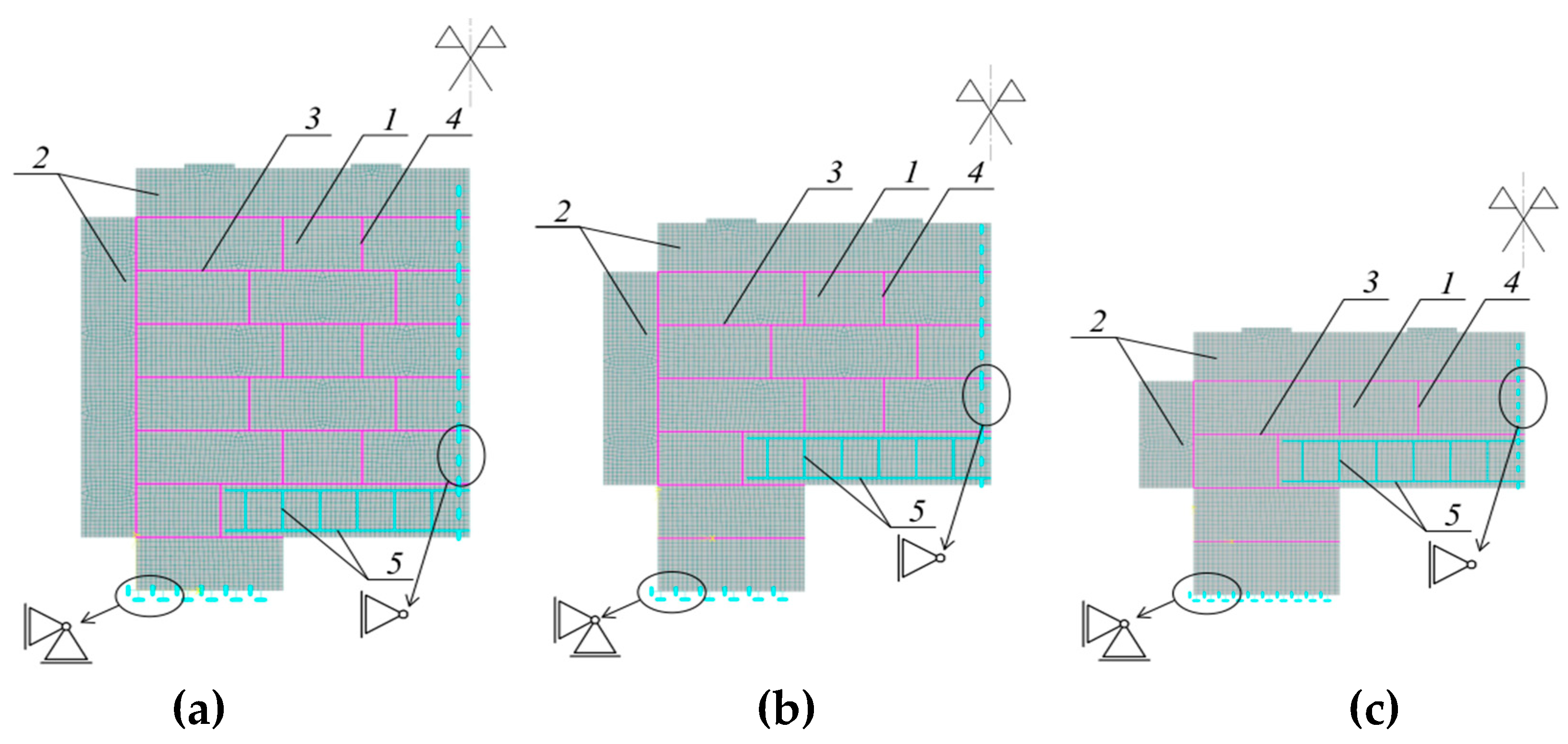
3.2.5. Numerical Models of Whole Walls and Their Parts

Numerical models were developed for each test model of the parts of full-scale walls using ATENA software [50]. The symmetry of the test models was used to model a half of the test model with steel elements of the test stand. The elastic–plastic model of the M-W-3 materials was assigned to masonry units and AAC lintels. Material parameters are shown in Table 4 (Section 3.2.2). The contact elements, with parameters shown in Table 5 (Section 3.2.3), were used in the bed and head joints, and between the wall and the tie beam. The elastic-based degradation material, with parameters specified in Table 2 (Section 3.2.1), was used for reinforced concrete elements. The Huber–Mises–Hencky (H-M-H) models, with parameters shown in Table 7 (Section 3.2.4), was used for steel reinforcement placed in the lintel. Four-node finite elements, with two degrees of freedom for each node and the plane stress state, were used to model the wall and the lintels. The side of each finite element had a maximum length of 20 mm. Reinforcement in AAC lintels, confining elements and tie beams was modelled using bar finite elements with one degree of freedom for each node. Total adhesion of reinforcement to adjacent concrete was applied. The models of wall parts were loaded in sequences during three phases corresponding to loading phases of the laboratory models. The load applied in phase I resulted from the self-weight of the model and elements of the test stand. The first loading stage was realized in the subsequent stage, that is, horizontal loads were transmitted through the prestressing tendon system on the models of wall parts, or vertical load was transmitted to the full-scale walls through tendons. In phase III, the models were loaded, that is, load from the spreader beams was applied. Loading was divided into steps in each phase: three steps in phase I, ten steps in phase II and an increase in the load by 1 kN until the complete loss of strength was brought about in the final phase. The numerical models of wall parts are shown in Figure 16, whereas the models of full-scale walls are illustrated in Figure 17.

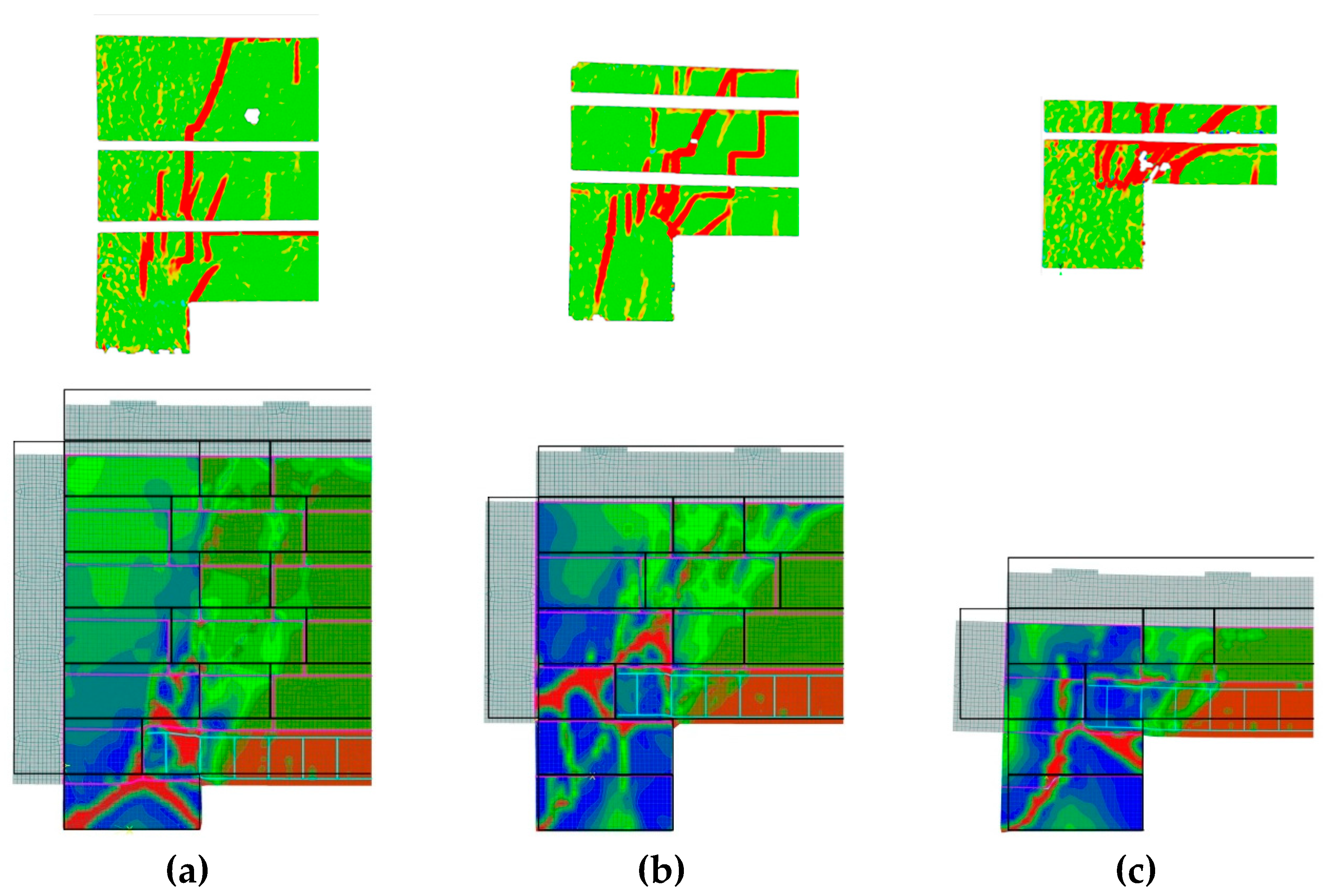
4. Results of Numerical Analysis

4.1. Parts of Walls

Results of numerical analysis and experiments were compatible in the range of the load-carrying capacity of models and the failure method. Images of damaged parts of the walls obtained with the non-contact optical system during the laboratory tests and the results of the numerical model at the failure phase are compared in Figure 18.

The maximum load of 444 kN and the corresponding deflection of 2.89 mm were reached in the first numerical model, NI. Destructive force at the level of 93% and lintel deflection at the level of 129% (2.9 mm) were obtained by comparing values from numerical calculations and mean values for the models of the NI series. First cracks were found at the lintel, above the support edge, under a load of 384 kN and a lintel deflection of 0.6 mm, which was 50% of the deflection and 94% of the load in the NI-1 and NI-2 test models. The lower convergence of results was found when those values were compared with models NI-3 I NI-4, for which the cracks were observed using the optical system. The calculated deflection and loading were respectively 333–375% and 392–469% of the values recorded during the tests.

For another numerical model, NII, the maximum load was 420 kN, and the deflection at failure was equal to 11.2 mm, which constituted 85% and 220% of mean values obtained from the tests. The first cracks in the numerical model developed at the support edge of the lintel, as in the case of the model with five layers of brickwork. The obtained cracking force was 312 kN and the corresponding deflection was 0.6 mm. When those results were compared with the mean values obtained for the tested models of the NII series subjected to optical analysis, the cracking force and deflection constituted 238% and 167% of the experimental values.

The smallest numerical model, NIII, was destroyed under a load of 376 kN and a deflection of 5.37, which constituted 85% of the loading force and 70% of the mean values from the tests. Cracking of the model developed simultaneously between the masonry units and at the support edge of the lintel. The force was 220 kN, which constituted 247% of the cracking force, and deflection was equal to 0.45 mm, which constituted 98% of the deflection determined by the tests. Figure 19 illustrates the relationship between loading and displacement of laboratory and numerical models.

By comparing the relationship between force-deflection, illustrated in Figure 19, deflection of the lintel obtained from the numerical model was found to be smaller than in the laboratory models. This was caused by difficulties in proper modelling of cracks. Cracks that appeared in the laboratory models became wider under an increase in loading, and consequently deflection increased. It is difficult to reproduce this effect using the numerical model.

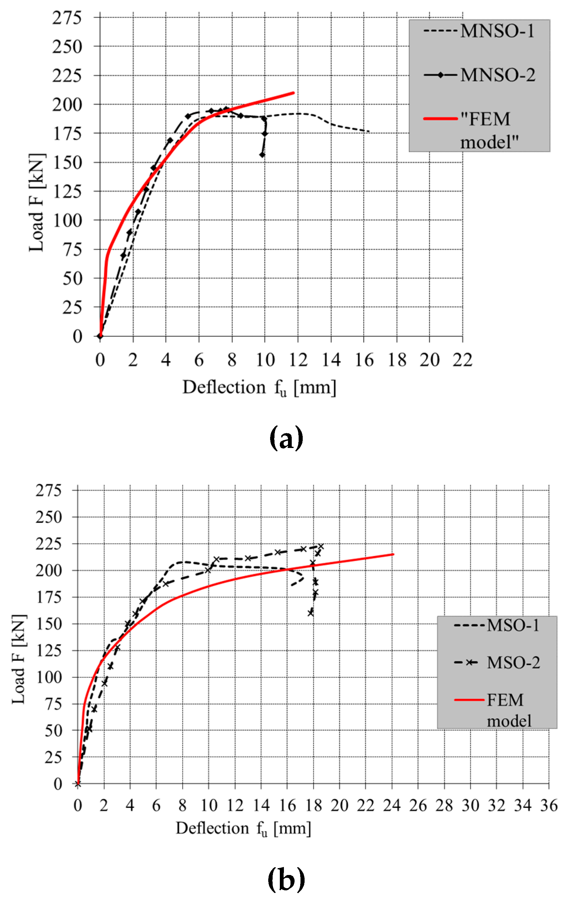
4.2. Full-Scale Walls

As for wall parts in the models of full-scale walls, the results of the numerical analysis were compatible with the experimental results regarding both the load-carrying capacity and the way they are damaged. The image of damaged parts of the walls obtained with the non-contact optical system during the laboratory tests and the numerical model at the failure phase are compared in Figure 20.

Results of the numerical analysis were compared with mean values of destructive force and deflection obtained for each series of the tested models. For the model MNSO, the maximum destructive force acting on the lintel was 210 kN, and the deflection was 11.7 mm. The obtained destructive force was greater by 9% than the force obtained during the tests, and the value of deflection constituted 36% of the experimentally obtained deflection. For the numerical model MSO, the obtained destructive force of 215 kN was equal to the test force, and the deflection of 24.1 mm was greater by 84% than the corresponding deflection obtained during the laboratory tests. Similar discrepancies between the results from the numerical analysis and laboratory tests were observed for the model M2SO. The destructive force of 255 kN was smaller by 4%, and the deflection of 23.4 mm was greater by 200% than the corresponding destructive force and deflection obtained during the laboratory tests. Figure 21 presents the relationship between the load and the displacement of the numerical models and the tests models of confined walls.

A few operating phases of the lintel/masonry/reinforced concrete elements could be distinguished in all tested models of walls. The elastic phase in the test and numerical models began from the moment of loading until the formation of the first cracks in the lintel induced by its deflection or a crack in the bed joint over the lintel (crack opening in the interface elements in the numerical model). Then, there was a post-elastic phase lasting from the moment of the lintel cracking (crack opening in the interface elements) to the moment of reaching the destructive force. After reaching the value of the ultimate force Fu, the model entered into the softening phase, during which a further increase in the lintel deflection occurred and was disproportional to the change in the loading force exerted on the research model. In that phase, cracks were significantly wider. Moreover, spalling of masonry units and loosening of the concrete cover were observed. The softening phase in the numerical model was not apparent, despite using the contact elements and the elastic–plastic model of the material. Further development of the applied model is required to include that phase in the numerical calculations. However, it is a difficult task, as the models behaved differently in the final phase after reaching the destructive force value. In the models with inner peripheral confinement (M2SO series), there was a rapid decrease in the load, whereas vertical displacements of the lintels were greater. In the non-confined MNOS models and the MSO models confined along their perimeter, the softening phase was mild. The destructive force obtained for non-confined walls was kept constant while deflection of the lintel was increasing. For the most confined walls (M2SO models), when the ultimate force was reached, there was an increase in deflection of the lintel and a simultaneous slight increase of the load.

The sequence of damage was similar in laboratory tests and numerical analyses. In the non-confined walls of the MNSO series, cracking was at first noticed in the lintel over supports at a deflection of ca. 0.8 mm obtained during the tests. Crack opening in the interface elements of the numerical model was observed later, at a deflection equal to 10 mm. In the next step, diagonal cracks were formed in the bottom part of the lintel, at the supports. In the final phase, numerous vertical cracks developed in the lintel supports.

The first cracks in the MSO models, confined along their perimeters, were induced by bending during displacement on the order of 0.5 mm. Later, loss of mortar adhesion to masonry units in the joint between the lintel and the masonry occurred. Crack opening in the interface elements occurred at a deflection equal to 0.7 mm. Furthermore, diagonal cracks developed and ran from the top edge of the lintel to the support, and then other diagonal cracks in the support zone were observed. The greatest cracks in the reinforced concrete spandrel beam were formed at the midspan of an opening, which was not surprising.

In the models with inner peripheral confinement (test and numerical M2SO models), the final arrangement of cracks was similar to the one in the models of the MSO series (the wall confined along the perimeter); however, the sequence of their formation was different. At first, the bed joint above the lintel was cracked at a displacement of 0.5 mm. Crack opening in the interface elements occurred at a deflection equal to 0.7 mm. Then, the cracks induced by bending developed at the midspan with simultaneous cracking at the junction with the reinforced concrete core. The post-elastic phase of the masonry/lintel/reinforced concrete layout was completed when the first diagonal cracks propagated from the bottom to the central area, and other cracks were running towards the support edge; however, they never reached the edge, unlike in the models of the MSO series. Failure of the tie beam occurred as a result of shearing. Analysing the course of crack development in lintels and reinforced concrete elements, as well as the results of the numerical analysis, it can be stated that the cores confining walls had an impact on the tie performance and the deformation level of walls.

As was observed in smaller models, there were some differences in deflections of the lintel obtained from the laboratory tests and the numerical model. The biggest difference was found for the unconfined model. Differences resulted from crack width in the laboratory models. Local crushing of the material was also observed in the real models, as opposed to the numerical model.

5. Conclusions

This paper described the procedure of modelling masonry constructions made of autoclaved aerated concrete. The strategy used for numerical modelling was presented. We proposed our own approach to homogenisation of the masonry units and the interface elements using the standard models. The applied material models, the structure of numerical models of wall parts and full-scale walls were discussed. The calculated results were shown using ATENA 2D software.

The conducted numerical analyses indicated that the comparison of the strength criterion and the elastic–plastic M-W-3 model, as well as the interface elements, can be used to track the morphology of cracks and the method of the model failure. The obtained results are satisfactory regarding the relationship of load-deflection at the elastic and hardening phases. The largest discrepancy between results from the calculations and the tests was found at the softening phase when the maximum load was reached. The method of plane modelling (2D) instead of real spatial conditions and the possible spread of material parameters for the masonry units and the wall in the post-failure phase had the greatest impact on the observed discrepancies. Further analyses will be performed on the modelling of walls using homogeneous models under spatial stress using 3D models.

References

1. Zienkiewicz, O.C.; Taylor, R.L. The Finite Element Method; MacGraw-Hill Book Company: New York, NY, USA, 1977. [Google Scholar]
2. Chen, W.F. Plasticity for Reinforced Concrete; McGraw-Hill Book Company: New York, NY, USA, 1982. [Google Scholar]
3. Jirásek, M.; Bazant, Z.P. Inelastic Analysis of Structures; John Wiley & Sons: Hoboken, NJ, USA, 2002. [Google Scholar]
4. Nasiri, E.; Liu, Y. Development of a detailed 3D FE model for analysis of the in-plane behaviour of masonry infilled concrete frames. Eng. Struct. 2017, 143, 603–616. [Google Scholar] [CrossRef]
5. Wendner, R.; Vorel, J.; Smith, J.; Hoover, C.G.; Bažant, Z.P.; Cusatis, G. Characterization of concrete failure behavior: A comprehensive experimental database for the calibration and validation of concrete models. Mater. A. Struct. 2015, 48, 3603–3626. [Google Scholar] [CrossRef]
6. Lemos, J.V. Discrete Element Modeling of the Seismic Behavior of Masonry Construction. Buildings 2019, 9, 43. [Google Scholar] [CrossRef] [Green Version]
7. Rasulo, A.; Pelle, A.; Lavorato, D.; Fiorentino, G.; Nuti, C.; Briseghella, B. Finite Element Analysis of Reinforced Concrete Bridge Piers Including a Flexure-Shear Interaction Model. Appl. Sci. 2020, 10, 2209. [Google Scholar] [CrossRef] [Green Version]
8. Drobiec, Ł. FEM model of the masonry made of hollow calcium silicate units. Proc. Eng. 2017, 193, 462–469. [Google Scholar] [CrossRef]
9. Drobiec, Ł. Limitation of cracking in AAC masonry under the window zone. Mauerwerk 2017, 21, 332–342. [Google Scholar] [CrossRef]
10. Drobiec, Ł. Analyse von Spannungen und Verformungen im Brüstungsbereich von Wandmodellen aus Porenbeton und Kalksandstein. Mauerwerk 2020, 24, 2–16. [Google Scholar] [CrossRef]
11. Marcon, M.; Vorel, J.; Ninšcević, K.; Wan-Wendner, R. Modeling Adhesive Anchors in a Discrete Element Framework. Materials 2017, 10, 917. [Google Scholar] [CrossRef] [Green Version]
12. Ceroni, F.; Darban, H.; Luciano, R. Analysis of bond behavior of injected anchors in masonry elements by means of Finite Element Modeling. Comp. Struct. 2020, 241, 112099. [Google Scholar] [CrossRef]
13. Christou, G.; Ungermann, J.; Wolters, K.; Hegger, J.; Claßen, M. Ermüdung von Verbunddübelleisten: Analyse und Modellentwicklung. Beton- und Stahlbetonbau. 2020, 115, 355–363. [Google Scholar] [CrossRef]
14. Deng, M.; Yang, S. Experimental and numerical evaluation of confined masonry walls retrofitted with engineered cementitious composites. Eng. Struct. 2020, 207, 110249. [Google Scholar] [CrossRef]
15. Nowak, R.; Orłowicz, R. Selected problems of failures and repairs of historic masonry vaults. MATEC Web Conf. 2019, 284, 05008. [Google Scholar] [CrossRef]
16. Abdellatef, M.; Alnaggar, M.; Boumakis, G.; Cusatis, G.; Di-Luzio, G.; Wendner, R. Lattice Discrete Particle Modeling for coupled concrete creep and shrinkage using Solidification Microprestress Theory. CONCREEP 2015, 10, 184–193. [Google Scholar]
17. Rita, M.; Fairbairn, E.; Ribeiro, F.; Andrade, H.; Barbosa, H. Optimization of Mass Concrete Construction Using a Twofold Parallel Genetic Algorithm. Appl. Sci. 2018, 8, 399. [Google Scholar] [CrossRef] [Green Version]
18. Ponikiewski, T.; Steidl, T.; Krause, P. Moisture transport in cellular concrete walls with the connector for thermal insulation. Period. Polytech. Civ. Eng. 2018, 62, 986–991. [Google Scholar] [CrossRef] [Green Version]
19. Drobiec, Ł.; Wyczółkowski, R.; Kisiołek, A. Numerical Modelling of Thermal Insulation of Reinforced Concrete Ceilings with Complex Cross-Sections. Appl. Sci. 2020, 10, 2642. [Google Scholar] [CrossRef] [Green Version]
20. Podroužek, J.; Marcon, M.; Ninšcević, K.; Wan-Wendner, R. Bio-Inspired 3D Infill Patterns for Additive Manufacturing and Structural Applications. Materials. 2019, 12, 499. [Google Scholar] [CrossRef] [Green Version]
21. Drobiec, Ł. FEM Micro-Model for Masonry Reinforced in Bed Joints. Proc. Brit. Mason. Soc. 2006, 5, 2005. [Google Scholar]
22. Jasiński, R. Numerical Analysis of the Strains and Stress States Reinforced Clay Brick Masonry Walls Horizontally Sheared. Int. J. Eng. Technol. Manag. 2018, 8, 20–37. [Google Scholar] [CrossRef]
23. Drobiec, Ł.; Jasiński, R. Adoption of the Willam-Warnke failure criterion for describing behavior of Ca-Si hollow blocks. Procedia Engin. 2017, 193, 470–477. [Google Scholar] [CrossRef]
24. Jasiński, R. Identification of the Parameters of Menetrey -Willam Failure Surface of Calcium Silicate Units. IOP Conference Series. Mat. Sci. Eng. 2017, 245, 032045. [Google Scholar] [CrossRef]
25. D’Altri, A.M.; Messali, F.; Rots, J.; Castellazzi, G.; De Miranda, S. A damaging block-based model for the analysis of the cyclic behaviour of full-scale masonry structures. Eng. Fr. Mech. 2019, 209, 423–448. [Google Scholar] [CrossRef]
26. D’Altri, A.M.; Sarhosis, V.; Milani, G.; Rots, J.; Cattari, S.; Lagomarsino, S.; Sacco, E.; Tralli, A.; Castellazzi, G.; de Miranda, S. Modeling Strategies for the Computational Analysis of Unreinforced Masonry Structures: Review and Classification. Arch. Comput. Methods Eng. 2019, 1–33. [Google Scholar] [CrossRef]
27. Mazur, W.; Drobiec, L.; Jasiński, R. Research of Light Concrete Precast Lintels. Proc. Engin. 2016, 161, 611–617. [Google Scholar] [CrossRef] [Green Version]
28. Mazur, W.; Drobiec, Ł.; Jasiński, R. Research and numerical investigation of masonry—AAC precast lintels interaction. Procedia Eng. 2017, 193, 385–392. [Google Scholar] [CrossRef]
29. Drobiec, Ł.; Jasiński, R.; Mazur, W. Precast lintels made of autoclaved aerated concrete—Test and theoretical analyses. Cement Wapno Beton 2017, 5, 339–413. [Google Scholar]
30. Chu, T.C.; Ranson, W.F.; Sutton, M.A.; Peters, W.H. Application of digital-image-correlation techniques to experimental mechanics. Experiment. Mech. 1985, 25, 232–244. [Google Scholar] [CrossRef]
31. Lourenço, P.B. Computational Strategies for Masonry Structures. Ph.D. Thesis, Delft University, Delft, The Netherland, 1996. [Google Scholar]
32. Lourenço, P.B.; Rots, J.G.; Blaauwendraad, J. Two Approaches for the Analysis of Masonry Structures. Micro Macro-Modeling. Heron. 1995, 4, 313–340. [Google Scholar]
33. Gambrotta, L.; Logomarsino, S. Damage models for the seismic response of trick masonry shear walls. Part I. The mortar joint model and its applications. Earthq. Eng. Struct. Dynam. 1997, 26, 423–439. [Google Scholar] [CrossRef]
34. Gambrotta, L.; Logomarsino, S. Damage models for the seismic response of trick masonry shear walls. Part II. The continuum model and its applications. Earthq. Eng. Struct. Dynam. 1997, 26, 441–462. [Google Scholar] [CrossRef]
35. Lopez, J.; Oller, S.; Onnte, E.; Lubliner, J. A Homogeneous Constitutive Model for Masonry. Int. J. Num. Meth. Eng. 1999, 46, 149–156. [Google Scholar] [CrossRef]
36. Lourenço, P.B.; Rots, J.G.; Blaauwendraad, J. Continuum Model for Masonry: Parameter Estimation and Validation. ASCE J. Struct. Eng. 1998, 124, 642–652. [Google Scholar] [CrossRef]
37. Lourenço, P.B. On the Use of Homogenization Techniques for the Analysis of Masonry Structures. Mason. Int. 1997, 1, 26–32. [Google Scholar]
38. Lourenço, P.B. Two Aspect Related to the Analysis of Masonry Structures: Size Effect and Parameter Sensibility; Technische Universiteit Delft: Delft, The Netherland, 1997. [Google Scholar]
39. Lotfi, H.R.; Shing, P.B. Interface Model Applied to Fracture of Masonry Structures. ASCE J. Struct. Eng. 1994, 1, 63–80. [Google Scholar] [CrossRef]
40. Jasiński, R. Research and Modelling of Masonry Shear Walls. Ph.D. Thesis, Silesian University of Technology, Gliwice, Poland, 2017. [Google Scholar]
41. Alfaiate, J.; de Almeida, J.R. Modelling Discrete Cracking on Masonry Walls. Masonry International. J. Brit. Mason. Soc. 2004, 2, 83–93. [Google Scholar]
42. Jasiński, R. Validation of elastic-brittle, and elastic-plastic FEM model of the wall made of calcium silicate and AAC masonry units. IOP Conference Series. Mat. Sci. Eng. 2019, 603, 1757–8981. [Google Scholar] [CrossRef] [Green Version]
43. Červenka, J.; Papanikolaou, V.K. Three dimensional combined fracture-plastic material model for concrete. Int. J. Plasticity. 2008, 24, 2192–2220. [Google Scholar] [CrossRef]
44. Hordijk, D.A. ocal Approach to Fatigue of Concrete. Ph.D. Thesis, Delft University, Delft, The Netherland, 1991. [Google Scholar]
45. Code, M. Fib Model Code for Concrete Structures; Ernst & Sohn: Berlin, Germany, 2010. [Google Scholar]
46. Kupfer, H.; Hilsdorf, H.K.; Rüsch, H. Behavior of Concrete under Biaxial Stress. J. Am. Concr. Inst. Proc. 1969, 8, 656–666. [Google Scholar]
47. Menétrey, P.; Willam, K.J. Triaxial failure criterion for concrete and its generalization. Aci Struct. J. 1995, 92, 311–318. [Google Scholar] [CrossRef]
48. Hoek, E.; Brown, E.T. Empirical Criterion for Rock Masses. J. Geotech. Eng. Div. 1980, 106, 1575. [Google Scholar]
49. Weihe, S. Implicit Integration Schemes for Multi-Surface Yeld Criteria Subjected to Hardening/Softening Behavior. Master’s Thesis, University of Colorado-Boulder, Boulder, Colorado, 1989. [Google Scholar]
50. Červenka, V.; Červenka, J. ATENA Program Documentation. Copyright 2000–2015 Červenka Consulting s.r.o. Prague, 2015. Available online: https://www.cervenka.cz/assets/files/atena-pdf/ATENA-Engineering-2D_Tutorial.pdf (accessed on 6 August 2020).
51. Červenka, V. Constitutive model for cracked reinforced concrete. J. Proc. 1985, 82, 877–882. [Google Scholar] [CrossRef]
52. Bruehwiler, E.; Wittman, F.H. The Wedge Splitting Test, A New Method of Performing Stable Fracture-Mechanics Tests. Eng. Fract. Mech. 1990, 35, 117–125. [Google Scholar] [CrossRef]
53. Drobiec, Ł.; Jasiński, R.; Rybarczyk, T. The influence of the type of mortar on the compressive behaviour of walls made of Autoclaved Aerated Concrete (AAC). In Brick and Block Masonry—Trends, Innovations and Challenges; Taylor & Francis Group: London, UK, 2016; pp. 1531–1538. [Google Scholar]
54. Jasiński, R. Research on the Influence of Bed Joint Reinforcement on Strength and Deformability of Masonry Shear Walls. Materials 2019, 12, 2543. [Google Scholar] [CrossRef] [PubMed] [Green Version]
55. Drobiec, Ł. Analysis of AAC walls subjected to vertical load. Mauerwerk 2019, 23, 387–403. [Google Scholar] [CrossRef]
Figure 1. Adopting various strategies for developing the micro-model of the wall with thin-layer joints with unfilled head joints on the basis of [32,33,34,41,42]: (a) real structure of modelled masonry, (b) spatial micro-model of the wall (3D-F), (c) two-dimensional micro-model of the wall (2D-C), (d) two-dimensional micro-model of the wall (2D-D), (e) two-dimensional micro-model of the wall (2D-CD), (f) two-dimensional micro-model of the wall (2D-M) with masonry units having the equivalent non-linear parameters of the masonry; 1—masonry unit, 2—mortar in bed joints, 3—masonry unit of linear or non-linear parameters, 5—mortar in bed joints of linear or non-linear parameter, 6—masonry unit of linear or non-linear parameters, 7—mortar in bed joints of linear or non-linear parameters, 8—masonry unit of linear parameters, 9—contact element of bed joints of non-linear parameters, 10—contact element of bed joints of non-linear parameters, 11—masonry unit of non-linear parameters, 12—masonry unit of equivalent non-linear parameters of the wall.
Applsci 10 05446 g001
Figure 2. Equivalent uniaxial stress-strain relationship for elastic model with material degradation.
Applsci 10 05446 g002
Figure 3. Exponential relationship determining crack width of the SBeta model.
Applsci 10 05446 g003
Figure 4. Compressive stress–strain relationship.
Applsci 10 05446 g004
Figure 5. Failure criterion for material under biaxial stress state on the basis of [46].
Applsci 10 05446 g005
Figure 6. Elliptical curve shape 0.5 r ( Θ , e ) 1.0 .
Applsci 10 05446 g006
Figure 7. Menétrey–Willam criterion in Haigh–Westergaard space: (a) the space of principal stresses, (b) hydrostatic cross-section, (c) deviatoric section.
Applsci 10 05446 g007
Figure 8. The Rankine criterion in Haigh–Westergaard space: (a) the space of principal stresses, (b) axiatoric section, (c) deviatoric section.
Applsci 10 05446 g008
Figure 9. The relative position of the Rankine and M-W-3 surfaces at λt = 2: (a) view of surfaces in principal stress space, (b) axiatoric sections, (c) deviatoric sections; 1—Rankine surface, 2—M-W-3 surface at k = 1 (yield strength), 3—M-W-3 surface at k = ko (end of elastic stage).
Applsci 10 05446 g009
Figure 10. Shape of hardening/softening function [43].
Applsci 10 05446 g010
Figure 11. Failure criterion taken for contact elements: 1—boundary surface, 2—residual surface.
Applsci 10 05446 g011
Figure 12. The relationship of shear stress and normal stress with displacement of contact elements (a) at shearing, (b) under tension; 1—default function of softening.
Applsci 10 05446 g012
Figure 13. Simplified softening laws (a) for normal tensile stresses, (b) for cohesion (initial shearing strength).
Applsci 10 05446 g013
Figure 14. The Huber–Mises–Hencky yield surface: (a) the space of principal stresses, (b) axiatoric section, (c) deviatoric section.
Applsci 10 05446 g014
Figure 15. The Prandtl-Reuss model: (a) bilinear relationship σ-ε, (b) law of kinematic hardening: 1—initial location of yield surface, 2—subsequent location of yield surface.
Applsci 10 05446 g015
Figure 16. Numerical models of wall parts used in finite element method (FEM) calculations for the following series: (a) model of elements of the numeral model I (NI) series, (b) model of elements of the NII series, (c) model of elements of the NIII series: 1—masonry units with the elastic-plastic based M-W-3 model, 2—reinforced concrete elements with the brittle model, 3—contact elements in bed joints, 4—contact elements in head joints, 5—finite elements representing reinforcement with the Huber–Mises–Hencky (H-M-H) model.
Applsci 10 05446 g016
Figure 17. Numerical models of walls used in FEM calculations for the following series: (a) model of MNSO wall, (b) model of MSO wall, (c) model of M2SO wall: 1—masonry units with the elastic-plastic based M-W-3 model, 2—reinforced concrete elements with the elastic-brittle based model, 3—contact elements in bed joints, 4—contact elements in head joints, 5—finite elements representing reinforcement with the H-M-H model.
Applsci 10 05446 g017
Figure 18. Damage recorded by the optical system compared with the damage to the numerical model for the elements of the following series: (a) NI, (b) NII, (c) NIII.
Applsci 10 05446 g018
Figure 19. Compared relationship between the load and deflection of the lintel determined experimentally and from numerical calculations for the models of the following series: (a) NI, (b) NII, (c) NIII.
Applsci 10 05446 g019aApplsci 10 05446 g019b
Figure 20. Comparison of damage recorded by the optical system and the deformation in the numerical model of the walls of series: (a) MNSO, (b) MSO, (c) M2SO.
Applsci 10 05446 g020
Figure 21. Compared relationship between the load and the displacement of the lintel, determined experimentally and from numerical calculations for the models of the following series: (a) MNSO, (b) MSO, (c) M2SO.
Applsci 10 05446 g021aApplsci 10 05446 g021b