Using Committee Neural Network for Prediction of Pressure Drop in Two-Phase Microchannels

Abstract

Numerous studies have proposed to correlate experimental results, however there are still significant errors in those predictions. In this study, an artificial neural network (ANN) is considered for a two-phase flow pressure drop in microchannels incorporating four neural network structures: multilayer perceptron (MLP), radial basis function (RBF), general regression (GR), and cascade feedforward (CF). The pressure drop predication by ANN uses six inputs (hydraulic diameter of channel, critical temperature of fluid, critical pressure of fluid, acentric factor of fluid, mass flux, and quality of vapor). According to the experimental data, for each network an optimal number of neurons in the hidden layer is considered in the range 10–11. A committee neural network (CNN) is fabricated through the genetic algorithm to improve the accuracy of the predictions. Ultimately, the genetic algorithm designates a weight to each ANN model, which represents the relative contribution of each ANN in the pressure drop predicting process for a two-phase flow within a microchannel. The assessment based on the statistical indexes reveals that the results are not similar for all models; the absolute average relative deviation percent for MLP, CF, GR, and CNN were obtained to be equal to 10.89, 10.65, 7.63, and 5.79, respectively. The CNN approach is demonstrated to be superior to many ANN techniques, even with simple linearity in the model.

1. Introduction

During recent years, much research has been conducted on two-phase inside microchannels to survey transport phenomena. There are many examples for the process involving two-phase flow in microchannels: microreactors, miniature heat exchangers, fuel injection in internal combustion equipment, miniature refrigeration systems, cooling of high-powered electronic systems, fusion reactors for cooling plasma-facing components, and fuel cells with evaporator components [1,2,3,4].

Nevertheless, two-phase flows inside microchannels come with disadvantages, too. They impose a higher pressure drop through the fluid flow passing through narrow channels. Hence, both pressure drop and heat transfer considerations should simultaneously be taken into account during the design process of these miniaturized heat exchangers.

Numerous experimental datasets have been collected and studied by scholars, to investigate inside two-phase flow microchannels [5,6,7,8]. For instance, there are published experimental works that explore fluid characteristics inside microchannels with a two-phase flow of nitrogen, R12, R32, R134a, R236ea, R245fa, R404a, R410a, and R422 with different qualities and mass fluxes at different channel hydraulic diameters [9,10,11].

Harirchian and Garimella [12] considered a boiling of the dielectric liquid fluorinert FC-77 in parallel microchannels to investigate heat transfer coefficients and pressure. They studied the flow and boiling phenomena for a comprehensive range of channels in four distinct flow regimes, including slug, annular, bubbly, and alternating churn/annular/wispy-annular flow regimes.

Pan et al. [13] experimentally examined the characteristics of flow boiling of deionized water inside a microchannel consisting of 14 parallel channels with 0.15 × 0.25 mm rectangular shape. They selected the heat flux, mass flux, and inlet temperature as significant factors for the variation of pressure drop. Based on the experiment results, they concluded from the pressure drop trend that with the increasing quality of vapor, instability will be increased.

Meanwhile, researchers have tried to validate the adiabatic pressure drop correlations of two-phase flow inside microchannels for different conditions by comparing them with the comprehensive databases at hand. Some researchers [14,15,16,17,18] have studied the heat transfer coefficient for flow boiling of oxygen-free streams inside copper microchannel heat sinks. The experimental results are in good agreement with the corresponding numerical predictions. Maher et al. [19] proposed a set of new equations to describe a two-phase pressure drop, along with the homogeneous flow of different working fluids at different tube diameters and fluid flux values.

Although many correlations are provided by researchers for predicting pressure drops, having a comprehensive correlation for an extensive range of factors for linear multivariate modeling is too difficult. A common way to obtain a comprehensive correlation is to use non-linear empirical modeling techniques, such as artificial neural network (ANN), which is developed based on the brain’s biological neuron network function [20,21,22,23].

The artificial neural network method has been increasingly used to solve engineering problems. Using an appropriate form of the algorithm to train and test the network configurations would be followed by the successful application of ANN. Picanco et al. [24] suggested that the functional relations between the pertinent dimensionless numbers in nucleate boiling can be correlated to convective heat transfer through a genetic algorithm. The flow pattern of two-phase water and air stream was presented by Mehta et al. [25]. They found predictor correlations by means of applying the ANN method on a circular Y-junction minichannel with a 2.1 mm diameter.

According to the literature, there has been limited effort focused on evaluating the pressure drop by means of the ANN technique. Therefore, in this study, in addition to the use of conventional neural networks in engineering sciences to achieve higher levels of accuracy, we have integrated these models using the concept of committee neural network. As such, different neural network models were employed, and then a committee neural network was generated, based on a genetic algorithm to integrate the neural networks.

2. Methods

2.1. Artificial Neural Networks

Artificial Neural Network (ANN) is a system of data processing, describing, predicting, and clustering which is inspired by the biological nervous system [26]. The nerve cell is the smallest component of this system. The data gained from experiments, or the measurements, are inputs of this system. The relative importance of the inputs is assigned by weights, and the weighted input values are combined by the summing function. Evaluation of information takes place by processing the obtained data from the summing function and the outputs of the activation unit. The nature of the relationship between artificial neural cells and biological neurons is illustrated in Figure 1. As shown in this figure, a similar manner of processing collected data from the outside world exists for both an artificial neural cell and a biological neuron.

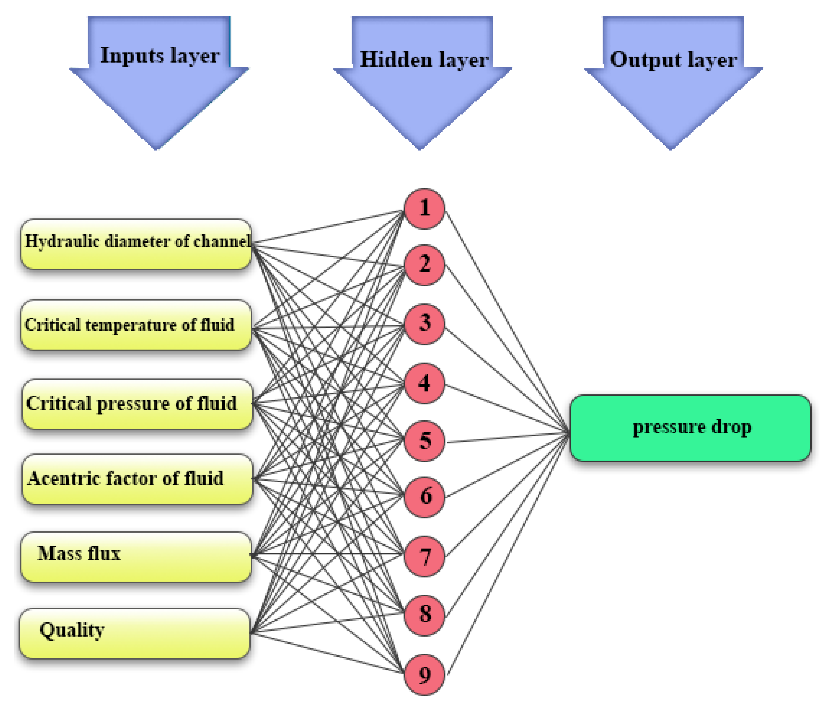
For this purpose, the input layer takes variables from resources like experimental data to do some mathematical operations. Then these values are sent to the hidden layers, in which the number of hidden layers can be specified regarding the complexity of problems. The estimation of output value for all ANN structures can be provided as below:

$$Y_{i. pred}=f\left({\displaystyle \sum }_{i=1}^n{w}_i{x}_i+b\right)$$

(1)

where the output value ($Y_{i. pred}$) is computed using a function f and the summation of the multiplication of weight $w_i$ and input $x_i$ to the bias b.

In general, ANN models predict the output parameters according to the following procedure:

• Training trends are determined based on datasets.
• The architecture of the neural network is defined.
• The network parameters are determined.
• The feedforward back-propagation program is run.
• Data are compared and analyzed.

In this study, the pressure drop, as the output, is essentially the target, and is predicted by compiling the testing inputs data. Inputs 1 to 6 are hydraulic diameter of channel, critical temperature of fluid, critical pressure of fluid, acentric factor of fluid (a concept referring to the molecule’s shape), mass flux, and quality (the mass fraction of vapor in a saturated mixture), respectively.

Table 1. Range of the input parameters.

Variable	Name	Minimum Value	Maximum Value
Hydraulic diameter of channel (mm)	Input 1	0.078	3
Critical temperature of fluid (K)	Input 2	345	419
Critical pressure of fluid (MPa)	Input 3	3.73	11.3
Acentric factor of fluid (-)	Input 4	0.152	0.37
Mass flux (kg·m−2·s−1)	Input 5	196.9	1400
Quality (%)	Input 6	0.007	0.961

presents the values of these input parameters.

Various models of the artificial neural network can be utilized in the prediction and comparison of experimental data results. Classification of these networks is dependent on their application. In this paper, four specific types of neural networks, such as multilayer perceptron, radial basis function, cascade feedforward, and general regression, are employed for estimations.

2.1.1. Multilayer Perceptron (MLP)

Multilayer perceptron (MLP) was developed in 1986, and it has become the most commonly used type of artificial neural network to solve problems by estimation [27]. These networks have a number of layers between their input and output layers, and their learning algorithm is essentially based on a gradient descent technique, which is basically a back-propagation algorithm. The back-propagation networks aim to approximate the network outputs according to the desired output, with the aim of reducing error. Ultimately, error reduction is achieved by setting the network weight values in the subsequent iteration.

2.1.2. Radial Basis Function (RBF)

Broomhead and Lowe developed a type of feedforward neural network named the radial basis function neural network [28]. The main difference between MLP and RBF methodologies is that the RBF method includes hidden layers containing radial basis activation functions.

2.1.3. Cascade Feedforward (CF)

Feedforward and cascade forward networks make use of the back-propagation algorithm regardless of the connection between neurons in each layer. In cascade forward networks, neurons are connected to both the neurons in the previous layers, as well as all the neurons in the same layer [29]. Similar to feedforward back-propagation networks, the back-propagation algorithm is also used by cascade networks for updating weights. The main feature of a cascade neural network is that in each layer, neurons are associated with all neurons in the previous layer.

2.1.4. General Regression (GR)

The general regression neural network is used for estimation of a continuous variable, similar to the standard regression technique. However, GR is superior with regards to fast learning and converging into optimal regression [30]. GR is structured by four layers: input, pattern, output, and summation layers. GR might be recognized as a fully connected network, since its layers are linked to the following layer through weighting vectors between neurons. This method is used to determine the nonlinear relationship between variables.

2.1.5. Committee Neural Network (CNN)

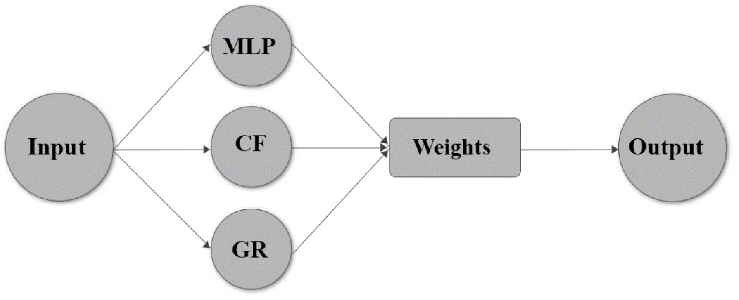
In general, a set of neural networks is making up the committee neural network, and it offers the benefits of the whole work by integrating the product of individual systems. Therefore, a model can act better than the finest individual network. CNN is used as an optimization method to reach the final result through a combination of the outputs of different models [31,32]. Figure 2 shows a schematic representation of a committee neural network. A combiner integrates the models in various ways; the most common way is the simple averaging of the group. Meanwhile, the genetic algorithm (GA) can help properly combine the weight (contribution) of each neural network in CNN. This approximation method incorporates the principles of genetics and natural selection. Therefore, a set of networks makes up CNN, and it incorporates the benefits of the whole work by means of integrating the product of each individual mode.

2.2. Experimental Database

In this study, the databank obtained from different experimental studies [33,34,35,36,37,38] was used for the investigation of pressure drop. Available experimental results in the literature demonstrate that the pressure drop in microchannels is influenced by the vapor quality and other fluid properties. Therefore, as reported in

Table 2. Range and conditions of various experimental datasets.

Hydraulic Diameter of Channel (mm)	Critical Temperature of Fluid (K)	Critical Pressure of Fluid (MPa)	Acentric Factor of Fluid (-)	Mass Flux (kg·m−2· s−1)	Quality (%)	Pressure Drop (kPa· m−1)	Ref
1.4	345–419	3.78–4.9	0.296–0.37	196.8–1394.4	0.26–0.79	15.8–145	[33]
0.078–2.1	345–406	4.07–11.3	0.152–0.33	290–450	0.007–0.96	81.4–3814.7	[34]
2.13–6.2	345.2–374	3.73–4.99	0.215–0.33	400–1000	0.08–0.86	5.33–34.8	[35]
2.64	385	4.14	0.179	400–1400	0.11–0.9	4.36–56.5	[36]
0.24–0.79	374	4.07	0.33	270–950	0.08–0.95	34.1–2318.18	[37]
3	352.65	3.9	0.284	198–350	0.19–0.93	9.72–82.4	[38]

, a total of 329 empirical data points was selected for modeling, and various neural networks were examined for data training purposes. The collected experimental data covers the quality ranging from 0.007 to 0.96, mass flux of 196.8–1400 kg·m⁻²·s⁻¹, acentric factor from 0.152 to 0.33, critical pressure of 3.73–11.3 MPa, critical temperature of 345–419 K, and hydraulic diameter values ranging from 0.078 to 6.2.

2.3. Scaling Database and Transformation

The provision for employing the ANN method is that there should not be any units when training begins. The reason is that the limit for the neuron output to be in the range [0, 1] is imposed by non-linear activation functions, such as a hyperbolic or logistical tangent. The standardization of data for ANN computations was done by the statistical normalization rule. After calculation completion, the output data from the network were reverse converted to their original representation. To improve the efficiency of the training step in the ANN calculations, Equation (2) was used to normalize the inputs and target values.

$$V_{normal}=0.01+\frac{V-V_{min}}{V_{max}-V_{min}}\times \left(0.99-0.01\right)$$

(2)

In this equation, V signifies the variables, whether they be dependent or independent, and V_normal represents the normal value. The maximum and minimum values of each variable are shown by V_max and V_min, respectively.

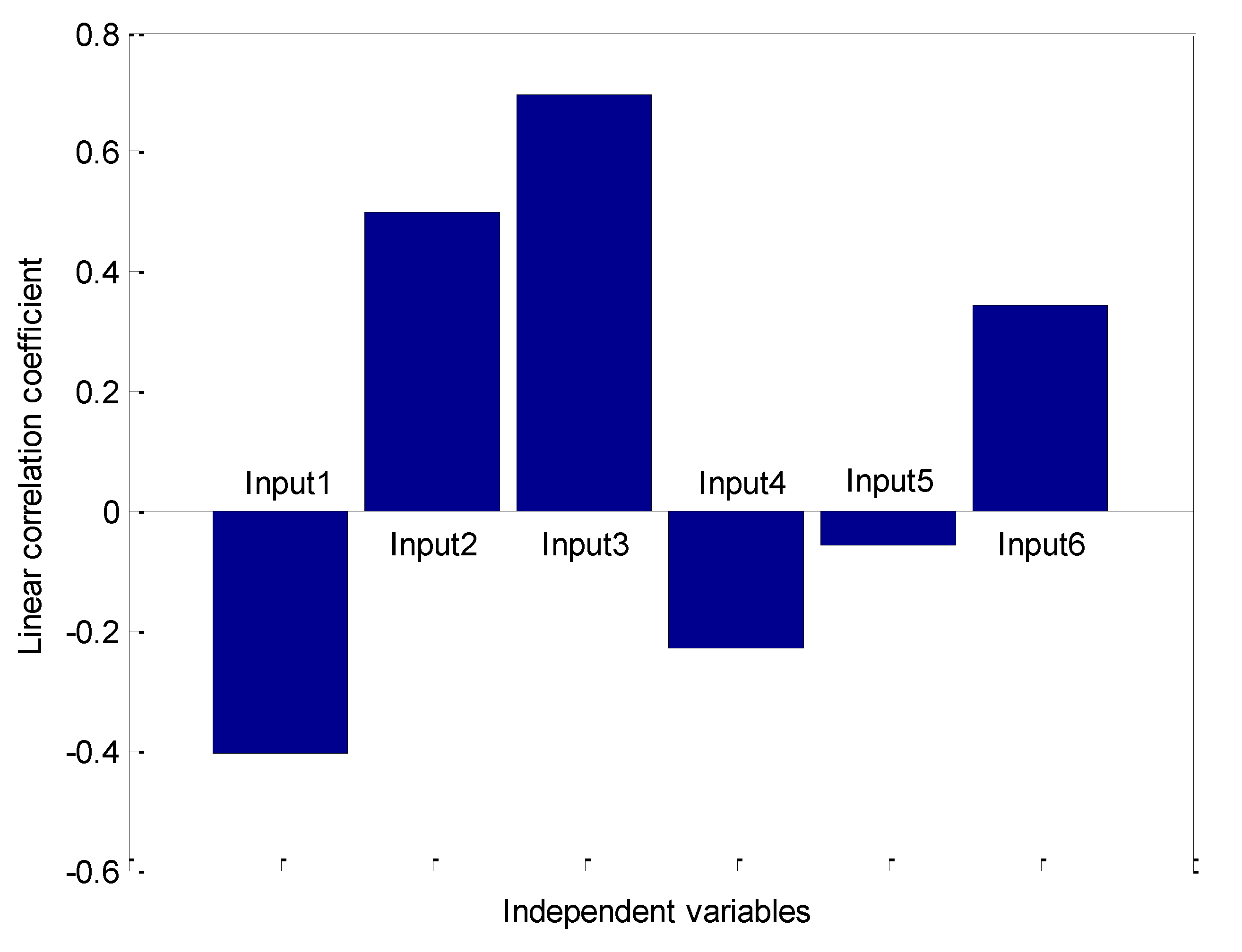
The process of selecting suitable inputs for ANN is accomplished by means of the Pearson correlation coefficient, which is a measure for variable rating. The connection type and intensity between sets of variables are determined by the Pearson correlation coefficient. This coefficient takes the values in a range between −1 and +1, which respectively correspond to the highest reverse and direct association cases. This coefficient is equal to 0 if there is no association between variables. The most important variables are the absolute averaged ones, since they have an imperative close interaction. Thus, the relationship between independent and dependent variables would be most credible when the maximization of average absolute Pearson’s coefficient (AAPC) is performed for a particular dependent variable transformation. The Pearson correlation coefficient values between each pair of variables are represented in Figure 3.

It is evident from this figure that the most influential direct and indirect relationships belong to critical temperature of fluid and hydraulic diameter of the channel, respectively. This is while mass flux has the least linearity with pressure drop in the microchannel.

Table 3. Pearson’s coefficient values for different transformations.

Transformation		Pearson’s Coefficient						AAPC
Function	Number	Input1	Input2	Input3	Input4	Input5	Input6
1	Output 15	−0.0901	0.1866	0.2583	−0.0386	−0.0197	0.1399	0.1222
2	Output 14	−0.0937	0.1941	0.2687	−0.0402	−0.0205	0.1451	0.127
3	Output 13	−0.0977	0.2026	0.2805	−0.0419	−0.0214	0.151	0.1325
4	Output 12	−0.1022	0.2122	0.2938	−0.0439	−0.0223	0.1575	0.1387
5	Output 11	−0.1072	0.2232	0.3089	−0.0461	−0.0234	0.1649	0.1456
6	Output 10	−0.1128	0.2356	0.3261	−0.0486	−0.0245	0.1732	0.1535
7	Output 2	−0.2513	0.4708	0.6433	−0.1434	−0.0379	0.3129	0.3099
8	Output	−0.4043	0.501	0.697	−0.2293	−0.0594	0.3419	0.3721
9	Output 0.75	−0.4757	0.4917	0.6936	−0.2519	−0.0744	0.3372	0.3874
10	Output 0.5	−0.5610	0.4676	0.6727	−0.2643	−0.0949	0.3196	0.3967
11	Output 0.25	−0.6489	0.4254	0.6274	−0.2559	−0.1188	0.2855	0.3937
12	Output 0.1	−0.6941	0.3919	0.5875	−0.2377	−0.1322	0.2584	0.3836
13	Output −0.1	0.7349	−0.3412	−0.5226	0.1987	0.1454	−0.2189	0.3603
14	Output −0.25	0.7465	−0.3021	−0.4693	0.1618	0.15	−0.1909	0.3368
15	Output −0.5	0.7298	−0.2422	−0.3824	0.097	0.1469	−0.1545	0.2921
16	Output −0.75	0.6811	−0.1939	−0.3082	0.0407	0.1336	−0.1338	0.2486
17	Output −1	0.6193	−0.1578	−0.2508	−0.0009	0.1162	−0.1255	0.2117
18	Output −2	0.4213	−0.0843	−0.1384	−0.0663	0.0642	−0.1297	0.1507
19	Output −10	0.1041	0.0198	−0.0360	−0.0800	0.0278	−0.0967	0.0607
20	Output −11	0.0965	0.0221	−0.0338	−0.0797	0.0275	−0.0939	0.0589
21	Output −12	0.0908	0.0239	−0.0322	−0.0795	0.0273	−0.0917	0.0575
22	Output −13	0.0865	0.0254	−0.0310	−0.0793	0.0272	−0.0899	0.0565
23	Output −14	0.0833	0.0265	−0.0300	−0.0792	0.0271	−0.0886	0.0558
24	Output −15	0.0809	0.0274	−0.0293	−0.0791	0.0271	−0.0876	0.0552
25	exp(Output)	-	-	-	-	-	-	-
26	Log(Output)	−0.7178	0.3671	0.5563	−0.2200	−0.1397	0.2387	0.3733

contains the inputs and different transformations. This figure indicates that the best possible outcome for pressure drop is obtained from the output to the power of 0.5. Eventually, the transformation should be reversed to reach the modeling dependent variables and enable its comparison with the actual values.

3. Results and Discussion

3.1. Performance Analysis of Models

To compare the precision of the model, various statistical indexes, such as absolute average relative deviation percent (AARD%), mean square error (MSE), the regression coefficient (R²), and root mean square error (RMSE), have been utilized. These indexes are introduced as follows:

$$AARD\%=\frac{1}{N}{\displaystyle \sum }_{i=1}^N(\left|\frac{Y_{i.real}-Y_{i.pred}}{Y_{i.real}}\right|)\times 100$$

(3)

$$MSE=\frac{1}{N}{\displaystyle \sum }_{i=1}^N{\left(Y_{i.real}-Y_{i.pred}\right)}^2$$

(4)

$$R^2=\frac{{{\displaystyle \sum }}_{i=1}^N{\left(Y_{i.real}-{\overline{Y}}_{real}\right)}^2-{{\displaystyle \sum }}_{i=1}^N{\left(Y_{i.real}-Y_{i.pred}\right)}^2}{{{\displaystyle \sum }}_{i=1}^N{\left(Y_{i.real}-{\overline{Y}}_{raal}\right)}^2}$$

(5)

$$RMSE=\sqrt{\frac{1}{N}{\displaystyle \sum }_{i=1}^N{\left(Y_{i.real}-Y_{i.pred}\right)}^2}$$

(6)

where $Y_{i. real}$, ${\overline{Y}}_{act}$, and $Y_{i. pred}$ represent the real values, the mean of real values, and values of predicted pressure drop, respectively. Moreover, N indicates the dataset’s number.

3.2. Selecting the Configuration of ANNs

According to the literature, the dataset was divided into testing and training portions, comprising 15% and 85% of the entire experimental dataset, respectively; this is done to confirm the consistency of expected models. Determination of weights and topology of a network is called the optimization process, and results in the optimum function when specific performance equations are utilized. The determination of the number of optimal neurons contained in the hidden layer is of great importance. The number of inputs, outputs, the architecture of the network, and the algorithm used for training can all affect the optimum number of neurons in a hidden layer. As expressed by Ayoub and Demiral [39], determining the optimum number of hidden neurons is not simple, and cannot be performed without training, and solely by examining different numbers of them to estimate each generalization error. Bar and Das [40] demonstrated that a single hidden layer having enough number of processing units would have an acceptable performance. As such, we chose a single hidden layer with multiple processing neurons in this study.

The trial and error method was used to develop a successful model. The dominant statistical parameters, such as the average absolute relative error, correlation coefficient, and root mean squared errors, were examined for all of the topologies. This provided the opportunity for careful inspection and visualization of the cross-validation or generalization error of each network design.

As mentioned before, the optimization of the MLP was done by changing the neuron content of the hidden layer while the statistical indexes were monitored. The minimum number of data needed for training is 2–11 times of weight and bias. Hence, for an MLP that has one dependent and six independent variables, the number of hidden neurons were computed as follows:

$$\begin{gathered} 3\times \left(8N+1\right)\le 279\left(training\right) \\ N\le 11 \end{gathered}$$

(7)

The best outcomes of the MLP network for the number of hidden neurons are presented in

Table 4. Determining the greatest hidden neurons for multilayer perceptron (MLP).

Hidden Neuron	Dataset	Statistical Index
		AARD%	MSE	RMSE	R2
1	Train	101.57	113,482.04	336.871	0.9004
	Test	129.45	140,778.92	375.205	0.9111
	Total	104.36	116,220.03	340.911	0.9017
2	Train	53.22	55,622.25	235.844	0.9502
	Test	68.21	279,407.52	528.59	0.8965
	Total	54.73	78,068.80	279.408	0.9362
3	Train	37.34	57,662.92	240.131	0.9519
	Test	53.07	70,940.72	266.347	0.9407
	Total	38.92	58,994.74	242.888	0.9507
4	Train	34.92	52,085.74	228.223	0.96
	Test	28.75	28,003.70	167.343	0.9048
	Total	34.3	49,670.22	222.868	0.9588
5	Train	27.89	49,789.84	223.136	0.957
	Test	25.89	60,526.28	246.021	0.9626
	Total	27.69	50,866.74	225.537	0.9576
6	Train	25	44,457.30	210.849	0.9624
	Test	32.34	66,664.92	258.195	0.9532
	Total	25.73	46,684.82	216.067	0.9612
7	Train	17.86	7611.552	87.244	0.9941
	Test	39.8	23,686.50	153.904	0.9832
	Total	20.06	9223.933	96.041	0.9929
8	Train	16.82	5794.544	76.122	0.995
	Test	23.06	16,642.14	129.004	0.9919
	Total	17.45	6882.601	82.961	0.9946
9	Train	12.7	3905.889	62.497	0.997
	Test	27.03	7658.826	87.515	0.9892
	Total	14.13	4282.324	65.439	0.9965
10	Train	12.1	3631.65	60.263	0.9972
	Test	16.12	8260.039	90.885	0.9893
	Total	12.5	4095.895	63.999	0.9966
11	Train	10.33	5773.065	75.981	0.9956
	Test	15.91	3095.685	55.639	0.9974
	Total	10.89	5504.513	74.192	0.9957

.

Considering the minimum MSE value and the maximum R-squared value, eleven hidden neurons in MLP networks are optimum. The efficiencies of different types of ANNs were compared to find a suitable model for pressure drop prediction. Hence, a comparison was performed between the optimum MLP network structure and other ANN models, such as CF, RBF, and GR. The exactness of sensitivity for finding the optimum hidden neurons number is listed in

Table 5. Performance of cascade feedforward (CF) model with different hidden neurons.

Hidden Neuron	Dataset	Statistical Index
		AARD%	MSE	RMSE	R2
1	Train	41.35	77,007.54	277.502	0.9338
	Test	43.68	72,265.35	268.822	0.9546
	Total	41.59	76,531.88	276.644	0.936
2	Train	36.82	57,041.61	238.834	0.949
	Test	31.08	106,981.54	327.08	0.9572
	Total	36.24	62,050.78	249.1	0.9482
3	Train	33.54	49,877.14	223.332	0.9573
	Test	48.86	87,864.31	296.419	0.941
	Total	35.08	53,687.40	231.705	0.9553
4	Train	27.2	52,898.02	229.996	0.9572
	Test	41.79	31,827.33	178.402	0.9651
	Total	28.66	50,784.55	225.354	0.9577
5	Train	23.85	33,742.42	183.691	0.9721
	Test	23.06	54,227.72	232.868	0.9552
	Total	23.77	35,797.18	189.201	0.9704
6	Train	19.92	10,395.52	101.958	0.9913
	Test	33.18	25,249.53	158.901	0.9845
	Total	21.25	11,885.43	109.02	0.9904
7	Train	13.88	5371.999	73.294	0.9961
	Test	20.71	5675.702	75.337	0.9934
	Total	14.57	5402.462	73.501	0.9957
8	Train	12.99	5365.915	73.252	0.9958
	Test	22.3	4866.778	69.762	0.9946
	Total	13.92	5315.849	72.91	0.9957
9	Train	11.48	5250.163	72.458	0.9958
	Test	23.74	10,279.86	101.39	0.9911
	Total	12.71	5754.662	75.859	0.9953
10	Train	9.78	2434.457	49.34	0.998
	Test	18.48	7820.685	88.435	0.9926
	Total	10.65	2974.717	54.541	0.9976

,

Table 6. Performance of radial basis function (RBF) model with different hidden neurons.

Hidden Neuron	Spread	Dataset	Statistical Index
			AARD%	MSE	RMSE	R2
1	2.1212	Train	245.61	168,040.37	409.927
		Test	113.14	235,995.95	485.794	0.8892
		Total	232.32	174,856.58	418.159	0.8624
2	1.0101	Train	127.73	132,611.39	364.158	0.8856
		Test	131.98	150,529.48	387.981	0.8964
		Total	128.15	134,408.64	366.618	0.8862
3	0.7071	Train	98.76	101,348.30	318.352	0.9176
		Test	141.53	94,193.30	306.909	0.8996
		Total	103.05	100,630.63	317.223	0.9151
4	0.8081	Train	79.53	95,710.78	309.372	0.9196
		Test	140.55	103,820.68	322.212	0.9242
		Total	85.65	96,524.24	310.684	0.919
5	0.6061	Train	84.45	73,306.36	270.751	0.9367
		Test	69.94	100,134.85	316.441	0.939
		Total	83	75,997.36	275.676	0.9368
6	0.6061	Train	84.04	73,687.32	271.454	0.9413
		Test	66.43	49,203.87	221.819	0.9572
		Total	82.28	71,231.53	266.892	0.9404
7	0.6061	Train	78.14	68,354.82	261.448	0.9443
		Test	58.43	83,310.02	288.635	0.9363
		Total	76.17	69,854.89	264.301	0.9419
8	0.6061	Train	71.69	63,860.08	252.706	0.9466
		Test	55.92	79,202.58	281.43	0.9464
		Total	70.11	65,398.99	255.732	0.9461
9	0.6061	Train	67.33	56,511.36	237.721	0.9546
		Test	73.26	122,784.88	350.407	0.921
		Total	67.92	63,158.85	251.314	0.9471
10	0.7071	Train	63.84	65,435.85	255.804	0.9468
		Test	78.67	88,688.61	297.806	0.9383
		Total	65.33	67,768.20	260.323	0.9431
11	0.7071	Train	57.93	57,530.63	239.855	0.9467
		Test	70.16	143,614.80	378.965	0.9632
		Total	59.16	66,165.21	257.226	0.9469

and

Table 7. Accuracy of the general regression (GR) for prediction.

Spread	Dataset	Statistical Index
		AARD%	MSE	RMSE	R2
0.0056	Train	2.42	2688.514	51.851	0.9979
	Test	34.47	129,915.53	360.438	0.9381
	Total	7.63	15,449.89	124.298	0.9881

. It should be noted that the determination of the number of hidden neurons is similar in all kinds of ANNs and has regulations similar to MLP.

The hidden neurons were not significant in the GR, therefore the spread value needed to be modified to reach the significant hidden neurons in GR. Accordingly, one hundred statistical indicators of various GRs were compared with regards to the spread value changes within 0.1–10, with 0.1 interval steps.

Table 8. Comparison of the statistical values for various artificial neural network (ANN) models.

Model	Dataset	Statistical Index
		AARD%	MSE	RMSE	R2
MLP	Train	10.33	5773.065	75.981	0.9956
	Test	15.91	3095.685	55.639	0.9974
	Total	10.89	5504.513	74.192	0.9957
CF	Train	9.78	2434.457	49.34	0.998
	Test	18.48	7820.685	88.435	0.9926
	Total	10.65	2974.717	54.541	0.9976
GR	Train	2.42	2688.514	51.851	0.9979
	Test	34.47	129,915.53	360.438	0.9381
	Total	7.63	15,449.89	124.298	0.9881
RBF	Train	57.93	57,530.63	239.855	0.9467
	Test	70.16	143,614.80	378.965	0.9632
	Total	59.16	66,165.21	257.226	0.9469

lists the values of AARD%, MSE, RMSE, and R² obtained from different ANN models with the best topology.

Rationally, the AARD% values of the best models are minimum. As indicated in Table 8, the best prediction of the pressure drop belongs to the GR model, compared to other models. By considering the values obtained as the statistical error of pressure drop, the AARD% of the GR model (with the error value of 7.63) yielded the best prediction, compared with other ANN models of MLP (10.89), RBF (59.16), and CF (10.65).

It should be noted that the statistical indices of R², MSE, RMSE, and AARD% served as the basis for choosing this model amongst a set of 1620 distinct models (1100 RBF models, 200 CF models, 100 GR models, 220 MLP models).

3.3. Comparison of CNN with Other Neural Networks

As mentioned before, the CNN method is made up of two steps for predicting pressure drop parameters. The first is by applying it in committee neural network methodology to determine pressure drop parameters, and the second one is implementing it in a genetic algorithm to find the share (weight) of each algorithm in building CNN.

By joining the outputs of the three models MLP, GR, and CF, the microchannel pressure drop was predicted in more precision. It should be noted that, due to the high error of the RBF method, the predicted data from this model has not been used in the CNN model. To describe the coefficient of every single model, GA is merged as follows:

$$Y_{CNN}=\left(a{Y}_{MLP}+b{Y}_{GR}+c{Y}_{CF}+d\right)$$

(8)

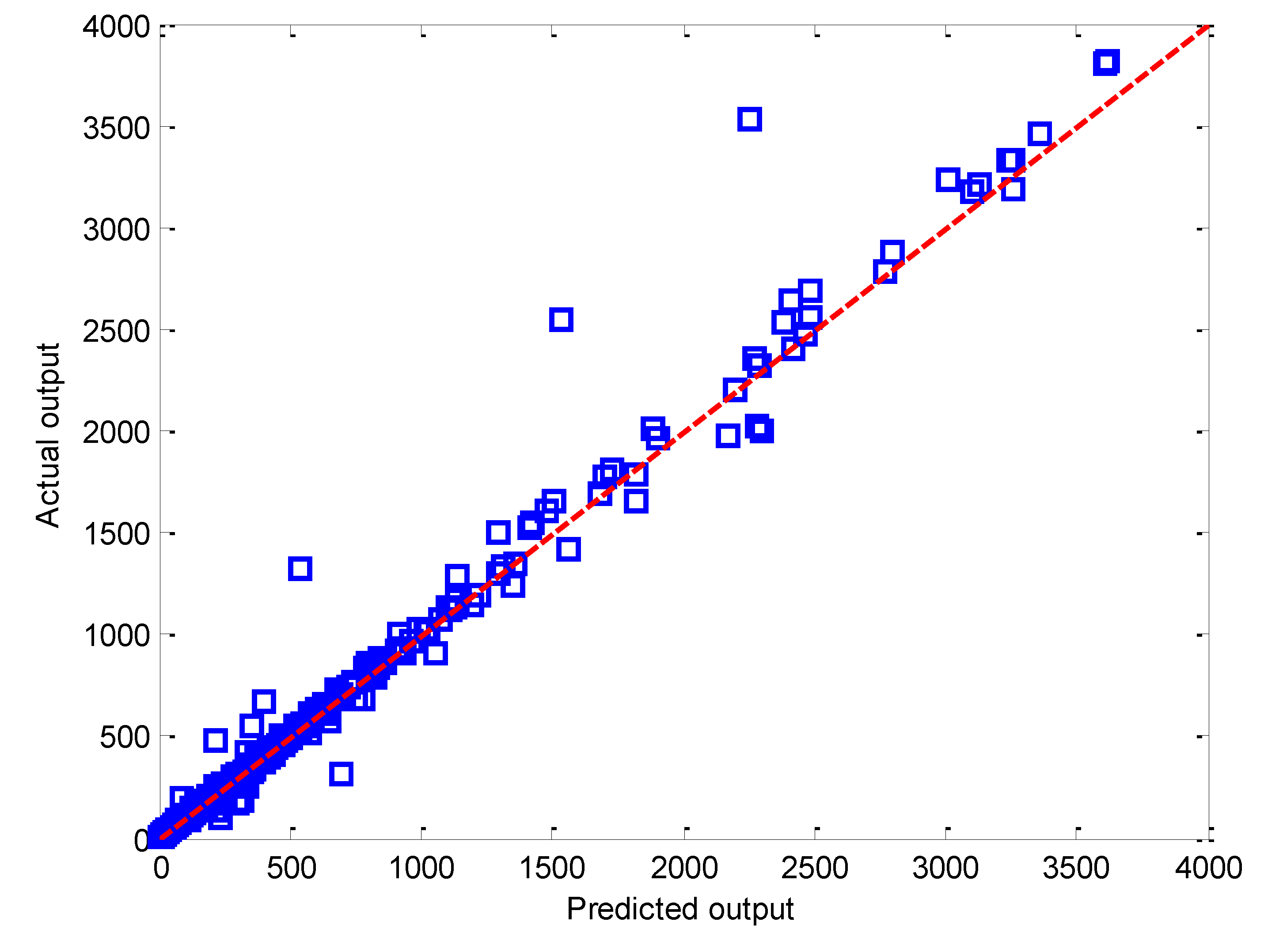
where calculated values of $a$, $b$, $c$ and $d$ are 0.0534, 0.9281, 0.01725, and −0.1574, respectively. Figure 4 illustrates the actual outputs versus the values of predicted outputs by CNN for the entire dataset of pressure drop. It is evident that the CNN model is remarkably capable of forecasting results for the whole dataset, as the concentration of symbols around the solid 45° line confirms this.

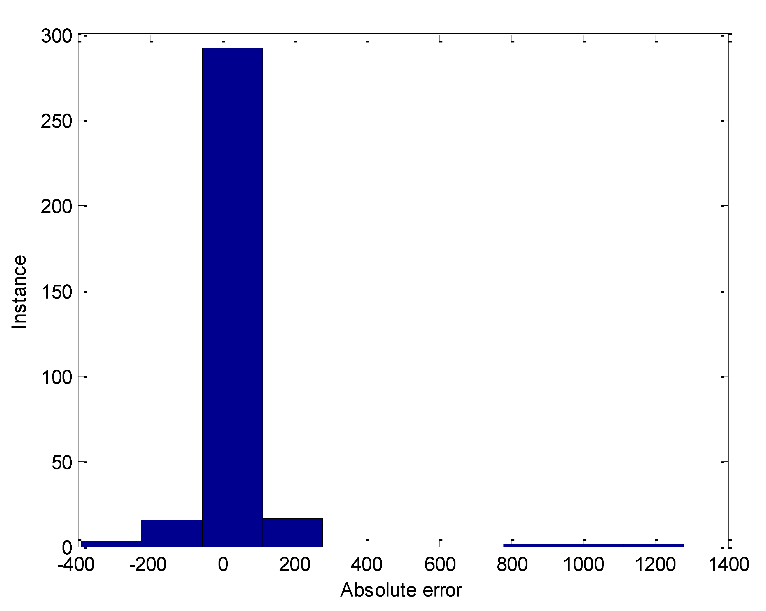
The absolute error histogram for the entire data by the CNN network is presented in Figure 5, which is an approximately normal distribution. As shown, it can be seen that the absolute error distribution histogram is stable, and most of the prediction errors belong to the −200 to 200 absolute error intervals.

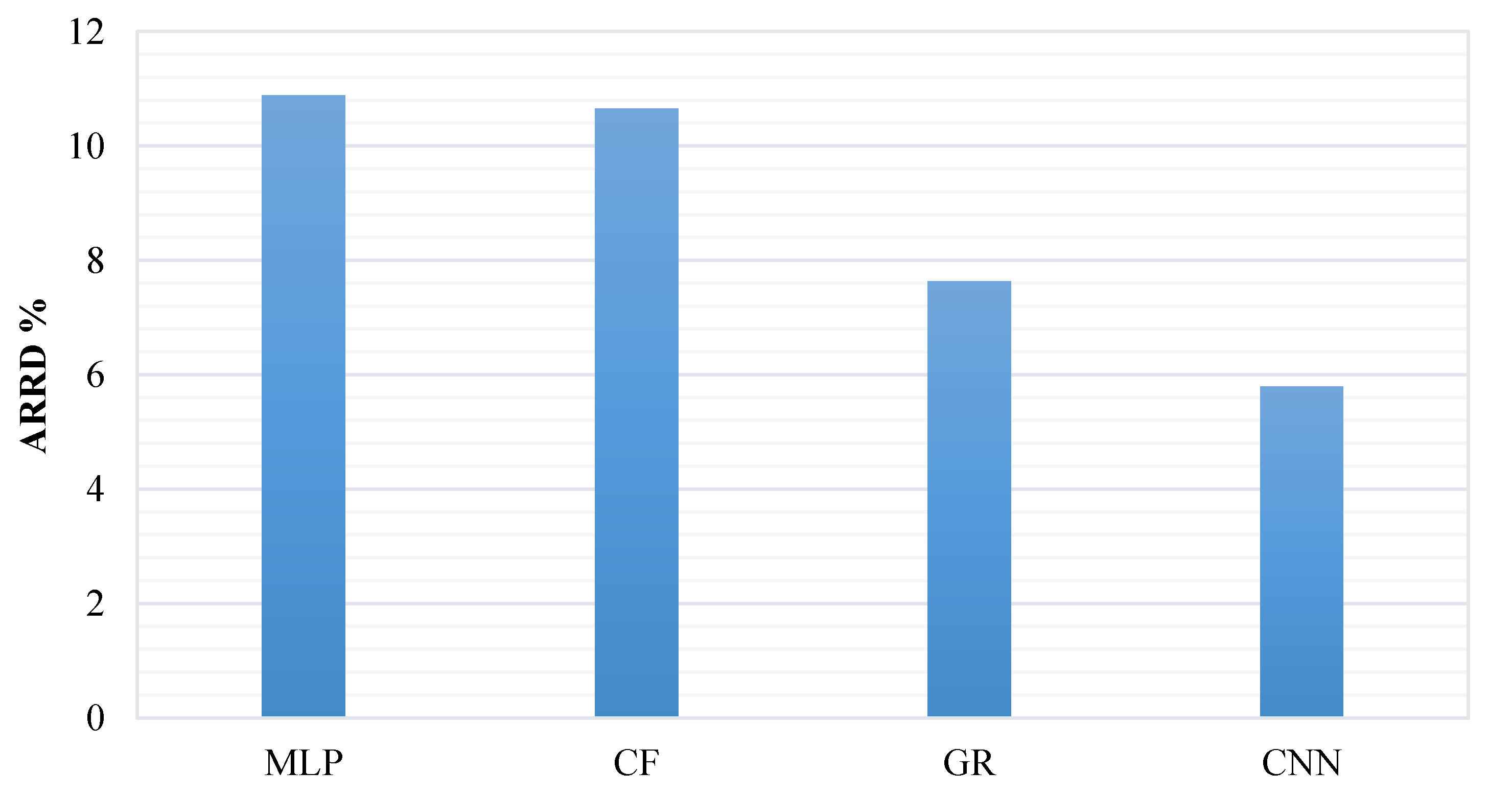
The comparison between the suggested CNN model and the three other models of MLP, CF, and GR are presented in Figure 6, based on the statistical indices of AARD%. This figure indicates the performance superiority of the CNN model, compared with the other models. In other words, it depicts the capability of CNN to increase the accuracy of the prediction.

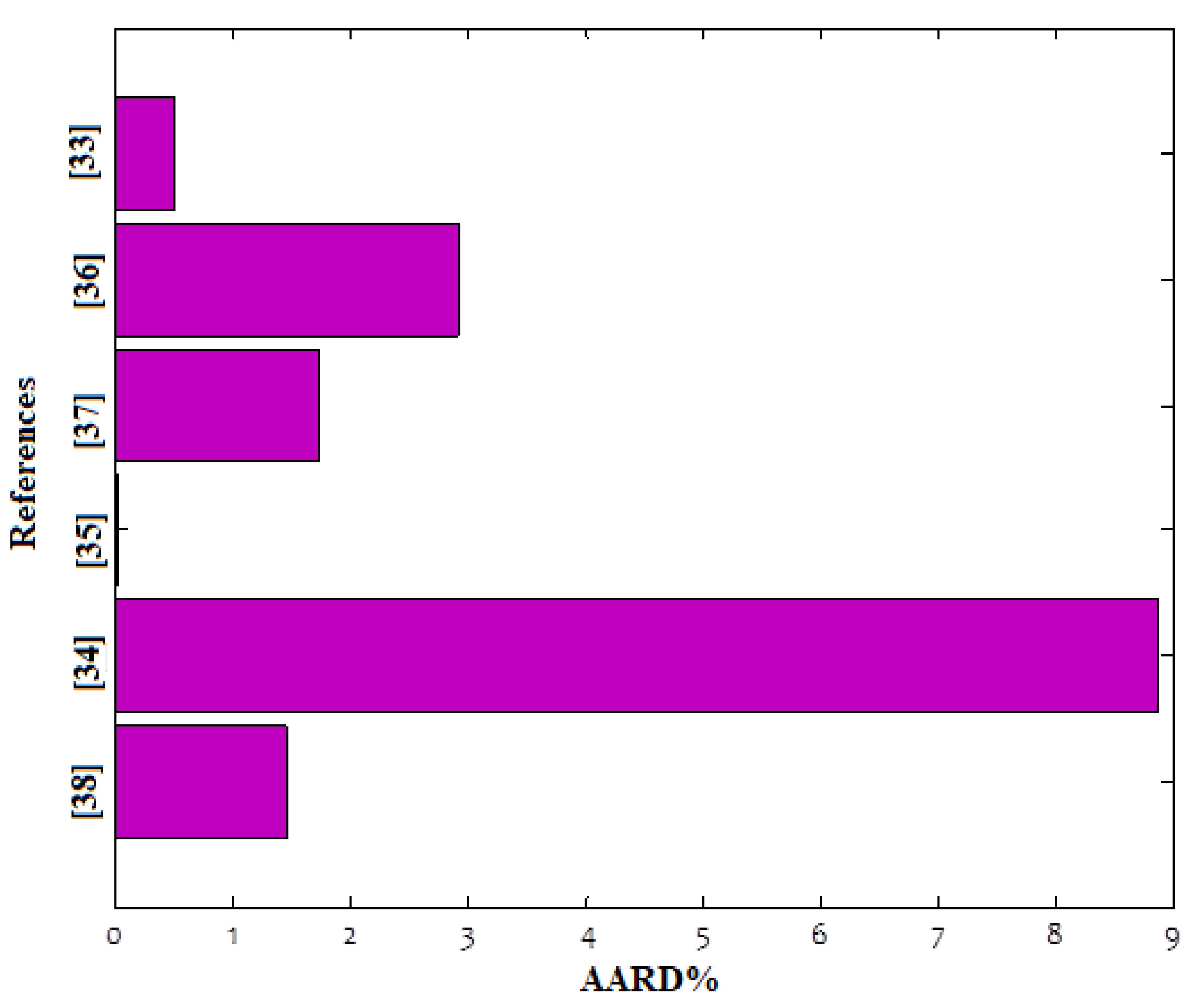
Finally, the predicted values from the CNN model representing microchannel pressure drop prediction were evaluated for different experimental datasets. The AARD% values in Figure 7 were obtained to compare the predicted values and experimental datasets. As can be seen, the CNN model can predict all experimental data with great accuracy. However, the predictive precision of the CNN model can slightly depend on the distribution pattern of the data, as expected. This is consistent with the recent data of [41].

4. Conclusions

In this study, the pressure drop was predicted using a committee neural network (CNN). As such, a total number of 329 empirical data points were selected to model the pressure drop in microchannels at various conditions. The results reveal that despite the low dependency of the pressure drop on the mass flux, it is highly dependent on the properties of the fluid. Nevertheless, the plot of the pressure drop as a function of variables revealed its dependency on the hydraulic diameter of the channel and vapor quality. The weight coefficient of each network in CNN was determined using a genetic algorithm and a simple averaging method. The minimum AARD% is achieved when using a simple averaging procedure for combining MLP, GR, and CF algorithms. The finest value of AARD% (5.79) is obtained by combining all algorithms using the weighted averaging method. The values of 0.0534, 0.9281, and 0.01725 were obtained as the derived weights of GA for MLP, GR, and CF, respectively. This study demonstrates that CNN results are more precise when there are various techniques to solve a problem, therefore the superior results, compared to the other methods, indicate a high potential for prediction in different fields of applied science.

References

1. Almasi, F.; Shadloo, M.S.; Hadjadj, A.; Ozbulut, M.; Tofighi, N.; Yildiz, M. Numerical simulations of multi-phase electro-hydrodynamics flows using a simple incompressible smoothed particle hydrodynamics method. Comput. Math. Appl. 2019. [Google Scholar] [CrossRef]
2. Sadeghi, R.; Shadloo, M.S.; Hopp-Hirschler, M.; Hadjadj, A.; Nieken, U. Three-dimensional lattice Boltzmann simulations of high density ratio two-phase flows in porous media. Comput. Math. Appl. 2018, 75, 2445–2465. [Google Scholar] [CrossRef]
3. Giannetti, N.; Redo, M.A.; Jeong, J.; Yamaguchi, S.; Saito, K.; Kim, H. Prediction of two-phase flow distribution in microchannel heat exchangers using artificial neural network. Int. J. Refrig. 2020, 111, 53–62. [Google Scholar] [CrossRef]
4. Mahvi, A.J.; Garimella, S. Two-phase flow distribution of saturated refrigerants in microchannel heat exchanger headers. Int. J. Refrig. 2019, 104, 84–94. [Google Scholar] [CrossRef]
5. Chachereau, Y.; Chanson, H. Free-Surface Turbulent Fluctuations and Air-Water Flow Measurements in Hydraulics Jumps with Small Inflow Froude Numbers; The University of Queensland: Queensland, Australia, 2010. [Google Scholar]
6. Chen, X.; Hou, Y.; Chen, S.; Liu, X.; Zhong, X. Characteristics of frictional pressure drop of two-phase nitrogen flow in horizontal smooth mini channels in diabatic/adiabatic conditions. Appl. Therm. Eng. 2019, 162, 114312. [Google Scholar] [CrossRef]
7. Bahmanpouri, F. Experimental Study of Air Entrainment in Hydraulic Jump on Pebbled Rough Bed. Ph.D. Thesis, The University of Napoli Federico II, Naples, Italy, 2019. [Google Scholar]
8. Lillo, G.; Mastrullo, R.; Mauro, A.W.; Pelella, F.; Viscito, L. Experimental thermal and hydraulic characterization of R448A and comparison with R404A during flow boiling. Appl. Therm. Eng. 2019, 161, 114146. [Google Scholar] [CrossRef]
9. Filho, E.d.S.; Aguiar, G.M.; Ribatski, G. Flow boiling heat transfer of R134a in a 500 µm ID tube. J. Braz. Soc. Mech. Sci. Eng. 2020, 42, 254. [Google Scholar] [CrossRef]
10. Lewis, J.M.; Wang, Y. Two-phase frictional pressure drop in a thin mixed-wettability microchannel. Int. J. Heat Mass Transf. 2019, 128, 649–667. [Google Scholar] [CrossRef]
11. Vozhakov, I.S.; Ronshin, F.V. Experimental and theoretical study of two-phase flow in wide microchannels. Int. J. Heat Mass Transf. 2019, 136, 312–323. [Google Scholar] [CrossRef]
12. Harirchian, T.; Garimella, S.V. Flow regime-based modeling of heat transfer and pressure drop in microchannel flow boiling. Int. J. Heat Mass Transf. 2012, 55, 1246–1260. [Google Scholar] [CrossRef] [Green Version]
13. Pan, L.; Yan, R.; Huang, H.; He, H.; Li, P. Experimental study on the flow boiling pressure drop characteristics in parallel multiple microchannels. Int. J. Heat Mass Transf. 2018, 116, 642–654. [Google Scholar] [CrossRef]
14. Lee, J.; Mudawar, I. Two-phase flow in high-heat-flux micro-channel heat sink for refrigeration cooling applications: Part II—heat transfer characteristics. Int. J. Heat Mass Transf. 2005, 48, 941–955. [Google Scholar] [CrossRef]
15. Qu, W.; Mudawar, I. Flow boiling heat transfer in two-phase micro-channel heat sinks––I. Experimental investigation and assessment of correlation methods. Int. J. Heat Mass Transf. 2003, 46, 2755–2771. [Google Scholar] [CrossRef]
16. Lee, S.; Mudawar, I. Investigation of flow boiling in large micro-channel heat exchangers in a refrigeration loop for space applications. Int. J. Heat Mass Transf. 2016, 97, 110–129. [Google Scholar] [CrossRef]
17. Ramesh, B.; Jayaramu, P.; Gedupudi, S. Subcooled flow boiling of water in a copper microchannel: Experimental investigation and assessment of predictive methods. Int. Commun. Heat Mass Transf. 2019, 103, 24–30. [Google Scholar] [CrossRef]
18. Raj, S.; Pathak, M.; Khan, M.K. Effects of flow loop components in suppressing flow boiling instabilities in microchannel heat sinks. Int. J. Heat Mass Transf. 2019, 141, 1238–1251. [Google Scholar] [CrossRef]
19. Maher, D.; Hana, A.; Habib, S. New Correlations for Two Phase Flow Pressure Drop in Homogeneous Flows Model. Therm. Eng. 2020, 67, 92–105. [Google Scholar] [CrossRef]
20. Moayedi, H.; Aghel, B.; Vaferi, B.; Foong, L.K.; Bui, D.T. The feasibility of Levenberg–Marquardt algorithm combined with imperialist competitive computational method predicting drag reduction in crude oil pipelines. J. Pet. Sci. Eng. 2020, 185, 106634. [Google Scholar] [CrossRef]
21. Davoudi, E.; Vaferi, B. Applying artificial neural networks for systematic estimation of degree of fouling in heat exchangers. Chem. Eng. Res. Des. 2018, 130, 138–153. [Google Scholar] [CrossRef]
22. Aghel, B.; Rezaei, A.; Mohadesi, M. Modeling and prediction of water quality parameters using a hybrid particle swarm optimization–neural fuzzy approach. Int. J. Environ. Sci. Technol. 2018, 16, 4823–4832. [Google Scholar] [CrossRef]
23. Moayedi, H.; Aghel, B.; Foong, L.K.; Bui, D.T. Feature validity during machine learning paradigms for predicting biodiesel purity. Fuel 2020, 262, 116498. [Google Scholar] [CrossRef]
24. Picanço, M.A.S.; Passos, J.C.; Filho, E.P.B. Heat Transfer Coefficient Correlation for Convective Boiling Inside Plain and Microfin Tubes Using Genetic Algorithms. Heat Transf. Eng. 2009, 30, 316–323. [Google Scholar] [CrossRef]
25. Mehta, H.B.; Pujara, M.P.; Banerjee, J. Prediction of two phase flow pattern using artificial neural network. Network 2013, 5, 6. [Google Scholar]
26. Da Silva, I.N.; Spatti, D.H.; Flauzino, R.A.; Liboni, L.; Alves, S.F.D.R. Artificial Neural Network Architectures and Training Processes. In Artificial Neural Networks; Springer: Cham, Switzerland, 2017; pp. 21–28. [Google Scholar]
27. Liu, W.; Shadloo, M.S.; Tlili, I.; Maleki, A.; Bach, Q.-V. The effect of alcohol–gasoline fuel blends on the engines’ performances and emissions. Fuel 2020, 276, 117977. [Google Scholar] [CrossRef]
28. Broomhead, D.S.; Lowe, D. Radial Basis Functions, Multi-Variable Functional Interpolation and Adaptive Networks; Royal Signals and Radar Establishment Malvern: Malvern, Worcestershire, UK, 1988. [Google Scholar]
29. Zheng, Y.; Shadloo, M.S.; Nasiri, H.; Maleki, A.; Karimipour, A.; Tlili, I. Prediction of viscosity of biodiesel blends using various artificial model and comparison with empirical correlations. Renew. Energy 2020, 153, 1296–1306. [Google Scholar] [CrossRef]
30. Zhao, C.; Wu, G.; Li, Y. Measurement of water content of oil-water two-phase flows using dual-frequency microwave method in combination with deep neural network. Meas 2019, 131, 92–99. [Google Scholar] [CrossRef]
31. Bagheripour, P. Committee neural network model for rock permeability prediction. J. Appl. Geophys. 2014, 104, 142–148. [Google Scholar] [CrossRef]
32. Barzegar, R.; Moghaddam, A.A. Combining the advantages of neural networks using the concept of committee machine in the groundwater salinity prediction. Model. Earth Syst. Environ. 2016, 2, 26. [Google Scholar] [CrossRef] [Green Version]
33. Rosato, A.; Mauro, A.W.; Mastrullo, R.; Vanoli, G.P. Experiments during flow boiling of a R22 drop-in: R422D adiabatic pressure gradients. Energy Convers. Manag. 2009, 50, 2613–2621. [Google Scholar] [CrossRef] [Green Version]
34. Field, B.S.; Hrnjak, P. Adiabatic Two-Phase Pressure Drop of Refrigerants in Small Channels. In Proceedings of the ASME 4th International Conference on Nanochannels, Microchannels, and Minichannels, Parts A and B, Limerick, Ireland, 19–21 June 2006; Volume 2006, pp. 1173–1180. [Google Scholar]
35. Zhang, M.; Webb, R.L. Correlation of two-phase friction for refrigerants in small-diameter tubes. Exp. Therm. Fluid Sci. 2001, 25, 131–139. [Google Scholar] [CrossRef]
36. Hwang, Y.W.; Kim, M.S. The pressure drop in microtubes and the correlation development. Int. J. Heat Mass Transf. 2006, 49, 1804–1812. [Google Scholar] [CrossRef]
37. Yang, C.-Y.; Webb, R.L. Friction pressure drop of R-12 in small hydraulic diameter extruded aluminum tubes with and without micro-fins. Int. J. Heat Mass Transf. 1996, 39, 801–809. [Google Scholar] [CrossRef]
38. Cavallini, A.; Del Col, D.; Doretti, L.; Matkovič, M.; Rossetto, L.; Zilio, C. Two-phase frictional pressure gradient of R236ea, R134a and R410A inside multi-port mini-channels. Exp. Therm. Fluid Sci. 2005, 29, 861–870. [Google Scholar] [CrossRef]
39. Ayoub, M.A.; Demiral, B.M. Application of resilient back-propagation neural networks for generating a universal pressure drop model in pipelines. Univ. Khartoum Eng. J. 2011, 1, 9–21. [Google Scholar]
40. Bar, N.; Das, S.K. Gas-non-Newtonian Liquid Flow Through Horizontal Pipe–Gas Holdup and Pressure Drop Prediction using Multilayer Perceptron. Am. J. Fluid Dyn. 2012, 2, 7–16. [Google Scholar] [CrossRef] [Green Version]
41. Shadloo, M.S.; Rahmat, A.; Karimipour, A.; Wongwises, S. Estimation of pressure drop of two-phase fluid in horizontal long pipes using artificial neural networks. J. Energy Resour. Technol. 2020, 1–21. [Google Scholar] [CrossRef]
Figure 1. Schematic structure of the artificial neural network for estimating pressure drop.
Applsci 10 05384 g001
Figure 2. Structure of the committee neural network.
Applsci 10 05384 g002
Figure 3. Pearson correlation coefficients between each pair of independent variables.
Applsci 10 05384 g003
Figure 4. Performance of the committee neural network (CNN) for prediction.
Applsci 10 05384 g004
Figure 5. Histogram of CNN for all data.
Applsci 10 05384 g005
Figure 6. Evaluation between predicted values of three artificial neural network models and committee neural network.
Applsci 10 05384 g006
Figure 7. Evaluation of predicted values with regards to various experimental datasets in the literature.
Applsci 10 05384 g007