Susceptibility to Seismic Amplification and Earthquake Probability Estimation Using Recurrent Neural Network (RNN) Model in Odisha, India

Abstract

The eastern region of India, including the coastal state of Odisha, is a moderately seismic-prone area under seismic zones II and III. However, no major studies have been conducted on earthquake probability (EPA) and hazard assessment (EHA) in Odisha. This paper had two main objectives: (1) to assess the susceptibility of seismic wave amplification (SSA) and (2) to estimate EPA in Odisha. In total, 12 indicators were employed to assess the SSA and EPA. Firstly, using the historical earthquake catalog, the peak ground acceleration (PGA) and intensity variation was observed for the Indian subcontinent. We identified high amplitude and frequency locations for estimated PGA and the periodograms were plotted. Secondly, several indicators such as slope, elevation, curvature, and amplification values of rocks were used to generate SSA using predefined weights of layers. Thirdly, 10 indicators were implemented in a developed recurrent neural network (RNN) model to create an earthquake probability map (EPM). According to the results, recent to quaternary unconsolidated sedimentary rocks and alluvial deposits have great potential to amplify earthquake intensity and consequently lead to acute ground motion. High intensity was observed in coastal and central parts of the state. Complicated morphometric structures along with high intensity variation could be other parameters that influence deposits in the Mahanadi River and its delta with high potential. The RNN model was employed to create a probability map (EPM) for the state. Results show that the Mahanadi basin has dominant structural control on earthquakes that could be found in the western parts of the state. Major faults were pointed towards a direction of WNW–ESE, NE–SW, and NNW–SSE, which may lead to isoseismic patterns. Results also show that the western part is highly probable for events while the eastern coastal part is highly susceptible to seismic amplification. The RNN model achieved an accuracy of 0.94, precision (0.94), recall (0.97), F1 score (0.96), critical success index (CSI) (0.92), and a Fowlkes–Mallows index (FM) (0.95).

1. Introduction

The state of Odisha is famous for its cultural heritage, historical monuments, and hot springs, and is considered as the center for economic activity in central-eastern India. However, Odisha is seismically active due to ancient faults developed in the Mahanadi rift basins. Earthquakes of intra-cratonic events have occurred in western and northeastern Odisha [1]. Low-to moderate-events have been reported by the United States Geological Survey (USGS) and National Center for Seismology (NCS). The main reasons for earthquake risk in this region could be the intra-cratonic seismicity and Bay of Bengal events. Odisha has experienced several low to moderate events with magnitudes in excess of 5.8 at a distance of 310 km southeast of Bhubaneswar. The Mahanadi rift basin elongated in a NW-SE orientation and divides the land into two parts: the North Odisha Boundary Fault (NOBF) and Mahanadi shear zone (MSZ) [2,3]. Several sediment-filled basins such as Talcher, IB River, and Jajpur-Chandbali basins were developed in the northwest while Athgarh and Salepur basins are in the southern part of Mahanadi rift valley. However, major faults have indicated reactivation during the Holocene epoch, including the Brahmani Fault. A graben structure has formed in the Mahanadi valley, where many deep-seated faults are situated. Rajendran et al. [4] described that proximity to faults does not affect the hazard, as earthquake damage depends on several factors, i.e., subsurface geology.

The intensity at a particular location depends on amplification values of near- and sub-surface lithology and associated tectonic structures [4]. Several studies on soil amplification have been conducted showing local amplification with unconsolidated sedimentary deposits [5,6]. The surface seismic waves, such as R and L waves, were usually amplified due to alluvium deposits [5]. Jena et al. [6] studied earthquake probability (EPA) by using several indicators, such as sub-surface lithology, i.e., the amplification factor. They achieved an accuracy of 84.5% based on the artificial neural network (ANN) technique. Earth’s crust was convoluted due to complicated tectonic activity, where lateral and vertical heterogeneity in soil and rocks could be observed in terms of thickness, composition, rock density, and strength [7]. Therefore, nature’s heterogeneity could be the cause for energy trapping and shear wave interference, generating a response to shallow subsurfaces in terms of ground motion [7]. Theilen-Willige [8] interpreted that grabens, depressions, and basins carry immature loose sediments with causal negative curvature factors and a 10° slope gradient. Therefore, wave amplification in several basins including the Mahanadi basin can increase damages even by a moderate magnitude event [9,10]. Thus, India’s existing seismic zonation map did not count site-specific peak ground acceleration (PGA) parameters nor response spectra-based amplification factors on rock types [9]. To deal with this problem, Bhatia et al. [11] assessed the ground motion seismic hazard using a probabilistic seismic hazard assessment (PSHA) approach in India to report PGA values using the global seismic hazard assessment (GSHAP). Eventually, Parvez et al. [12] conducted the deterministic seismic hazard assessment (DSHA) for India, using seismogenic zones, historical inventory, infrastructure model, active tectonics, and focal mechanisms. Consequently, several other PSHA-based studies were conducted in Bangalore and Mumbai [13,14,15]. Lack of relevant local attenuation relations became an issue that can cause ground motion uncertainty. However, in the PSHA method based on attenuation relation [16,17,18], it can be used for ground motion study. Jaiswal and Sinha [13] investigated and observed high seismic hazards for a magnitude of 8.0 Mw in relation to the existing code IS 1893–2002. They observed that PGA values were overestimated and did not comply with the earthquake inventory. According to Wang et al., [19] PSHA depends on fault length and depth, which causes uncertainty when estimating PGA. Several MCDM methods have been developed for seismic hazard assessment in GIS, such as the analytical hierarchy process (AHP), Vise Kriterijumska Optimizacija I Kompromisno Resenje (VIKOR), technique of order preference similarity to the ideal solution (TOPSIS), and multiple attribute utility approach (MAUT) methods [20].

In Odisha, a limited number of studies have been conducted for site-effect estimation and there have been no recorded studies for EPA using artificial intelligence techniques [1,21]. The problem statement pinpoints that India’s existing seismic zonation map does not count the detailed seismic parameters, including local site effects. Many assumptions have been made regarding PSHA, such as: earthquakes occur randomly through space and time; there is no proper method for identifying length and depth in major faults; faults with branched lineaments are one; ground attenuation relation for probabilistic seismic hazard assessment can be adopted. However, in this study, we did not assume that earthquakes occurred randomly with a global attenuation relation that estimates PGA and intensity. Previous studies in Odisha primarily considered soil thickness. However, in this study geological, topographical, structural information, and historical events were integrated into GIS to identify seismic amplification zones and implement the RNN technique to map the probable sites for future events. The specific objectives of this study were as follows: (1) to locate the potential areas of sediment deposit; (2) to identify the site of high PGA and intensity with the spatial variation; and (3) to develop an RNN model to identify the probable locations for future events. The addressed major research questions, such as: (1) is it possible to achieve good accuracy in seismic wave amplifications (SSA) and EPA? If so, how efficient are the obtained results?; (2) what are the possible reasons behind high probable earthquake areas?; and (3) is the proposed model powerful enough for future earthquake studies?

2. Materials and Methods

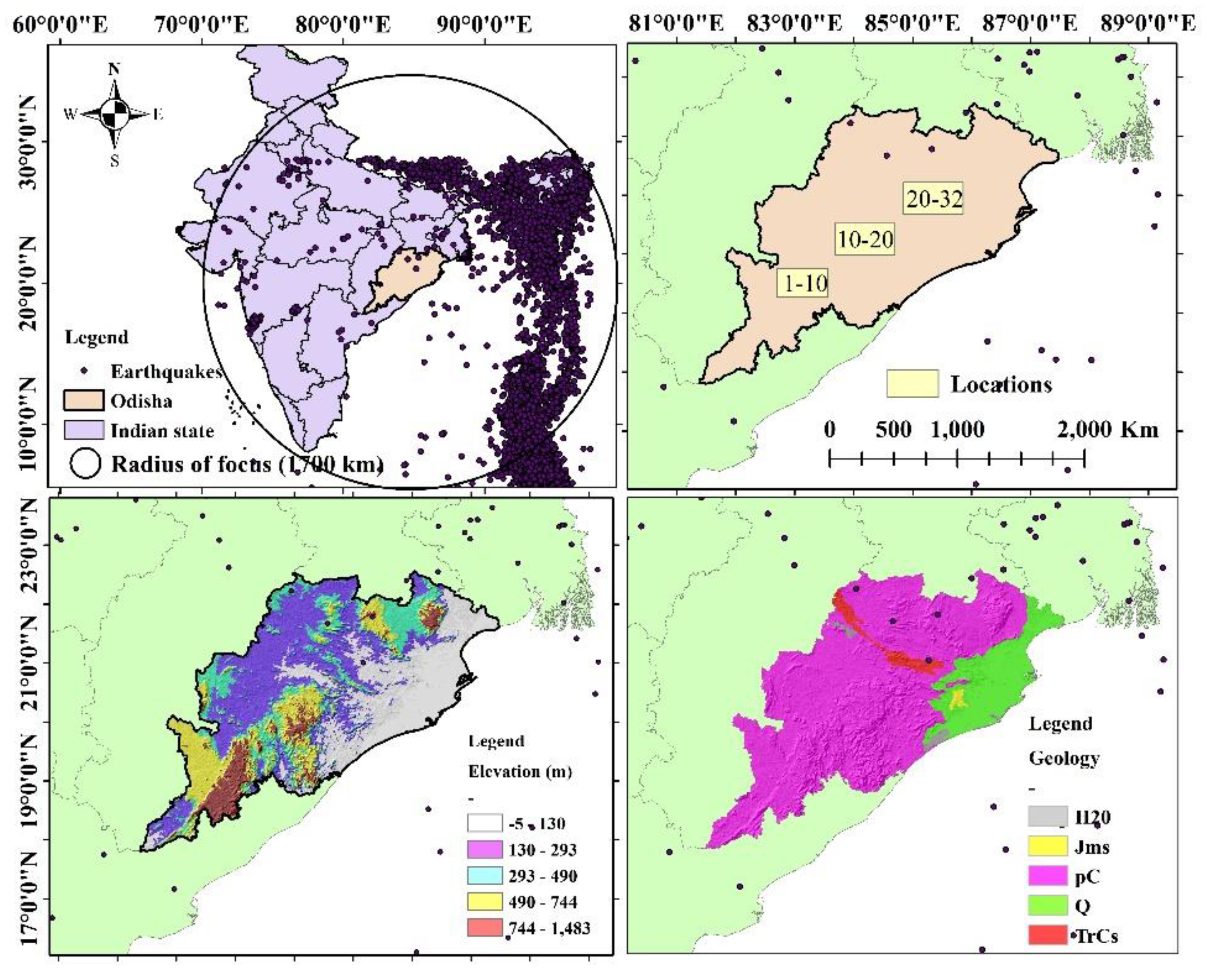
2.1. Study Area

Odisha is a state in eastern Indian and shares 450 km of coastline with the Bay of Bengal (Figure 1). The state is known for its tribal cultures, numerous hot springs, ancient history, and unique cultural and geographic environment. Odisha is situated between the latitudes of 17.780N and 22.730N, and longitudes of 81.37E and 87.53E. The capital of Odisha is Bhubaneswar, also called “temple city”. The state covers 155,707 km², which is approximately 4.87% of the total area of India. The population, according to 2019 census data, is approximately 4.6 million. Odisha’s GDP during this period (2017–18) was ₹4.16 lakh crore. According to the pre-existing seismic zonation map of India, Odisha comes under zones II and III.

Although much of Odisha is in zone II, Mahanadi graben is in zone III and encompasses cities such as Talchir, Angul, Bhubaneswar, Cuttack, Sambalpur, Dhenkanal, and the Balasore district. The Bonaigarh-Talchir area was struck by two moderate events (Mw 5 and 4.8) during May and June in 1995, respectively. Two more events also happened of 5.2 Mw in 1958 and 1962 within Rengali province. In January 1986, events of Mw 4.4, 4.1, and 4.3 were reported due to the active north Odisha boundary fault (NOBF), respectively. The Geological Survey of India established four stations for micro-earthquake measurement in the Bonaigarh–Talchir area. However, many hypocenters were observed in NOBF, indicating neo-tectonics.

2.2. Geological Settings

In this section, we describe a tentative geological setting in Odisha. Dating of rocks revealed that Odisha carries a 3700 million year (M.Y.) geological history [22]. Precambrian rocks cover 75% of Odisha. Accordingly, about 25% consists of Post-cambrian deposits, including unconsolidated sedimentary rocks [23]. The availability of basement rocks includes granites and gneisses, khondalites, charnockites, and ultrabasic-basic intrusions of granitic essence. The Eastern Ghats Mobile Belt (EGMB) is divided from North Odisha Craton (NOC) by the east-west running MSZ. Some observations have been conducted along the litho-contact between the cratons. The fault zone originated between the cratons, giving rise to Gondwana graben, and characterized by coal deposits. As the fault slices intermingle, the stratigraphic relation is difficult to interpret because of sedimentation, granitic intrusion, and lateritic cover concealing the contact.

EGMB is characterized by granulite-facies such as quartzites, charnockites khondalites, garnet-biotite schists, and gneisses. EGMB can be distinguished by the Rengali (northern fringe) and Angul (southern fringe) assemblages, even though they have different lithological characteristics. The North Orissa craton consists of a banded iron formation (BIF) and low-grade supracrustals within several generations of granitic intrusion [24]. EGMB rocks are believed to form before BIF-bearing granites. EGMB 1.0–0.8 Ga (Grenville-age) rocks formed because of several late Proterozoic events, include migmatization, alkali plutonism, and charnockitization. The fault and the litho-contact zones are characterized by nepheline syenite and ultrabasic rocks bearing chromite, respectively. Amphibolite facies can be found in the south of the Singhbhum craton [24]. Meta-sedimentary and meta-igneous rocks can be found in EGMB composed of migmatite [25]. Mahanadi graben is located in E–W orientation, which is sandwiched between EGMB and NOC. However, the basin is considered as a half-graben and comprises many stepwise normal faults with Gondwana deposits. Thus, NOBF trends parallel to EGMB structures in the direction of WNW–ESE and is found in between the NOC and Mahanadi basin. Kerajang fault is within the Talchir basin and situated along the NOBF. Moreover, MSZ and NOBF reactivation directs basin and seismicity tectonic development [26].

2.3. Data

Data collection from multiple sources were used in this study. Kolathayar et al. [27] designed spatial attenuation relationships that converted magnitudes scaled into a standardized moment scale. The body-wave magnitude (Mb) scale was used to estimate the magnitude of events in moment magnitude (Mw). In this study, a complete catalog of historical events was collected for probability mapping. The public and private disaster management agencies made earthquake catalogs freely available. The accessible sources were the Advanced National Seismic System (ANSS), United States Geological Survey (USGS), National Center for Seismology (NCS), and the National Earthquake Information Center (NEIC). The digital elevation model (DEM) and earthquake catalog from USGS were used to prepare a geodatabase and generate several layers for SSA and EPA. Geological data including the faults, lithology, and amplification factors for different rock types were used to generate indicators. Training and prediction of the classifications were performed for probability mapping. The raw geological map was collected from the Geological Survey of India (GSI) and applied to produce thematic layers. The seismotectonic atlas published by Geological Survey of India [23] was employed as an authentic referral for locating potential sources.

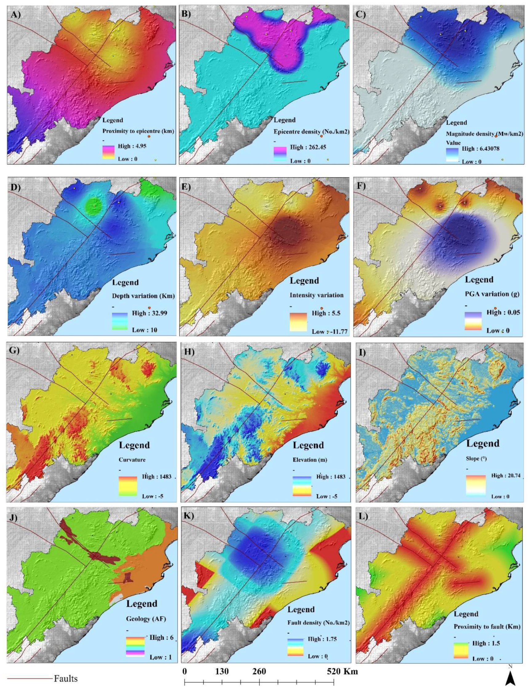
2.4. Thematic Layer Preparation

We conducted an extensive literature review. Choropleth maps were not developed in this study. The chorochromatic and cartogram maps were developed using ArcGIS statistical software (Version 10.4, Environmental Systems Research Institute (Esri), Brisbane, Australia). The probabilistic study is quite challenging, especially with regard to data-dependent models.

In this research, a 30 m spatial resolution DEM, geological data, estimated PGA, and intensity values were used to estimate causal factors. To prepare thematic layers, we implemented a world geodetic system (WGS) 1984 reference system. The derived thematic layers were elevation, slope, curvature, geology, fault density, Euclidean distance from faults, proximity to the epicenters, epicenters density, magnitude density, and depth variation (Figure 2). The obtained thematic layers of causal factors were presented in a stretched format.

Table 1. Raw data and input parameters used for assessments.

Assessment	Raw Data	Input Parameters	Methods	Resolution and Scale
Susceptibility to seismic amplification (SSA)	Digital elevation model (DEM) and geological information	Amplification factor elevation Slope curvature	Weighted overlay using predefined weights	30 m and 1:30,000
Earthquake probability assessment (EPA)	DEM, geological data, earthquake inventory, geo-structural information, attenuation relationship	Elevation slope Curvature magnitude density Depth density Epicenter density Proximity to epicenters Fault density Proximity to fault Geology	Recurrent neural network (RNN)

provides detailed data used in the current study. By uncovering objective themes, emerging patterns, and insight logic, these layers can be understood. Preprocessing, processing, and post-processing were conducted to estimate probability [28]. Layers were converted to multiple values by points and each pixel value was estimated. Some negative and unexpected values were removed from the database. Prediction of classification was conducted and then post-processing was performed after the testing task [6]. The predicted exact values of each pixel were post-processed to remove irrelevant pixel values. Until the end, the point-to-raster conversion was performed in a GIS environment, which generated SSA and EPM.

Importance of Factors

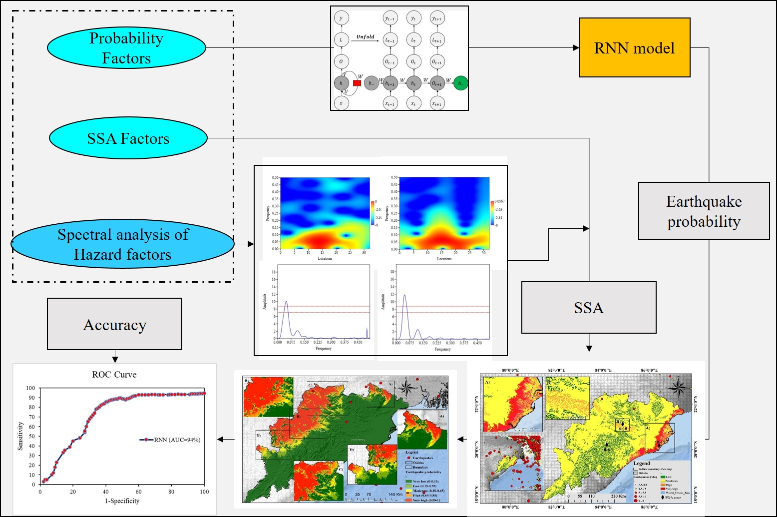
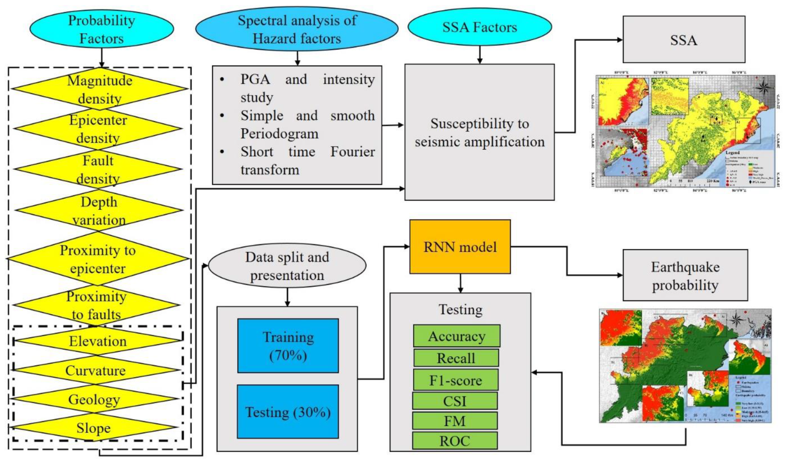
Slope and curvature [6,29]: Landscape processes are affected by slope structure. Several geomorphological processes such as subsurface flow velocity, erosion potential, runoff rates, and overland flow are most affected by slope characteristics. Slopes are associated with crustal faults. Moreover, fault length and size depends on the slope inclination angles. Curvature is associated with slopes having either a positive, negative, or zero curvature. Basins have negative curvatures and their locations for sedimentary deposits are susceptible to seismic amplification.

Elevation [30]: High elevation indicates erosion areas with complicated structures. The probability of earthquakes increases when elevation increases. Therefore, high-elevated areas (i.e., the Himalayan region) are extremely susceptible to earthquakes.

Fault density and proximity to faults: Earthquake probability increases when fault density also increases. Earthquake occurrence is high if faults are active in a complex tectonic condition.

Geology with amplification factor values [31]: Amplification factors of various rock types vary depending on composition. This information is useful to identify locations of high ground shaking.

Epicenter density and proximity to epicenter [32]: Earthquake events are clustered at a location and are high density. However, areas with large events are considered as zones of high probability. Earthquake probability is high when zones are clustered. Earthquake probability decreases when distance from an earthquake epicenter increases.

Magnitude and depth density [32]: Magnitude density indicates the likelihood of occurrence of a particular event. Density provides information for fault capacity and depth that could generate a particular magnitude event. The complex active fault system is more probable in areas that can produce high magnitude events.

2.5. Methodology

2.5.1. Spectral Analysis

Spectral analysis is popularly known as spectrum analysis, which plots the time-dependent spectrum of frequencies [33]. In seismology, the spectral analysis is generally conducted for seismic signal processing, through an algorithm that displays the power of different frequency elements for a time-domain signal. Therefore, this is also called frequency domain analysis in signal processing.

Signals are displayed in the form of a periodogram. A periodogram shows the spectral density with respect to frequency. Therefore, the periodogram for a sequence [x₁, ...., x_n] can be mathematically presented as:

$${\widehat{\varnothing }}_{\mathrm{p}}\left(\mathsf{\omega }\right)=\frac{1}{\mathrm{n}}{\left|{\displaystyle \sum }_{\mathrm{t}=1}^{\mathrm{n}}{\mathrm{x}}_{\mathrm{t}}{\mathrm{e}}^{-\mathrm{i}\mathsf{\omega }\mathrm{t}}\right|}^2$$

(1)

The expression presented in Equation (1) can form a power spectrum of any seismic signal having values of [x₁, ..., x_n], where $\mathrm{t}$ is time and n = 1,2,3… etc. The window $\left(\mathsf{\omega }\right)$ can be selected based on requirements. However, we implemented the Blackman window to improve continuous function. The power spectral density ${\widehat{\varnothing }}_{\mathrm{p}}\left(\mathsf{\omega }\right)/\mathrm{F}$ of a periodogram can be estimated using a nonuniform fast Fourier transform, where the frequency is 2π during no supply of the sampling frequency. However, the sampling frequency (fs) is applied when the frequency range is (0, 1). The main aim of the periodogram spectral estimator is to expose “hidden periodicities” in a time series analysis that defines the periodogram [34,35].

2.5.2. Short-Time Fourier Transform

In short-time Fourier transform (STFT) functions, if time is continuous, then a window function multiplied with the existing function cannot be zero [36]. The one-dimensional Fourier transform function can be converted into a two-dimensional signal when the function is filtered along the time axis. The expression can be mathematically presented as:

$$\mathrm{STFT}\left\{\mathrm{x}\left(\mathrm{t}\right)\right\}\left(\mathsf{\tau },\mathsf{\omega }\right)\equiv \mathrm{X}\left(\mathsf{\tau },\mathsf{\omega }\right)={\int }_{-\infty }^{\infty }\mathrm{x}\left(\mathrm{t}\right)\mathsf{\omega }\left(\mathrm{t}-\mathsf{\tau }\right){\mathrm{e}}^{-\mathrm{i}\mathsf{\omega }\mathrm{t}}\mathrm{dt}$$

(2)

where the window function is $\mathsf{\omega }\left(\mathsf{\tau }\right)$ and the Blackman window is centered throughout. However, the signal $\mathrm{x}\left(\mathrm{t}\right)$ needs to be transformed. Frequency is also represented by $\mathsf{\omega }$. The Fourier transform of $\mathrm{x}\left(\mathrm{t}\right)\mathsf{\omega }\left(\mathrm{t}-\mathsf{\tau }\right)$ is presented through function $\mathrm{X}\left(\mathsf{\tau },\mathsf{\omega }\right)$. Using the STFT function, the magnitude, signal frequency, and expected location can be plotted. The time index $\mathsf{\tau }$ is not presented as high resolution and is instead considered as “slow” time. In Equation (2), ${\mathrm{e}}^{-\mathrm{i}\mathsf{\omega }\mathrm{t}}$ is used to solve a differential equation, where $\mathrm{t}$ is time and $\mathsf{\omega }$ is frequency.

2.5.3. Estimation of Distance from Source-to-Site, PGA and Intensity

Joyner and Boore [37] developed the attenuation equation to calculate PGA. The required data for PGA estimation can be collected from the USGS earthquake catalog. Firstly, there is a requirement to calculate the source to site distance based on the epicentral distance according to the catalog, as presented in Equation (3). Similarly, the intensity values for each earthquake were estimated using Equation (5). Various researchers have proposed several attenuation equations, yet in this study we applied Joyner and Boore’s equation [37]. Source to site distance can be estimated based on the following:

$$\mathrm{D}=\left(\mathrm{E}^2+7.3^2\right)^0.5$$

(3)

where D = distance from the source to site and E = epicentral distance.

Joyner and Boore [37] presented the PGA estimation equation as:

$$\mathrm{PGA}=10^\left(0.249*\mathrm{M}-\mathrm{Log}\left(\mathrm{D}\right)-0.00255*\mathrm{D}-1.02\right)$$

(4)

where M = Earthquake magnitude. Many other attenuation laws can be implemented in a probabilistic seismic hazard assessment (PSHA) [38,39,40]. Boore and Joyner [37] developed the general equation of regression, which is popular for its regional and worldwide use. However, the modified Mercalli intensity (MMI) was calculated from PGA values using the proposed equation:

$$\mathrm{MMI}=1/0.3*(\log 10\left(\mathrm{PGA}*980\right)-0.014$$

(5)

where the PGA unit is G (Gal).

PGA variation and MMI variation were obtained for the 1800 events. Similarly, PGA and intensity variation were estimated for Odisha. We considered 32 locations from south to north that had a specific PGA value and intensity. All locations were chosen with STFT analysis and 32 was the minimum point to conduct the analysis. If we consider all values as peaks of a signal, then the PGA and intensity variation at all locations can be understood through STFT analysis. However, PGA and intensity variation were not involved in probability assessment, as these are hazard factors. In the next stage, seismic amplification mapping susceptibility conducted to identify high ground shaking locations.

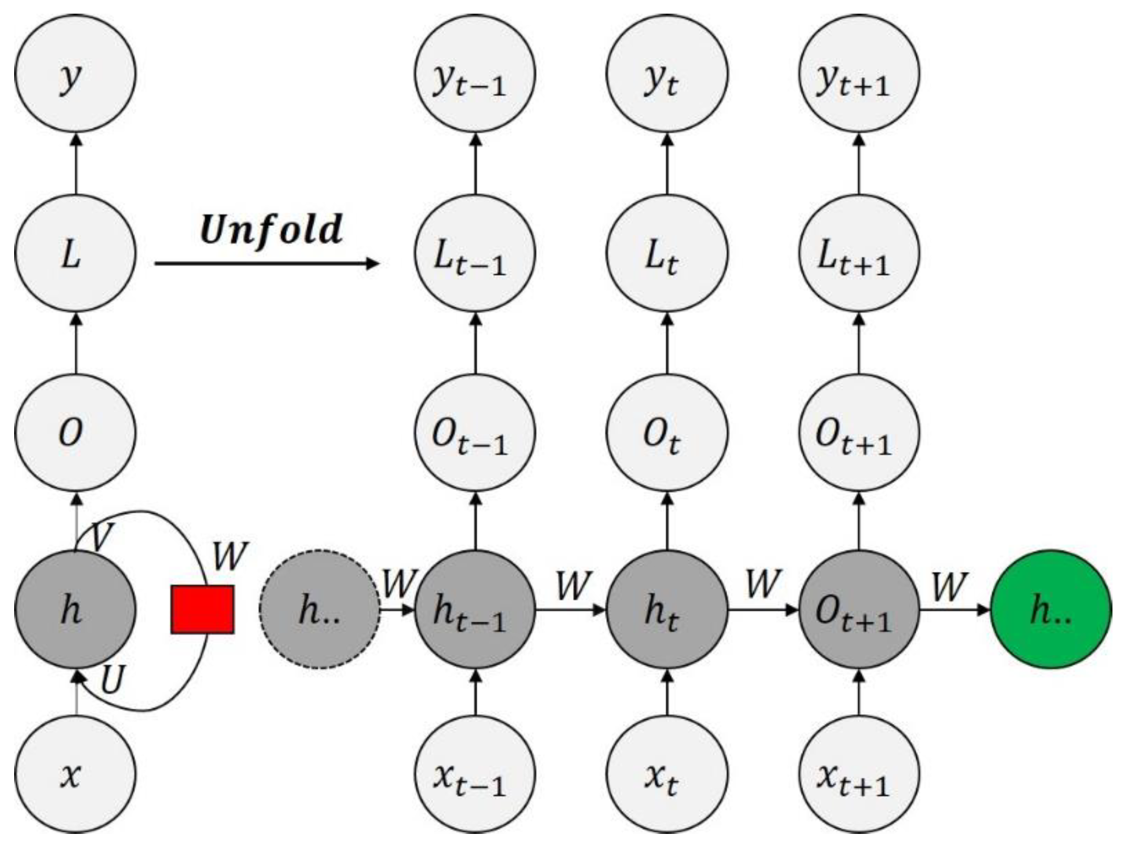
2.5.4. Recurrent Neural Network

RNN architecture is made up of input, hidden, and output layers that can process dynamic information. However, data must be in a serialized form and periodically connect to hidden nodes (Figure 3). In contrast to other neural networks, RNN follows the order of information. All the input and output values are independent in the traditional neural networks. However, in the RNN model, within the hidden layer inter-association among units occurred with different time intervals. Thus, through this process, information can pass away from one to another layer within the network [41].

The information shared across the RNN network precisely incorporates the concept of “loop feedback”. Similar to having a loopback in the Elman or Jordan network, this simple RNN model was implemented with a loopback. In this study, the RNN model consists of ${\mathrm{x}}_{\mathrm{t}}$ as input, ${\mathrm{h}}_{\mathrm{t}}$ as hidden, and ${\mathrm{y}}_{\mathrm{t}}$ as the output vector at time t. Therefore, the expressions can be presented as follows:

$${\mathrm{h}}_{\mathrm{t}}=\mathsf{\sigma }\left({\mathrm{W}}_{\mathrm{h}}{\mathrm{x}}_{\mathrm{t}}+{\mathrm{U}}_{\mathrm{h}}{\mathrm{h}}_{\mathrm{t}-1}+{\mathrm{b}}_{\mathrm{h}}\right)$$

(6)

$${\mathrm{y}}_{\mathrm{t}}=\mathsf{\sigma }\left({\mathrm{W}}_{\mathrm{y}}{\mathrm{h}}_{\mathrm{t}}+{\mathrm{b}}_{\mathrm{y}}\right)$$

(7)

where parameter matrices are W and U, $\mathsf{\sigma }(\cdot )$ is represented as loss function of the training sample sequence, and the bias vector b.

2.5.5. Data Presentation for RNN

Detailed RNN model parameters are presented in

Table 2. RNN model parameters and importance.

Optimized Parameter	Suitable Values for RNN	Description
Epoch	100	100 times train the sample
Batch size	64	Size of each data batch
Drop out	0	Reduce overfitting
Optimizer	Adam	Adaptive moment estimation
Learning rate	Cross-entropy	Used for binary classification
Loss function	0.001	Weight updating speed

. In this study, all the 10 thematic layers were converted into data points to explore the RNNs predictive potential. The experienced earthquakes were presented for RNNs. Firstly, each probability indicator was selected in a sequence. However, each layer can be regarded as a single-band image. Every layer was stacked in an Excel sheet. Then, using the information to gain the algorithm, factor importance was estimated. According to the importance, the sequence was as follows: magnitude density, epicenter density, fault density, depth variation, proximity to the epicenter, distance from the faults, elevation, curvature, geology, and slope. Dara were organized in a sequence in descending order of significance.

Each pixel value must be converted to a sequential sample. Accordingly, in the RNN model, the most valuable factors were sent first and the least valuable factors were sent last. Moreover, because of the recurrent structure, critical information was retained and proceeded to the hidden state, thus predicting earthquake (1) and non-earthquake (0) targets. Figure 4 presents this methodological flowchart.

2.5.6. Model Evaluation Methods

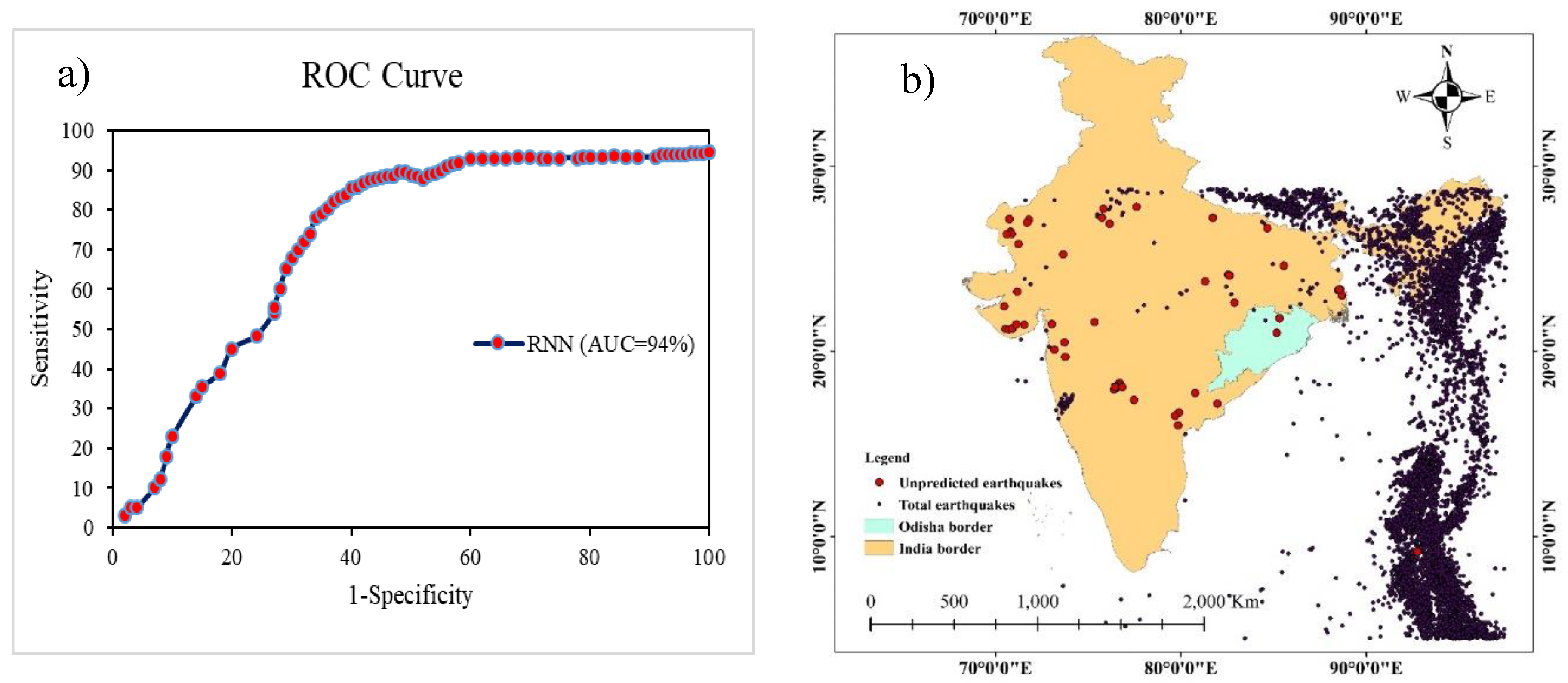
To assess the proposed model, evaluation techniques were used [42]. The diagnostic ability of the model was represented by the ROC. The ROC portrayed the specificity curve against sensitivity. The area under the curve (AUC) depicted the prediction values. The prediction was better when the area under the curve was larger [43]. The prediction ability of RNN model was determined based on ACC, recall, F1-score, precision, threat score (TS), CSI, and FM, and can be expressed as follows [44,45,46]:

$$\mathrm{ACC}=\frac{\mathrm{TP}+\mathrm{TN}}{\mathrm{TP}+\mathrm{FP}+\mathrm{TN}+\mathrm{FN}}$$

(8)

$$\mathrm{Recall}=\frac{\mathrm{TP}}{\mathrm{TP}+\mathrm{FN}}$$

(9)

$$\mathrm{F}1\mathrm{score}=\frac{2\times \mathrm{TP}}{2\times \mathrm{TP}+\mathrm{FP}+\mathrm{FN}}$$

(10)

$$\mathrm{Precision}=\frac{\mathrm{TP}}{\mathrm{TP}+\mathrm{FP}}$$

(11)

$$\mathrm{CSI}=\frac{\mathrm{TP}}{\mathrm{TP}+\mathrm{FN}+\mathrm{FP}}$$

(12)

$$\mathrm{FM}=\sqrt{\frac{\mathrm{TP}}{\mathrm{TP}+\mathrm{FN}}·\frac{\mathrm{TP}}{\mathrm{TP}+\mathrm{FP}}}$$

(13)

Hereby, true positive (TP) and true negative (TN) show the correct classification of earthquakes and non-earthquakes. Similarly, false-positive (FP) and false-negative (FN) indicate misclassified earthquakes and non-earthquakes, respectively. For accuracy, the values of every statistical performance must be between 0 and 1. Moreover, the higher the ACC performance values, recall, F1-score, and CSI, the better the model works (

Table 3. Confusion matrix of prediction based on RNN.

		Predicted
		Positive	Negative
Actual	Positive	1750	50
	Negative	100	800
		Accuracy	0.94
		Precision	0.95
		Recall	0.97
		F1 score	0.96
		Threat score (TS) or critical success index (CSI)	0.92
		Fowlkes–Mallows index (FM)	0.95

). Moreover, MCC value were estimated for perfect predictions (1), random predictions (0), and inconsistency (1).

3. Results

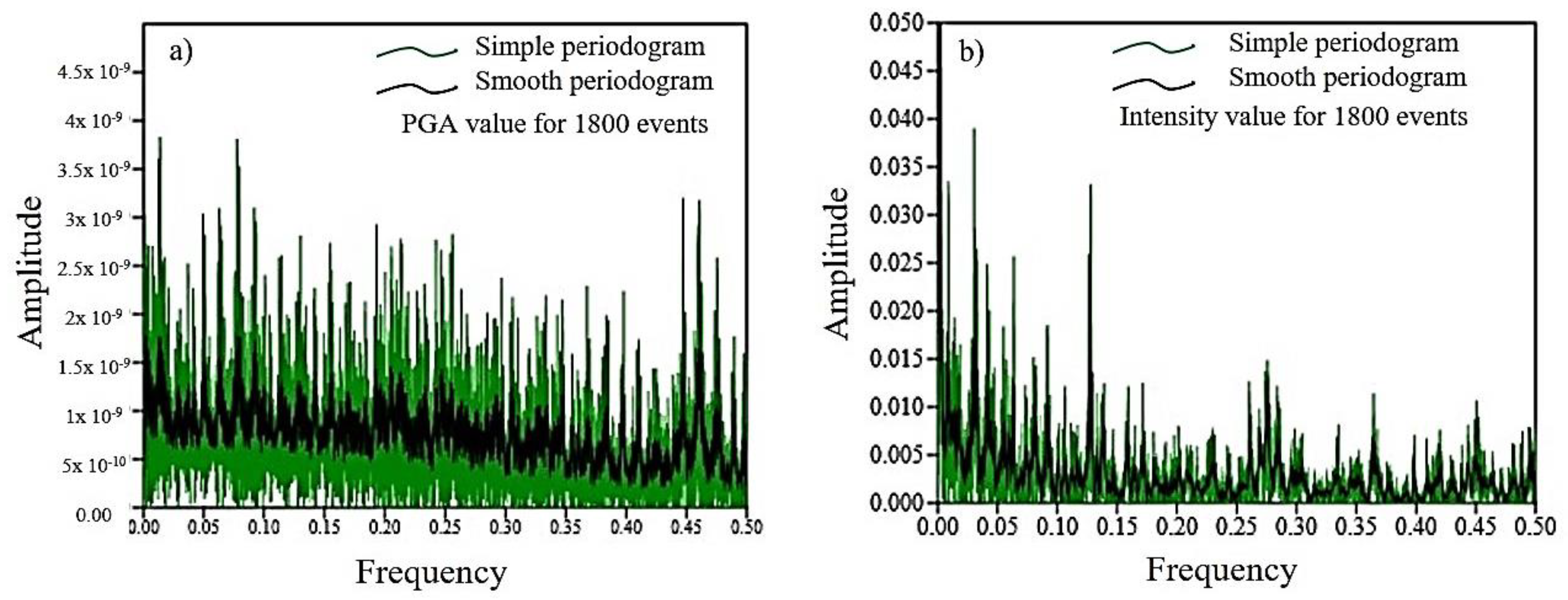
3.1. Periodogram Plotting of PGA and Intensity

In seismology, periodogram represents seismic signal spectral density. However, in this study, the PGA power spectra (amplitude) and intensity were plotted against the frequency based on the Hamming window (green color, Figure 5). Therefore, having a radius of 1700 km kept Odisha ay the center and 1800 events were implemented to plot the periodogram. No recorded wave signal was used to perform the periodogram study. Amplitudes were observed against frequencies for all PGA and intensity values. By averaging the frequency, a smoothed periodogram was plotted in a black color instead of time. The spectral plot of the smoothed periodogram shows the highest amplitude of PGA at the frequency of 0.01, while the highest amplitude of intensity is at the frequency of 0.04. High amplitude with low frequency provides information regarding controlling earthquakes.

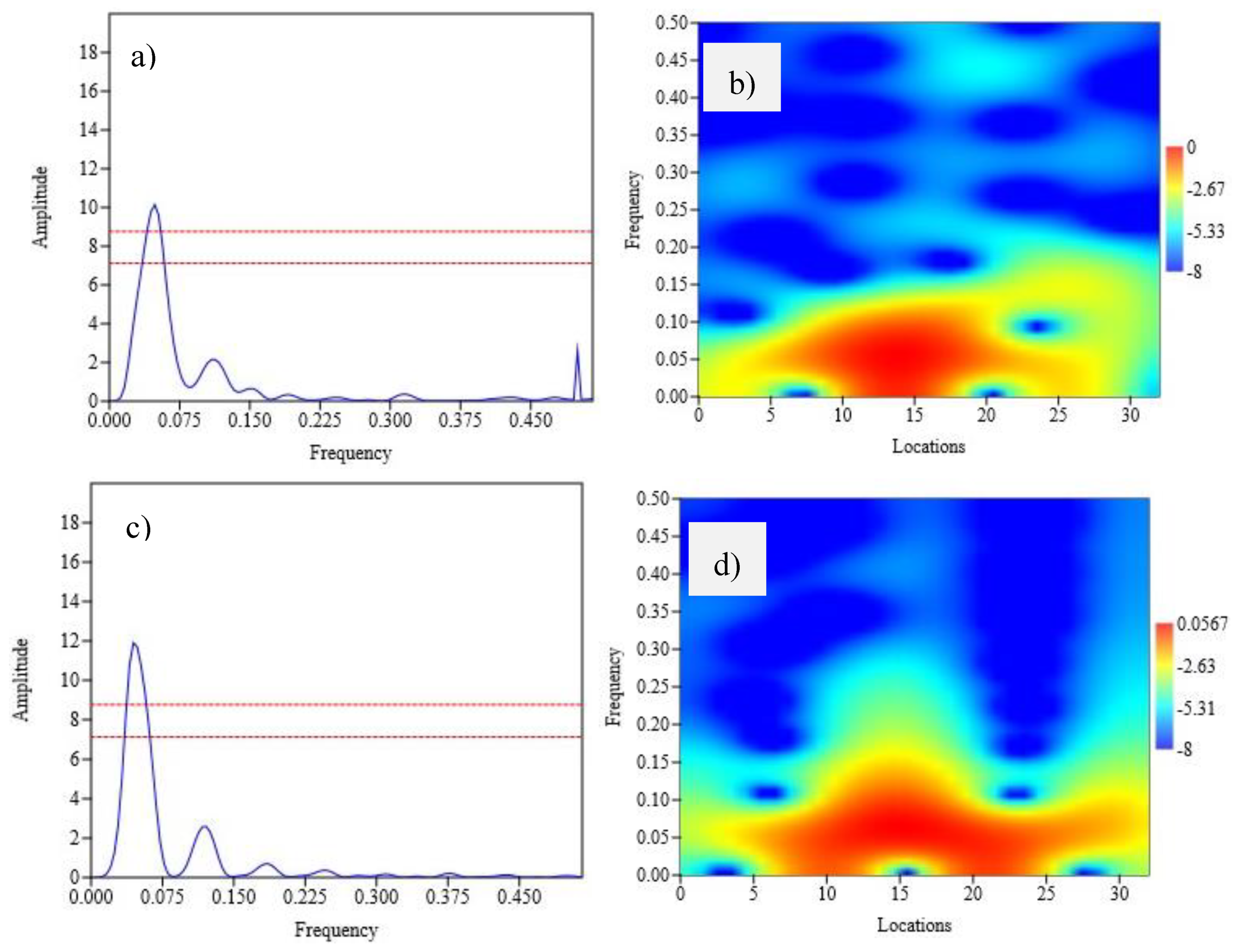
3.2. Short-Time Fourier Transform

PGA (0–0.53 g) and intensity (II to VI) variations were observed in Odisha. Periodogram of the spectral density of PGA and intensity variations were plotted for the study area. In Figure 6a, the amplitudes of PGA values are shown against frequency, where the amplitudes vary from 0–10 m, while frequencies vary from 0–0.5 Hz. Similarly, in Figure 6c, the amplitudes of intensities vary from 0–12 m, while frequencies vary from 0–0.5 Hz. However, in both cases, the amplitude level at the frequency of 0.01 is 8.76 Hz, while the amplitude level at the frequency of 0.05 is 7.129 Hz. This indicates that the power of the amplitude increased when frequency decreased. Therefore, the highest PGA and intensity can be expected in Cuttack, Bhubaneswar, Kendrapada, Jagatsngpur, Puri, Khordha, Anugul, Dhenkanal, and some parts of Bhadrakh and Baleswar. STFT simulation was conducted using the Blackman-Harris window, which had a window size of 512 mm (rectangular window = 512). STFT analysis for PGA and intensity in the simulated graph have a stretched magnitude. In Figure 6b, the frequencies of PGAs are plotted against 32 expected locations. The locations were chosen randomly. PGA variation in Odisha was highest between the location of 10–18, where frequency varied from 0–0.1 Hz. STFT simulation for intensity variation was projected for 32 locations in Odisha, as shown in Figure 6d. The highest intensity could be expected at the locations from 7–14 and 17–25, having a frequency range of 0–0.15 m. The highest PGA and intensity were observed in Cuttack, Bhubaneswar, Anugul, Dhenkanal, and some parts of Bhadrakh and Baleswar. This analysis did not count external factors of sub-surface lithology and complicated tectonic structures. Therefore, SSA was conducted to identify the expected locations for high ground shaking.

3.3. Susceptibility to Seismic Amplification (SSA)

The study area falls within seismic zones II and III. Therefore, SSA results obtained from this study are not surprising, as they follow seismic zones (Figure 7). However, PGA observed in this study ranges between 0–0.53 g, which was implemented after SSA and could reach up to 0.092 g. According to the obtained results, the highest intensity could reach up to VI with the highest PGA value of 0.092–0.18g, which was determined by considering several factors, such as amplification factors of rock types, slope, location elevation, and recent sediments in the basin. The highest velocity of the surface waves could reach up to 8.1–16 (cm/s). This gives an indication of strong ground shaking. The shaking was strong despite the potential damage ranging from light to moderate. The highest ground shaking was observed in coastal Odisha and Mahanadi graben. Moderate shaking was observed in the IB river basin, Talchir basin, and Jajpur-Chandbali basin situated in the northwestern part, while Athgarh and Salepur basins are on the southern part of the Mahanadi rift valley. The seismic ground velocity divides the state into three major parts: 0–6, 6–10 and 10–15 cm/s. The final map was classified into four classes of very high, high, moderate, and low ground shaking. The east coast of the Mahanadi river basin and coastal parts of the Bay of Bengal basin, including Chilika Lake, have very high ground shaking. The cities with very high-to-high susceptible areas are Ganjam, Puri, Jagatsinghpur, Kendrapada, Bhadrakh, and Baleswar, as well as some parts of Khordha, Cuttack, and Jaipur. In the moderate ground shaking category are Dhenkanal, Anugul, Sambalpur, and Jharsuguda. In addition, all other districts fall in the low category.

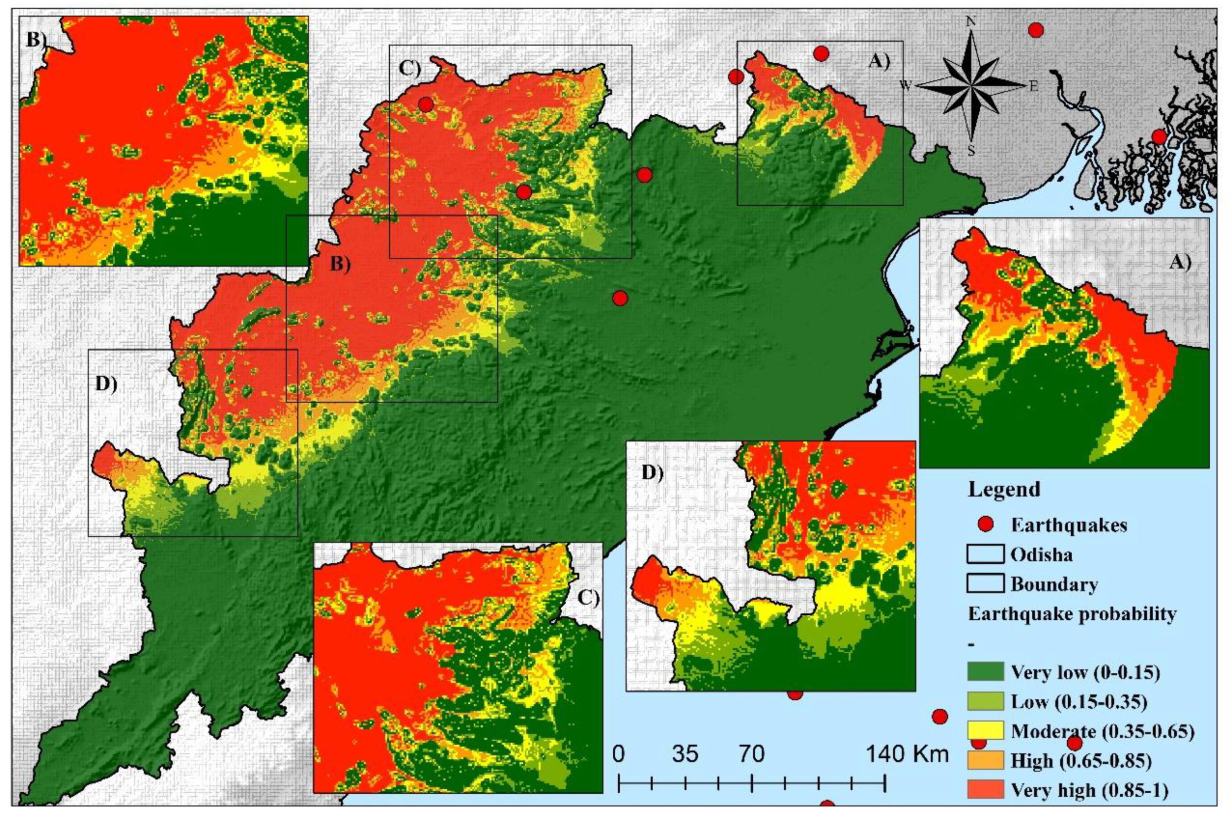
3.4. Earthquake Probability Assessment

A probability assessment was conducted using the RNN model to predicts earthquake (1) and non-earthquake (0) classifications. The model was unable to predict 50 earthquake data points out of 1800 events. Due to heterogeneity and irrelevant values obtained for some pixels in the thematic layers, the model predicted 1750 events out of 1800 events. In total, 1850 points were predicted as earthquakes, while 850 were non-earthquakes. The RNN model predicted 48900 km² as the highest earthquake probable location in Odisha. Training (70%) and testing (30%) were conducted for 2700 points, where 1800 were earthquakes and 900 were non-earthquakes. The RNN model achieved 94% accuracy. The accuracy was estimated as 0.94, whereas as precision was 0.94, recall was 0.97, F1 score was 0.96, TS/CSI was 0.921053, and FM was 0.95. The probability map is presented in Figure 8. Accuracy is plotted through ROC (Figure 9a) and every true negative event is plotted in Figure 9b. All unpredicted earthquakes showed no discernible pattern.

The probability of future earthquake occurrence is higher in the northwestern parts of the state, as shown in Figure 8. However, the northwestern part of Odisha has already experienced moderate magnitude events of 5.3 Mw due to the NOBF active fault system. Four sections of the very high probable areas were shown within the map, showing that NOBF has the capability to strike high magnitude events in the future. NOBF extends from the east to the west, having a strike length of 250 km, whereas width ranges from 2–5 km. The NOBF is not uniform and is rather characterized by interdigitation of rocks, which makes northern Odisha irregular with complex geo-structures. Therefore, high probability in the northwestern and southern Odisha can be associated with NOBF. Medium probability was characterized as having high probability, whereas low probability could be expected in east and central Odisha. The districts under very high (0.85–1) to high (0.65–0.85) probability includes Sundargarh, Jharsuguda, Sambalpur, Bargarh, Subarnapur, Balangir, Nuapada, Kalahandi, and Nabarangpur. All other districts fall in the moderate to very low categories. Approximately 33.46% and 52,014 km² of Odisha fall in the very high to high category (

Table 4. Area under earthquake probability in Odisha.

Class no.	Class	Area (km2)	Area (%)
5	Very-high	48,900	31.4
4	High	3204	2.06
3	Moderate	3603	2.31
2	Low	493	0.32
1	Very-low	99,507	63.9
Total		155,707	100

).

4. Discussion

SSA indicates that eastern coastal districts in Odisha are highly susceptible to amplification. This is because of the widespread deposits of unconsolidated sediments with nonuniform thickness in association with low groundwater levels. The SSA map obtained from this study considered slope (35%), curvature (32%), elevation (23%), and lithology with amplification factors (10%) as the conditioning factors with predefined weights [47]. According to the periodogram and STFT simulation, the PGA ranged between 0–0.9, whereas the PGV ranged between 0–15 (cm/s). The districts with a velocity of 0–3 (cm/s) are Rayagada, Kandhamal, Ganjam, Gajapati, and Keonjhar. This demonstrates that lower PGA values could be attributed to less complicated structural features, with strong basement and rock types. The areas with PGVs between 6 to 10 (cm/s) are the major basins of Odisha, including the Mahanadi basin, where there are thick unconsolidated layers of deposits. However, the highest PGV was observed in the eastern coastal districts, ranging from 10–15 (cm/s). This is due to the Mahanadi river delta and Brahmani river delta, as well as the Bay of Bengal basin. The northern and central parts of Odisha accommodates the Talchir basin, Rengali Province, and IB basin at the north of EGMB, all of which fall under moderate PGA characterized by larger structural faults. Several studies on seismic microzonation [47,48,49] have explained ground shaking. Yet few researchers have employed litho-dynamic, stratigraphic, and topographic influencing factors when assessing ground-shaking amplification [50]. Moreover, Aucelli et al. [51] used geological and geomorphological factors to estimate the susceptibility index for seismic amplification in Italy. Therefore, Odisha is seismically active because of periodical NOBF reactivation. Therefore, the next step probability assessment was conducted to show the highest probability in northwestern Odisha.

The probability map was obtained from the study denotes a very high to high probability in the northwestern parts of the state and decreases towards the central and coastal areas. There is a transition zone of moderate to low probability in between that can be perceived. However, all earthquakes in Odisha are intraplate shallow-focus earthquakes. Mahanadi graben is situated as an interior active region of Odisha that is relatively stable compared to the Himalayan region and Java Sumatra subduction zone. Clustering of earthquakes gives a pattern with foreshocks, mainshocks, and aftershocks, which were not studied in this work, as not many events like this experienced in Odisha. Furthermore, earthquakes do not always follow patterns, which makes it less common to estimate probability. Mostly, a significant number of earthquakes originated at shallow depths of 70 km within the state, while deep-focus earthquakes were experienced within the Bay of Bengal. Therefore, the leading cause of probability in Odisha could be the active NOBF system. As we observed, the seismic amplification was higher in the Mahanadi graben and coastal parts of Odisha, experiencing a few small-magnitude events. Therefore, the coastal parts are not highly probable for future events because of less complicated structural features, low height, and more sediments than stressed rocks. Moreover, some specific areas are prone to swarms, such as geothermal areas, including hot spring locations. However, in Odisha, hot springs are associated with the Mahanadi Shear Zone, which is not presently active. Sometimes, a particular location has several small earthquakes before a larger event. Therefore, we believe that the events in western Odisha could be the foreshock. However, these events do not look like foreshocks and cannot be considered as such until overtaken by mainshocks. In addition, earthquake size is dependent on fault type, length, depth, and fault slip. Recently, scientists have tried to predict earthquakes based on clusters, as they could be a warning sign for a larger earthquake. Rout and Nanda [52] conducted a PSHA at Bhubaneswar and estimated spectral acceleration as 0.05 g if a high magnitude event hit the city. Mandal et al. [53] conducted a PSHA for central India and showed that the western Odisha is seismically active. According to the United Nations Development Program [54], faulted Mahanadi basin could be a potential source for future events. Odisha has not had a solid probability assessment. However, hybrid intelligent machine learning-based techniques have been developed for the potential zone and risk assessment [55,56]. Jena and Pradhan [57] described active tectonics and fault characteristics before the probability and risk assessment.

5. Conclusions

The present study proposed an RNN model for earthquake probability mapping in Odisha, India. The use of artificial intelligence and GIS in earthquake studies adds a new, beneficial dimension. Therefore, this work developed a SSA and EPM map based on the RNN classification technique, using direct attributes of pertinent criteria. This study demonstrated that the spatial variation of seismic amplification was very high in coastal parts of Odisha and high in the Mahanadi basin. Similarly, the probability map shows that very high-to-high probable locations for future events could be found in the western part of the state. The probability results denoted that structural attributes and complex geological/geomorphological features in western NOBF could be the main reason for high probability. However, a noticeable intersection of faults in the shear zone could have control on isoseismic elongation in the west. The study also shows the Mahanadi graben spreading and creating a huge basin for recent deposits. Hence, the active graben can damage the cities when originate from NOBF and the Bay of Bengal faults.

The RNN model was applied to transfer areas with similar or more complex tectonics and had several limitations. The proposed model and data analysis can cover a large study area but the process is time-consuming. This study can be considered as a reconnaissance study prior to performing a detailed study for mitigation and micro-zonation purposes. The RNN model deals with technical complexities and data uncertainties during the priority analyses. These processes can be modified and improved using integrated and ensemble techniques. The RNN model strictly depends on sequence, quality, and input data preparation.

Future works can be done in association with geophysical, seismological, geo-structural, geological, and earthquake engineering data, including novel integrated, hybrid, and ensemble techniques. Currently, remote sensing techniques and artificial intelligence techniques are popular and thus there is potential for a future project that uses high-resolution LiDAR techniques and images. In conclusion, the proposed model enables planners, managers, agencies, and policymakers to make decisions for land use planning, as well as scheming appropriate proposals for seismically active areas.

References

1. Gupta, S.; Mohanty, W.K.; Mandal, A.; Misra, S. Ancient terrane boundaries as probable seismic hazards: A case study from the northern boundary of the Eastern Ghats Belt, India. Geosci. Front. 2014, 5, 17–24. [Google Scholar] [CrossRef] [Green Version]
2. Kumar, T.S.; Mahendra, R.; Nayak, S.; Radhakrishnan, K.; Sahu, K. Coastal Vulnerability Assessment for Orissa State, East Coast of India. J. Coast. Res. 2010, 263, 523–534. [Google Scholar] [CrossRef]
3. Mahala, S.C. Geology, Chemistry and Genesis of Thermal Springs of Odisha, India. Springer Briefs Earth Sci. 2019, 5, 1572–1577. [Google Scholar] [CrossRef]
4. Rajendran, C.P.; Rajendran, K.; John, B. The 1993 Killari (Latur), central India, earthquake: An example of fault reactivation in the Precambrian crust. Geol. 1996, 24, 651. [Google Scholar] [CrossRef]
5. Di Giulio, G.; The L’Aquila Experiment Team; Marzorati, S.; Bergamaschi, F.; Bordoni, P.; Cara, F.; D’Alema, E.; Ladina, C.; Massa, M. Local variability of the ground shaking during the 2009 L’Aquila earthquake (April 6, 2009—Mw 6.3): The case study of Onna and Monticchio villages. Bull. Earthq. Eng. 2011, 9, 783–807. [Google Scholar] [CrossRef]
6. Jena, R.; Pradhan, B.; Beydoun, G.; Nizamuddin; Ardiansyah; Sofyan, H.; Affan, M. Integrated model for earthquake risk assessment using neural network and analytic hierarchy process: Aceh province, Indonesia. Geosci. Front. 2020, 11, 613–634. [Google Scholar] [CrossRef]
7. Ehret, D.; Hannich, D. Seismic Microzonation based on geotechnical Parameters-Estimation of Site Effects in Bucharest (Romania). AGUFM 2004, 2004, S43A-0972. [Google Scholar]
8. Theilen-Willige, B. Detection of local site conditions influencing earthquake shaking and secondary effects in Southwest-Haiti using remote sensing and GIS-methods. Nat. Hazards Earth Syst. Sci. 2010, 10, 1183–1196. [Google Scholar] [CrossRef]
9. Levchenko, O.V. Tectonic aspects of intraplate seismicity in the northeastern Indian Ocean. Tectonophys. 1989, 170, 125–139. [Google Scholar] [CrossRef]
10. Rai, A.; Tripathy, S.; Sahu, S. The May 21 st, 2014 Bay of Bengal earthquake: Implications for intraplate stress regime. Curr. Sci. (00113891) 2015, 108. [Google Scholar]
11. Bhatia, S.C.; Kumar, M.R.; Gupta, H.K. A probabilistic seismic hazard map of India and adjoining regions. Ann. Geophys. 1999, 42. [Google Scholar] [CrossRef]
12. Parvez, I.; Vaccari, F.; Panza, G.F. A deterministic seismic hazard map of India and adjacent areas. Geophys. J. Int. 2003, 155, 489–508. [Google Scholar] [CrossRef]
13. Jaiswal, K.; Sinha, R. Probabilistic Seismic-Hazard Estimation for Peninsular India. Bull. Seism. Soc. Am. 2007, 97, 318–330. [Google Scholar] [CrossRef] [Green Version]
14. Raghukanth, S.T.G.; Iyengar, R.N. Seismic hazard estimation for Mumbai city. Curr. Sci. 2006, 91, 1486–1494. [Google Scholar]
15. Anbazhagan, P.; Vinod, J.S.; Sitharam, T. Probabilistic seismic hazard analysis for Bangalore. Nat. Hazards 2008, 48, 145–166. [Google Scholar] [CrossRef]
16. Cornell, C.A. Engineering seismic risk analysis. Bull. Seism. Soc. Am. 1968, 58, 1583–1606. [Google Scholar]
17. Atkinson, G.M.; Boore, D.M. Earthquake Ground-Motion Prediction Equations for Eastern North America. Bull. Seism. Soc. Am. 2006, 96, 2181–2205. [Google Scholar] [CrossRef]
18. Petersen, M.D.; Mueller, C.S.; Moschetti, M.P.; Hoover, S.M.; Llenos, A.L.; Ellsworth, W.L.; Michael, A.J.; Rubinstein, J.L.; McGarr, A.F.; Rukstales, K.S. Seismic-Hazard Forecast for 2016 Including Induced and Natural Earthquakes in the Central and Eastern United States. Seism. Res. Lett. 2016, 87, 1327–1341. [Google Scholar] [CrossRef] [Green Version]
19. Wang, J.; Brant, L.; Wu, Y.-M.; Taheri, H. Probability-based PGA estimations using the double-lognormal distribution: Including site-specific seismic hazard analysis for four sites in Taiwan. Soil Dyn. Earthq. Eng. 2012, 42, 177–183. [Google Scholar] [CrossRef]
20. Keeney, R.L.; Raiffa, H. Decisions with Multiple Objectives: Preferences and Value Trade-Offs; Cambridge University Press: Cambridge, UK, 1993. [Google Scholar]
21. Mohanty, W.K.; Walling, M.Y.; Vaccari, F.; Tripathy, T.; Panza, G.F. Modeling of SH- and P-SV-wave fields and seismic microzonation based on response spectra for Talchir Basin, India. Eng. Geol. 2009, 104, 80–97. [Google Scholar] [CrossRef]
22. Sarkar, S.; Saha, A. Structure and Tectonics of the Singhbhum-Orissa Iron Ore Craton, Eastern India. In Structure and Tectonics of Precambrian Rocks of India; 1983; pp. 1–25. Available online: http://pascal-francis.inist.fr/vibad/index.php?action=getRecordDetail&idt=9063125 (accessed on 20 February 2020).
23. India, G.S.o.; Dasgupta, S.; Narula, P.; Acharyya, S.; Banerjee, J. Seismotectonic atlas of India and Its Environs; Special Publication Series 59; Geological Survey of India: Calcutta, India, 2000. [Google Scholar]
24. Mahalik, N. Geology of the contact between the Eastern Ghats Belt and North Orissa Carton, India. J. Geol. Soc. India 1994, 44, 41–51. Available online: https://ci.nii.ac.jp/naid/10007644438/ (accessed on 25 February 2020).
25. Gupta, S. Strain localization, granulite formation and geodynamic setting of ‘hot orogens’: A case study from the Eastern Ghats Province, India. Geol. J. 2011, 47, 334–351. [Google Scholar] [CrossRef]
26. Mukhopadhayay, A.; Chaudhuri, P.; Banerji, A. Contemporaneous intrabasinal faulting in Gondwana basin—The Jurabaga fault of Ib River Coalfield, a type example. J. Geol. Soc. India 1984, 25, 557–563. [Google Scholar]
27. Kolathayar, S.; Sitharam, T.G.; Vipin, K.S. Deterministic seismic hazard macrozonation of India. J. Earth Syst. Sci. 2012, 121, 1351–1364. [Google Scholar] [CrossRef] [Green Version]
28. Iyengar, R.N.; Kanth, S.T.G.R. Attenuation of Strong Ground Motion in Peninsular India. Seism. Res. Lett. 2004, 75, 530–540. [Google Scholar] [CrossRef]
29. Jena, R.; Pradhan, B. Integrated ANN-cross-validation and AHP-TOPSIS model to improve earthquake risk assessment. Int. J. Disaster Risk Reduct. 2020, 101723. [Google Scholar] [CrossRef]
30. Alizadeh, M.; Ngah, I.; Hashim, M.; Pradhan, B.; Pour, A.B. A Hybrid Analytic Network Process and Artificial Neural Network (ANP-ANN) Model for Urban Earthquake Vulnerability Assessment. Remote. Sens. 2018, 10, 975. [Google Scholar] [CrossRef] [Green Version]
31. Bathrellos, G.; Skilodimou, D.; Chousianitis, K.; Youssef, A.; Pradhan, B. Suitability estimation for urban development using multi-hazard assessment map. Sci. Total. Environ. 2017, 575, 119–134. [Google Scholar] [CrossRef]
32. Soe, M.; Ryutaro, T.; Ishiyama, D.; Takashima, I.; Charusiri, K.W.-I.a.P. Remote sensing and GIS based approach for earthquake probability map: A case study of the northern Sagaing fault area, Myanmar. J. Geol. Soc. Thailand 2009, 1, 29–46. [Google Scholar]
33. Burtin, A.; Bollinger, L.; Vergne, J.; Cattin, R.; Nábělek, J.L. Spectral analysis of seismic noise induced by rivers: A new tool to monitor spatiotemporal changes in stream hydrodynamics. J. Geophys. Res. Space Phys. 2008, 113, 5. [Google Scholar] [CrossRef] [Green Version]
34. Visalakshmi, G.; Praveen, I.; Ramesh, K.; Rao, S.K.; Bharathi, V.L. Power spectrum Estimation of Seismic Wave using Periodogram method. Int. J. Pure Appl. Math. 2017, 114, 191–199. [Google Scholar]
35. Schuster, A.; Hemsalech, G. VI. On the constitution of the electric spark. Philos. Trans. R. Soc. London. Ser. A Contain. Pap. a Math. or Phys. Character (1896-1934) 1900, 193, 189–213. [Google Scholar] [CrossRef]
36. Lu, W.; Li, F. Seismic spectral decomposition using deconvolutive short-time Fourier transform spectrogram. Geophysics. 2013, 78, V43–V51. [Google Scholar] [CrossRef]
37. Joyner, W.; Boore, D.M.; Porcella, R. Peak horizontal acceleration and velocity from strong motion records including records from the 1979 Imperial Valley, California, earthquake. Open-File Report 1981, 71, 2011–2038. [Google Scholar] [CrossRef]
38. Boore, D.M.; Joyner, W.B. The empirical prediction of ground motion. Bull. Seism. Soc. Am. 1982, 72, S43–S60. [Google Scholar]
39. Campbell, G.S. Soil Physics with BASIC: Transport Models for Soil-Plant Systems, 1st ed.; Elsevier: Oxford, UK, 1985; Volume 14. [Google Scholar]
40. Fukushima, Y.; Tanaka, T. A new attenuation relation for peak horizontal acceleration of strong earthquake ground motion in Japan. Bull. Seism. Soc. Am. 1990, 80, 757–783. [Google Scholar]
41. Xu, S.; Niu, R. Displacement prediction of Baijiabao landslide based on empirical mode decomposition and long short-term memory neural network in Three Gorges area, China. Comput. Geosci. 2018, 111, 87–96. [Google Scholar] [CrossRef]
42. Wang, Y.; Fang, Z.; Wang, M.; Peng, L.; Hong, H. Comparative study of landslide susceptibility mapping with different recurrent neural networks. Comput. Geosci. 2020, 138, 104445. [Google Scholar] [CrossRef]
43. Tsangaratos, P.; Ilia, I.; Hong, H.; Chen, W.; Xu, C. Applying Information Theory and GIS-based quantitative methods to produce landslide susceptibility maps in Nancheng County, China. Landslides 2016, 14, 1091–1111. [Google Scholar] [CrossRef]
44. Ercanoglu, C.G.M.; Ercanoglu, M.; Gokceoglu, C. Assessment of landslide susceptibility for a landslide-prone area (north of Yenice, NW Turkey) by fuzzy approach. Environ. Earth Sci. 2002, 41, 720–730. [Google Scholar] [CrossRef]
45. Matthews, B. Comparison of the predicted and observed secondary structure of T4 phage lysozyme. Biochim. et Biophys. Acta (BBA) Protein Struct. 1975, 405, 442–451. [Google Scholar] [CrossRef]
46. Powers, D.M. Evaluation: From precision, recall and F-measure to ROC, informedness, markedness and correlation. J. Mach. Learn. Technol. 2011, 2. [Google Scholar] [CrossRef]
47. Dhar, S.; Rai, A.K.; Nayak, P. Estimation of seismic hazard in Odisha by remote sensing and GIS techniques. Nat. Hazards 2016, 86, 695–709. [Google Scholar] [CrossRef]
48. Mohanty, W.K.; Walling, M.Y.; Nath, S.K.; Pal, I. First Order Seismic Microzonation of Delhi, India Using Geographic Information System (GIS). Nat. Hazards 2006, 40, 245–260. [Google Scholar] [CrossRef]
49. Sitharam, T.; Anbazhagan, P. Seismic microzonation: Principles, practices and experiments. EJGE Special Volume Bouquet 2008, 8. Available online: http://www.ejge.com/Bouquet08/Sitharam/Sitharam_abs.pdf (accessed on 28 March 2020).
50. Grelle, G.; Bonito, L.; Lampasi, A.; Revellino, P.; Guerriero, L.; Sappa, G.; Guadagno, F.M. SiSeRHMap v1.0: A simulator for mapped seismic response using a hybrid model. Geosci. Model Dev. 2016, 9, 1567–1596. [Google Scholar] [CrossRef] [Green Version]
51. Aucelli, P.P.; Di Paola, G.; Valente, E.; Amato, V.; Bracone, V.; Cesarano, M.; Di Capua, G.; Scorpio, V.; Capalbo, A.; Pappone, G.; et al. First assessment of the local seismic amplification susceptibility of the Isernia Province (Molise Region, Southern Italy) by the integration of geological and geomorphological studies related to the first level seismic microzonation project. Environ. Earth Sci. 2018, 77, 118. [Google Scholar] [CrossRef]
52. Rout, S.; Nanda, R. Deterministic Seismic Hazard Assessment at Bed Rock Level: Case Study for the City of Bhubaneswar, India. Int. J. Eng.Technol. 2015, 7, 599–610. [Google Scholar]
53. Mandal, H.S.; Shukla, A.K.; Khan, P.K.; Mishra, O.P. A New Insight into Probabilistic Seismic Hazard Analysis for Central India. Pure Appl. Geophys. 2013, 170, 2139–2161. [Google Scholar] [CrossRef] [Green Version]
54. United Nations Development Program, Enhancing Institutional and Community Resilience to Disasters and Climate Change. Hazard Risk and Vulnerability Analysis (HRVA) of the City of Bhubaneswar (Odisha). Final Report November 2014, 174p. Available online: https://www.ndmindia.nic.in/images/pdf/HazardRiskandVulnerabilityAnalysis(HRVA)oftheCityofBhubaneswar(Odisha).pdf (accessed on 28 April 2020).
55. Fanos, A.M.; Pradhan, B. A Novel Hybrid Machine Learning-Based Model for Rockfall Source Identification in Presence of Other Landslide Types Using LiDAR and GIS. Earth Syst. Environ. 2019, 3, 491–506. [Google Scholar] [CrossRef]
56. Fanos, A.M.; Pradhan, B. Laser Scanning Systems and Techniques in Rockfall Source Identification and Risk Assessment: A Critical Review. Earth Syst. Environ. 2018, 2, 163–182. [Google Scholar] [CrossRef]
57. Jena, R.; Pradhan, B. A Model for Visual Assessment of Fault Plane Solutions and Active Tectonics Analysis Using the Global Centroid Moment Tensor Catalog. Earth Syst. Environ. 2019, 4, 197–211. [Google Scholar] [CrossRef]
Figure 1. Study area location (H2O: water, Pc: pre-cambrian, Q: quaternary, TrCs: Triassic and cretaceous, and Jms: Jurassic rocks and deposits).
Applsci 10 05355 g001
Figure 2. Several indicators used for susceptibility to seismic amplification (SSA) and probability assessment in this study. (A) Proximity to epicenter (km); (B) epicenter density(no./km2); (C) magnitude density (Mw/km2); (D) depth variation (km); (E) intensity variation; (F) peak ground acceleration (PGA) variation (g); (G) Curvature; (H) elevation (m); (I) slope (degree); (J) geology (amplification factor); (K) fault density (no/km2); (L) proximity to fault (km).
Applsci 10 05355 g002
Figure 3. General architecture of recurrent neural network (RNN).
Applsci 10 05355 g003
Figure 4. Overall methodological flowchart.
Applsci 10 05355 g004
Figure 5. Periodogram for PGA and intensity (1800 events) at a radius of 1700 km where Odisha is the center. (a) periodogram for PGA; (b) periodogram for intensity.
Applsci 10 05355 g005
Figure 6. Short time Fourier transform (STFT) analysis for PGA and intensity in Odisha. (a) Periodogram for PGA in Odisha, (b) STFT simulation for PGA, (c) periodogram for intensity in Odisha, and (d) STFT simulation for intensity. (Frequency: Hz and amplitude: m). Red amplitude levels were plotted to mark the highest peak.
Applsci 10 05355 g006
Figure 7. SSA assessment for Odisha.
Applsci 10 05355 g007
Figure 8. Probability map of Odisha.
Applsci 10 05355 g008
Figure 9. (a) Prediction rate curve by RNN; (b) unpredicted earthquakes based on RNN.
Applsci 10 05355 g009