Compound Heuristic Information Guided Policy Improvement for Robot Motor Skill Acquisition

Abstract

Discovering the implicit pattern and using it as heuristic information to guide the policy search is one of the core factors to speed up the procedure of robot motor skill acquisition. This paper proposes a compound heuristic information guided reinforcement learning algorithm PI${}^2$-CMA-KCCA for policy improvement. Its structure and workflow are similar to a double closed-loop control system. The outer loop realized by Kernel Canonical Correlation Analysis (KCCA) infers the implicit nonlinear heuristic information between the joints of the robot. In addition, the inner loop operated by Covariance Matrix Adaptation (CMA) discovers the hidden linear correlations between the basis functions within the joint of the robot. These patterns which are good for learning the new task can automatically determine the mean and variance of the exploring perturbation for Path Integral Policy Improvement (PI${}^2$). Compared with classical PI², PI²-CMA, and PI²-KCCA, PI²-CMA-KCCA can not only endow the robot with the ability to realize transfer learning of trajectory planning from the demonstration to the new task, but also complete it more efficiently. The classical via-point experiments based on SCARA and Swayer robots have validated that the proposed method has fast learning convergence and can find a solution for the new task.

1. Introduction

Imitation learning (IL) and reinforcement learning (RL) [1] have always been a hot topic in the field of robot skill acquisition. Imitation learning can be divided into two categories: behavioral cloning (BC) and inverse reinforcement learning (IRL). BC is the method of learning expected policy directly from expert teaching information, while IRL learns policy indirectly using reward function. Hidden Markov Model (HMM) [2], Dynamic Movement Primitives (DMPs), Probabilistic Movement Primitives (ProMPs) [3], Dynamic Systems (DS) [4], and Cross Entropy Regression (CER) are popular Behavior Cloning methods. The most frequently used methods of IRL are Maximum Margin Planning (MMP) [5] and Markov Process (MP).

Imitation learning is limited because it requires the robot to learn only from demonstrated trajectories. When the reproduction environment is different from the demonstration environment or there is a big deviation, such as placing an obstacle on the path of the robot, the imitation learning method may fail. Instead, RL allows the robot to find a new control policy by exploring the state-action space freely. The combination of IL and RL aims to use the advantages of two methods to overcome their respective shortcomings, so that the robot can adapt to the deviation from the demonstration behavior, so as to improve the performance of the robot.

The classical RL methods include SARSA [6], Natural Actor-Critic (NAC) [7], Policy Learning by Weighting Exploration with the Returns (PoWER) [8], Relative Entropy Policy Search (REPS) [9], and Path Integral Policy Improvement (PI²). We believe that PI² [10] is one of the most effective, numerically robust, and easy reinforcement algorithms. However, classical PI² searches the whole parameter space, so it is less efficient to complete the task. Kernel Canonical Correlation Analysis (KCCA) can infer the implicit nonlinear heuristic information between the joints of the robot when facing the new task, leading PI² to find a solution. Based on the works of Covariance Matrix Adaptation (CMA) [11] together with our previous research on KCCA [12], we propose a new algorithm PI²-CMA-KCCA in this paper, where KCCA and CMA are integrated as compound heuristic information to speed up the learning procedure from the demonstration to a new task.

This paper is structured into several major sections: Section 2 investigates the DMP used in the imitation learning phase. In this paper, we use Dynamic Movement Primitives as the underlying policy representation. Section 3 briefly introduces the algorithm PI²-CMA which aims at discovering the hidden relationship between the components of the weight. In Section 4, we introduce the algorithm KCCA, and finally derive the algorithm PI²-CMA-KCCA. In Section 5, based on SCARA and Swayer robots, we validate our algorithm through the classical via-point task and analyze the experimental results. Finally, the conclusions are given in Section 6.

2. Dynamic Movement Primitives

Dynamic Movement Primitives (DMPs) have been used in many disciplines to model complex behaviors. In this paper, we use DMPs as the underlying policy representation. A joint of the robot can be regarded as a DMP. The DMP [13] consists of a damped spring system and a learnable nonlinear forcing term, by which the desired behavior of the joint can be obtained. Its expression is given by:

$$\left\{\begin{array}{c}{\zeta }^2{\ddot{y}}_t=\underset{{\alpha }_z}{\underbrace{{\alpha }_y({\beta }_y(g-y_t)-\zeta {\dot{y}}_t)}}+\underset{{\alpha }_f}{\underbrace{h\left(x_t\right)x_t(g-y_0)}}\hfill \\ \zeta {\dot{x}}_t=-{\alpha }_x{x}_t\hfill \\ h\left(x_t\right)=\frac{{\sum }_{i=1}^M{\Psi }_i\left(x\right){\omega }_i}{{\sum }_{i=1}^M{\Psi }_i\left(x\right)}={\displaystyle \sum _{i=1}^M}{\mathsf{\Psi }}_i{\omega }_i=\mathsf{\Psi }\mathbf{\omega },\hfill \end{array}\right.$$

(1)

where, if the forced term ${\alpha }_f=0$, ${\alpha }_z$ represents a globally stable second-order damped spring system. $\zeta$ is a time constant and represents the proportional coefficient of the duration of the motion. g is the target position. $y_0$ is the initial position, and variable $y_t$ would be interpreted as the desired position of the joint. $h\left(x_t\right)$ is a fitting function, and $x_t$ can be conceived of as a phase variable. ${\mathsf{\Psi }}_i\left(x\right)$ represents the ith basis function ${\mathsf{\Psi }}_i\left(x\right)=\exp (-{({\mathrm{x}}_{\mathrm{t}}-{\mathrm{c}}_{\mathrm{i}})}^2$/$2{\sigma }_i^2)$, where $c_i$ and ${\sigma }_i$ are constants that determine the width and center of the basis function respectively. $w_i$ is the weight corresponding to the ith basis function. M is the number of exponential basis functions. $\mathbf{\omega }\in {\mathbb{R}}^{M\times 1}$ is the weight vector. ${\alpha }_y$, ${\beta }_y$ can be obtained by adjusting the damped spring system to the second-order critical damping system.

The parameter ${\omega }_i$ of DMP is learned by Locally Weighted Regression algorithm (LWR). The algorithm will find the corresponding ${\omega }_i$ for each basis function ${\mathsf{\Psi }}_i$ by minimizing the cost function S. The function is defined by:

$$S\left(\mathbf{\omega }\right)=\sum _{j=1}^N{\left(\sum _{i=1}^M{\mathsf{\Psi }}_i\left(x^j\right){\omega }_i-h\left(x^j\right)\right)}^2,$$

(2)

where $(x^j,h\left(x^j\right))$ is the jth sample. Obviously, ${\omega }_i$ cooperates with each other in linear combination patterns because of the introduction of basis functions. Thus, we can optimize them by means of linear correlation techniques. A summary of the notation frequently used in this article is given by

Table 1. Summary of the notation frequently used in the article.

Symbol	Definition
${\ddot{y}}_t,{\dot{y}}_t,y_t$	The desired acceleration, velocity, position of the joint
$h\left(x_t\right)$	Fitting function. $x_t$ is a phase variable
$P_{.,k,i}$	The probability-weighted value of the kth trajectory of the dth DOF at time i
$\delta {\mathbf{\omega }}_{d,i}$	The dth joint’s correction weight vector at time i
$\delta {\mathbf{\omega }}_d$	Average value of $\delta {\mathbf{\omega }}_{d,i}$ over time
${\mathbf{\omega }}_d$	The dth joint’s weight vector
${\check{\mathbf{\omega }}}_d$	The dth joint’s weight vector with perturbation
$\tilde{\mathbf{\omega }}$	${[{\check{\mathbf{\omega }}}_1^T,{\check{\mathbf{\omega }}}_2^T,\cdots ,{\check{\mathbf{\omega }}}_D^T]}^T$
$\varphi (·)$	Mapping function. Mapping a variable to V-dimensional space
${\check{\mathbf{\omega }}}_d^s$	The weight perturbation sample of the dth joint, i.e., ${\check{\mathbf{\omega }}}_d^s=\{{\check{\mathbf{\omega }}}_{d,1},{\check{\mathbf{\omega }}}_{d,2},\cdots ,{\check{\mathbf{\omega }}}_{d,N}\}$
$J_d$	The dth joint’s cost for given task
$J^p$	The total cost of D joints at the pth iteration
$K(·)$	Kernel matrix
$T_r$	Decline rate of cost between $J^{p-1}$ and $J^p$
${\{J_d,\delta {\mathbf{\omega }}_{\mathit{d},\mathit{i}}\}}_K$	$J_d$ and $\delta {\mathbf{\omega }}_{\mathit{d},\mathit{i}}$ which are calculated from K roll-outs
${\{J_d,\delta {\mathbf{\omega }}_{\mathit{d},\mathit{i}}\}}_{Ke}$	$J_d$ and $\delta {\mathbf{\omega }}_{\mathit{d},\mathit{i}}$ which are calculated from $Ke$ elite roll-outs, and $Ke$ elite roll-outs are obtained by sorting K roll-outs according to the cost

.

3. Path Integral Policy Improvement with Covariance Matrix Adaption

PI² is derived from the first principles of stochastic optimal control. What sets PI² apart from other direct policy improvement algorithms is its use of probability-weighted averaging to perform a parameter update, rather than using an estimate of the gradient. In Section 2, we obtain the weight vector $\mathbf{\omega }$ by parameterizing the demonstration trajectory. The idea of PI² is to add stochastic exploration noise ${\mathbf{\epsilon }}_d$$({\mathbf{\epsilon }}_d\sim \mathcal{N}(\mathbf{0},{\mathbf{\sigma }}^2))$ to ${\mathbf{\omega }}_d$ and generate K roll-outs with different costs by executing parameterized policy. As for a robot with D DOF, the cost function of the kth roll-out at time i is

$$J\left({\tau }_{·,i,k}\right)=\sum _{d=1}^D\left[{\phi }_{d,N,k}+\sum _{j=i}^{N-1}{q}_{d,j,k}+\frac{1}{2}\sum _{j=i}^{N-1}{({\mathbf{\omega }}_d+{\mathit{M}}_{d,j,k}{\mathbf{\epsilon }}_{d,j,k})}^{\mathrm{T}}\mathit{R}({\mathbf{\omega }}_d+{\mathit{M}}_{d,j,k}{\mathbf{\epsilon }}_{d,j,k})\right],$$

(3)

where ${\tau }_{·,i,k}$$\tau$ is a sample path (or trajectory piece). · indicates all DOF. ${\phi }_{d,N,k}$ represents the terminal reward of the kth trajectory of the dth DOF. $q_{d,j,k}$ is the immediate reward of the kth trajectory of the dth DOF at time j. Specifically, it is expressed as $\ddot{y_t}$ (i.e., the square of joint’s acceleration). ${\mathit{M}}_{d,j,k}$ is the mapping matrix of the kth trajectory of the dth DOF at time j. $\mathit{R}$ is the positive semi-definite weight matrix of the quadratic control cost. N is the maximum value of the time index.

Next, the exploration is evaluated. First, the cost of obtained trajectories is sorted, then $K_e$ elite samples are selected, and finally perform probability-weighted averaging to obtain $\delta {\mathbf{\omega }}_{d,i}$ with th DOF at time i:

$$\delta {\mathbf{\omega }}_{d,i}=\sum _{k=1}^{K_e}\left[P\left({\tau }_{.,i,k}\right){\mathbf{M}}_{d,i,k}{\mathbf{\epsilon }}_{d,i,k}\right],$$

(4)

where $P\left({\tau }_{.,i,k}\right)$ is the probability-weighted value of the kth trajectory of the dth DOF at time i. It is obtained by softmax transformation of the cost function:

$$P_{.,k,i}=P\left({\tau }_{.,i,k}\right)=\frac{e^{-\frac{1}{\lambda }\left(J\left({\tau }_{.,i,k}\right)\right)}}{{\sum }_{k=1}^{K_e}{e}^{-\frac{1}{\lambda }\left(J\left({\tau }_{.,i,k}\right)\right)}},$$

(5)

where $\lambda$ is an appropriate constant.

Later, $\delta {\mathbf{\omega }}_{d,i}$ is averaged over time to get $\delta {\mathbf{\omega }}_d$ further to obtain the new weight (i.e., ${\mathbf{\omega }}_d^{\mathrm{new}}$ = ${\mathbf{\omega }}_d^{\mathrm{old}}$ + $\delta {\mathbf{\omega }}_d$). By searching the parameter space iteratively, PI² will eventually find a solution for the new task. Classical PI² only updates the mean $\mathbf{\omega }$, and the covariance ${\mathbf{\sigma }}^2$ is a constant (${\mathbf{\sigma }}^2={\lambda }_{init}{\mathrm{I}}_M$). M is the number of base functions. ${\lambda }_{init}$ determines the magnitude of initial exploration noise. PI²-CMA aims to determine the magnitude of the exploration noise automatically and to infer the implicit linear correlation between the basis functions within the joint of the robot. In other words, covariance matrix adaption is expressed as:

$${\Sigma }_{d,i}^{new}=\sum _{k=1}^{K_e}{P}_{.,k,i}\left(\delta {\mathbf{\omega }}_{d,i}\right){\left(\delta {\mathbf{\omega }}_{d,i}\right)}^{\mathrm{T}}.$$

(6)

In addition, the covariance update equation is

$${\Sigma }_d^{new}=\frac{{\sum }_{i=1}^N(N-i){\Sigma }_{d,i}^{new}}{{\sum }_{i=l}^N(N-l)}.$$

(7)

As we can see that the vanilla PI²-CMA only infers linear correlation of weight within a DMP independently.

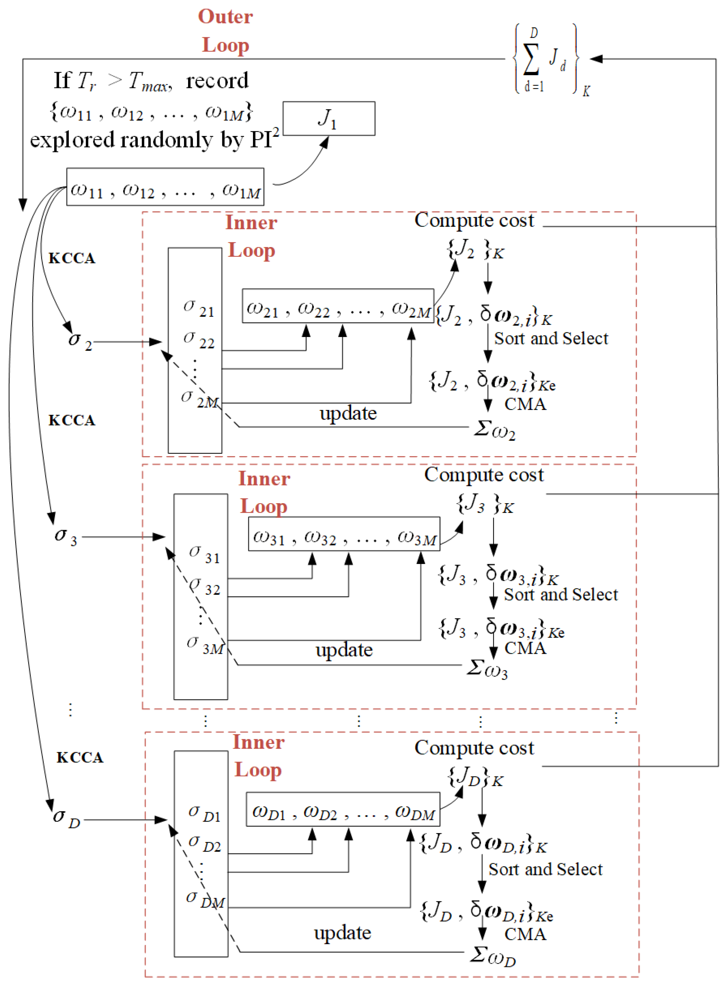
4. PI²-CMA with Kernel Canonical Correlation Analysis

In Equation (3), it can be seen that the perturbation $\mathbf{\epsilon }$ of PI² is generated with equal probability for each joint’s weight vector ${\mathbf{\omega }}_d$. The PI${}^2$-CMA takes into account the implicit linear correlations between the basis functions of the joint and automatically updates the covariance. However, when a task is assigned to a multi-joint robot, there exists an unknown hidden task-oriented pattern between weight vector with perturbation ${\check{\mathbf{\omega }}}_{d_i}$ and ${\check{\mathbf{\omega }}}_{d_j}$ (${\check{\mathbf{\omega }}}_{d_k}={\mathbf{\omega }}_{d_k}+\delta {\mathbf{\omega }}_{d_k},k\in \{i,j\}$). The pattern can be inferred from experience and expressed as a nonlinear correlation. Specifically, we can apply Kernel Canonical Correlation Analysis (KCCA) to infer the implicit nonlinear heuristic information between the joints of the robot to guide PI${}^2$ to a search policy for the new task of trajectory planning. In the paper, we not only consider the linear correlations between the perturbation vector’s components within a DMP but also take nonlinear correlations of the perturbation vector between DMPs into account to expedite the learning procedure of the robot.

4.1. Nonlinear Correlation Heuristic Information

According to Equations (3) and (4), perturbation is generated with equal probability for each joint’s weight vector. In other words, there is no correlation between the joints. Therefore, ${[{\check{\mathbf{\omega }}}_1^T,{\check{\mathbf{\omega }}}_2^T,\cdots ,{\check{\mathbf{\omega }}}_D^T]}^T\in {\mathbb{R}}^{DM\times 1}$ is denoted as $\tilde{\mathbf{\omega }}$, and covariance matrix of $\tilde{\mathbf{\omega }}$ is given by:

$${\mathsf{\Sigma }}_{\tilde{\mathbf{\omega }}}=diag[{\mathbf{\sigma }}_1^2,{\mathbf{\sigma }}_2^2,\cdots ,{\mathbf{\sigma }}_D^2]\in {\mathbb{R}}^{DM\times DM},$$

(8)

where $diag[·]$ represents diagonal matrix and ${\mathbf{\sigma }}_1^2=\cdots ={\mathbf{\sigma }}_D^2={\mathbf{\sigma }}^2$.

When the multi-joint robot completes the task, we believe that there are some hidden patterns between the joints. The implicit patterns between the perturbation vectors of the multi-joint robot are expressed as nonlinear correlations. With the help of the kernel method, the dth joint’s perturbation vector ${\check{\mathbf{\omega }}}_d\in {\mathbb{R}}^{M\times 1}$ is mapped to high-dimensional feature space $\varphi \left({\check{\mathbf{\omega }}}_d\right)\in {\mathbb{R}}^{V\times 1}$. $\tilde{\mathbf{\omega }}$ is also mapped to high-dimensional feature space $\varphi \left(\tilde{\mathbf{\omega }}\right)\in {\mathbb{R}}^{DV\times 1}$, and then covariance matrix of $\tilde{\mathbf{\omega }}$ can be described as:

$${\mathsf{\Sigma }}_{\varphi \left(\tilde{\mathbf{\omega }}\right)}=\left[\begin{array}{cccc}\Gamma ({\check{\mathbf{\omega }}}_1,{\check{\mathbf{\omega }}}_1)& \Gamma ({\check{\mathbf{\omega }}}_1,{\check{\mathbf{\omega }}}_2)& \cdots & \Gamma ({\check{\mathbf{\omega }}}_1,{\check{\mathbf{\omega }}}_D)\\ \Gamma ({\check{\mathbf{\omega }}}_2,{\check{\mathbf{\omega }}}_1)& \Gamma ({\check{\mathbf{\omega }}}_2,{\check{\mathbf{\omega }}}_2)& \cdots & \Gamma ({\check{\mathbf{\omega }}}_2,{\check{\mathbf{\omega }}}_D)\\ ⋮& ⋮& \ddots & ⋮\\ \Gamma ({\check{\mathbf{\omega }}}_D,{\check{\mathbf{\omega }}}_1)& \Gamma ({\check{\mathbf{\omega }}}_D,{\check{\mathbf{\omega }}}_2)& \cdots & \Gamma ({\check{\mathbf{\omega }}}_D,{\check{\mathbf{\omega }}}_D)\end{array}\right],$$

(9)

where $\Gamma ({\check{\mathbf{\omega }}}_{d_i},{\check{\mathbf{\omega }}}_{d_j})=cov(\varphi \left({\check{\mathbf{\omega }}}_{d_i}\right),\varphi \left({\check{\mathbf{\omega }}}_{d_j}\right))$ is the covariance of ${\check{\mathbf{\omega }}}_{d_i}$ and ${\check{\mathbf{\omega }}}_{d_j}$ projected on high-dimensional space, expressing the implicit nonlinear pattern between the perturbation vectors of the $d_i$th joint and the $d_j$th joint. The intuitive policy is to obtain ${\Sigma }_{\varphi \left(\tilde{\mathbf{\omega }}\right)}$ based on empirical samples, and then use $\Gamma ({\check{\mathbf{\omega }}}_{d_i},{\check{\mathbf{\omega }}}_{d_j})$ as the heuristic information. That is, given the perturbation vector ${\check{\mathbf{\omega }}}_{d_i}$, the exploration of ${\check{\mathbf{\omega }}}_{d_j}$ is guided by the covariance $\Gamma ({\check{\mathbf{\omega }}}_{d_i},{\check{\mathbf{\omega }}}_{d_j})$.

Note that $\Gamma ({\check{\mathbf{\omega }}}_{d_i},{\check{\mathbf{\omega }}}_{d_j})$ is in the unified space coordinate system (i.e., $\varphi \left(\check{\mathbf{\omega }}\right)$), but analyzing the correlation between the perturbation vector ${\check{\mathbf{\omega }}}_{d_i}$ of the $d_i$th joint and the perturbation vector ${\check{\mathbf{\omega }}}_{d_j}$ of the $d_j$th joint in a uniform coordinate system is not the best choice. Because after the perturbation vectors of different joints are mapped to a high-dimensional space, the correlation coefficients between the joints can be maximized only after a proper projection transformation, and such projection matrices are usually not necessarily identical. Here, the generalized Rayleigh Entropy is used to find the maximum correlation coefficient of $\varphi \left({\check{\mathbf{\omega }}}_{d_i}\right)$ and $\varphi \left({\check{\mathbf{\omega }}}_{d_j}\right)$, and Maximum Likelihood Estimation is used to infer the nonlinear correlation between ${\check{\mathbf{\omega }}}_{d_i}$ and ${\check{\mathbf{\omega }}}_{d_j}$. If $d_i\ne d_j$, $\Theta ({\check{\mathbf{\omega }}}_{d_i},{\check{\mathbf{\omega }}}_{d_j})=cov(P_r\left\{\Phi \left({\check{\mathbf{\omega }}}_{d_i}\right)\right\},P_r\left\{\Phi \left({\check{\mathbf{\omega }}}_{d_j}\right)\right\})$ can be the heuristic information, and $P_r$ is the projection operator. That is, given the perturbation vector ${\check{\mathbf{\omega }}}_{d_i}$, ${\check{\mathbf{\omega }}}_{d_j}$ can be obtained from the covariance $\Theta ({\check{\mathbf{\omega }}}_{d_i},{\check{\mathbf{\omega }}}_{d_j})$. Equation (9) can now be expressed as follows:

$${\mathsf{\Sigma }}_{\varphi \left(\tilde{\mathbf{\omega }}\right)}^{+}=\left[\begin{array}{cccc}\Gamma ({\check{\mathbf{\omega }}}_1,{\check{\mathbf{\omega }}}_1)& \Theta ({\check{\mathbf{\omega }}}_1,{\check{\mathbf{\omega }}}_2)& \cdots & \Theta ({\check{\mathbf{\omega }}}_1,{\check{\mathbf{\omega }}}_D)\\ \Theta ({\check{\mathbf{\omega }}}_2,{\check{\mathbf{\omega }}}_1)& \Gamma ({\check{\mathbf{\omega }}}_2,{\check{\mathbf{\omega }}}_2)& \cdots & \Theta ({\check{\mathbf{\omega }}}_2,{\check{\mathbf{\omega }}}_D)\\ ⋮& ⋮& \ddots & ⋮\\ \Theta ({\check{\mathbf{\omega }}}_D,{\check{\mathbf{\omega }}}_1)& \Theta ({\check{\mathbf{\omega }}}_D,{\check{\mathbf{\omega }}}_2)& \cdots & \Gamma ({\check{\mathbf{\omega }}}_D,{\check{\mathbf{\omega }}}_D)\end{array}\right].$$

(10)

4.2. Robot Intelligent Trajectory Inference with KCCA

KCCA [14] is a nonlinear correlation analysis method. In this paper, we employ KCCA on the elite samples from the robot’s first joint to other joints, and make heuristic inference. After the pth iteration of PI²-CMA, the program records the total reward $J^p\left(\tau \right)$ (one episodic samples), based on the current ${\check{\mathbf{\omega }}}_{1,\cdots ,D}^p$ (perturbation vectors of D joints). Then, $J^p\left(\tau \right)$ is compared with the total reward $J^{p-1}\left(\tau \right)$ based on ${\check{\mathbf{\omega }}}_{1,\cdots ,D}^{p-1}$ at the (p−1)th iteration to obtain a decline rate $T_r$.

If $T_r$ is greater than its upper threshold $T_{max}$, $T_r$ is updated to $T_{max}$, and the program executes KCCA learning. At this time, the weight perturbation sample ${\check{\mathbf{\omega }}}_1^s=\{{\check{\mathbf{\omega }}}_{1,1},{\check{\mathbf{\omega }}}_{1,2},\cdots ,{\check{\mathbf{\omega }}}_{1,N}\}$ on the first joint and the weight perturbation sample ${\check{\mathbf{\omega }}}_2^s=\{{\check{\mathbf{\omega }}}_{2,1},{\check{\mathbf{\omega }}}_{2,2},\cdots ,{\check{\mathbf{\omega }}}_{2,N}\}$ on the second joint in the pth iteration are respectively mapped in high dimensions to obtain $[\varphi \left({\check{\mathbf{\omega }}}_{d,1}\right)\varphi \left({\check{\mathbf{\omega }}}_{d,2}\right)\cdots \varphi \left({\check{\mathbf{\omega }}}_{d,N}\right)]$, denoted as $\Phi \left({\check{\mathbf{\omega }}}_d^s\right)\in {\mathbb{R}}^{V\times N}(d\in [1,2])$. Next, find two sets of vectors $w_1$, $w_2\in {\mathbb{R}}^{V\times 1}$, so that the correlation coefficient between the data u and v after the projection of $\varphi \left({\check{\mathbf{\omega }}}_1\right)$ and $\varphi \left({\check{\mathbf{\omega }}}_2\right)$ is maximized. We will have:

$$\begin{array}{c}\hfill u=w_1^T\varphi \left({\check{\mathbf{\omega }}}_1\right),\\ \hfill v=w_2^T\varphi \left({\check{\mathbf{\omega }}}_2\right).\end{array}$$

(11)

The covariance of u and v is given by:

$$var(u,v)=\frac{1}{N-1}{w}_1^T\Phi \left({\check{\mathbf{\omega }}}_1^s\right)\Phi {\left({\check{\mathbf{\omega }}}_2^s\right)}^T{w}_2.$$

(12)

Obviously, the vectors $w_1$ and $w_2$ are located in the space spanned by data $\Phi \left({\check{\mathbf{\omega }}}_1^s\right)$ and $\Phi \left({\check{\mathbf{\omega }}}_2^s\right)$:

$$\begin{array}{c}\hfill w_1=\Phi \left({\check{\mathbf{\omega }}}_1^s\right){\mathbf{\alpha }}_{\mathbf{1}},\\ \hfill w_2=\Phi \left({\check{\mathbf{\omega }}}_2^s\right){\mathbf{\alpha }}_{\mathbf{2}},\end{array}$$

(13)

where ${\mathbf{\alpha }}_1$, ${\mathbf{\alpha }}_2\in {\mathbb{R}}^{N\times 1}$. From Equations (12) and (13), correlation coefficient $\rho$ can be obtained:

$$\begin{array}{cc}\hfill \rho & =\frac{{\mathbf{\alpha }}_1^T{\Phi }^T\left({\check{\mathbf{\omega }}}_1^s\right)\Phi \left({\check{\mathbf{\omega }}}_1^s\right){\Phi }^T\left({\check{\mathbf{\omega }}}_2^s\right)\Phi \left({\check{\mathbf{\omega }}}_2^s\right){\mathbf{\alpha }}_2}{{\sqrt{{\mathbf{\alpha }}_1^T{\left({\Phi }^T\left({\check{\mathbf{\omega }}}_1^s\right)\Phi \left({\check{\mathbf{\omega }}}_1^s\right)\right)}^2\mathbf{\alpha }}}_1\sqrt{{\mathbf{\alpha }}_2^T{\left({\Phi }^T\left({\check{\mathbf{\omega }}}_2^s\right)\Phi \left({\check{\mathbf{\omega }}}_2^s\right)\right)}^2{\mathbf{\alpha }}_2}}\hfill \\ \hfill & =\frac{{\mathbf{\alpha }}_1^T{K}_{{\omega }_1}{K}_{{\omega }_2}{\mathbf{\alpha }}_2}{\sqrt{{\mathbf{\alpha }}_1^T{K}_{{\omega }_1}{K}_{{\omega }_1}{\mathbf{\alpha }}_1}\sqrt{{\mathbf{\alpha }}_2^T{K}_{{\omega }_2}{K}_{{\omega }_2}{\mathbf{\alpha }}_2}}.\hfill \end{array}$$

(14)

Kernel method is introduced in Equation (14), where $K(·)$ is a kernel matrix. Without loss of generality, we fixed the denominator ${\mathbf{\alpha }}_1^T{K}_{{\omega }_1}{K}_{{\omega }_1}{\mathbf{\alpha }}_1=1$, ${\mathbf{\alpha }}_2^T{K}_{{\omega }_2}{K}_{{\omega }_2}{\mathbf{\alpha }}_2=1$ of Equation (14) to find a suitable ${\mathbf{\alpha }}_1$ and ${\mathbf{\alpha }}_2$ to maximize ${\mathbf{\alpha }}_1^T{K}_{{\omega }_1}{K}_{{\omega }_2}{\mathbf{\alpha }}_2$. Construct the Lagrange function:

$$\begin{array}{cc}\hfill L=& {\mathbf{\alpha }}_1^T{K}_{{\omega }_1}{K}_{{\omega }_2}{\mathbf{\alpha }}_2-\frac{{\lambda }_1}{2}({\mathbf{\alpha }}_1^T{K}_{{\omega }_1}{K}_{{\omega }_1}{\mathbf{\alpha }}_1-1)\hfill \\ \hfill & -\frac{{\lambda }_2}{2}({\mathbf{\alpha }}_2^T{K}_{{\omega }_2}{K}_{{\omega }_2}{\mathbf{\alpha }}_2-1).\hfill \end{array}$$

(15)

We take partial derivatives of ${\alpha }_1$ and ${\alpha }_2$ in Equation (15), and obtain:

$$\left\{\begin{array}{c}{K}_{{\omega }_2}{\mathbf{\alpha }}_2=\lambda K_{{\omega }_1}{\mathbf{\alpha }}_1\hfill \\ \lambda =2{\lambda }_1=2{\lambda }_2={\mathbf{\alpha }}_1^T{K}_{{\omega }_1}{K}_{{\omega }_2}{\mathbf{\alpha }}_2.\hfill \end{array}\right.$$

(16)

According to Equation (16), the implicit correlation P${}_{ca}$$\left(\mathsf{\Theta }({\check{\mathbf{\omega }}}_1,{\check{\mathbf{\omega }}}_2)\right)$ between the first joint and the second joint perturbation vector of the robot is obtained. When the current $T_r$ is greater than the upper threshold $T_{max}$, ${\mathbf{\alpha }}_1,{\mathbf{\alpha }}_2$ are recorded. Furthermore, Equation (15) can be repeatedly executed to obtain the implicit correlation between the first joint and the dth ($d\in [2,\cdots ,D]$) joint. In this way, we get the implicit patterns $\{({\mathbf{\alpha }}_1,{\mathbf{\alpha }}_2),\cdots ,({\mathbf{\alpha }}_1,{\mathbf{\alpha }}_D)\}$ between the joints.

If $T_r$ is less than the lower threshold $T_{min}$, the independent explorations of the whole joint are abandoned, and the KCCA prediction is turned on. That is, the first joint explores randomly to obtain a perturbation sample ${\check{\mathbf{\omega }}}_1^s$ and $K_{{\omega }_1}$ in the pth iteration, then (${\mathbf{\alpha }}_1,{\mathbf{\alpha }}_2$) is used to calculate $K_{{\omega }_2}$ of the second joint. Obviously, ${\check{\mathbf{\omega }}}_2$ can be computed from $K_{{\omega }_2}$, and that will guide the exploration of the second joint. Repeat the same steps for the subsequent joints until the Dth joint.

4.3. The Combination of KCCA and CMA

We draw the schematic of the PI²-CMA-KCCA’s control flow as Figure 1, which works like a double closed-loop control system. Without loss of generality, there are D joints, and each joint corresponds to M basis functions, then $D\times M$ parameters need to be adjusted.

The outer loop aims at discovering the hidden patterns between the joints which are helpful to fulfill the new task. Specifically, we use the KCCA to infer the nonlinear correlations between the first joint and other joints for good declining rate, recorded as $\{({\mathbf{\alpha }}_1,{\mathbf{\alpha }}_2),\cdots ,({\mathbf{\alpha }}_1,{\mathbf{\alpha }}_D)\}$. After that, we can compute ${\check{\mathbf{\omega }}}_d$ from $K_{{\omega }_d}$ based on perturbation sample ${\check{\mathbf{\omega }}}_1^s$ and $K_{{\omega }_1}$, and it will guide the perturbation of the dth joint as a means of exploring noise.

The inner loop extracts heuristic information from a corresponding single joint to guide the search. Specifically, in the previous iteration, it evaluates the cost $J_d$ of K roll-outs (sorting and probability average), then selects the first $K_e$ elites of the perturbation sample to obtain the covariance ${\Sigma }_{{\mathbf{\omega }}_d}$ by the CMA algorithm. Furthermore, in current iteration, ${\mathbf{\omega }}_d\sim \mathcal{N}\left({\check{\mathbf{\omega }}}_d,{\Sigma }_{{\mathbf{\omega }}_d}\right)$ is used to explore the policy parameter ${\mathbf{\omega }}_d$. In other words, it applies compound heuristic information which integrates the inferred hidden nonlinear patterns between the joints and the linear patterns within the joint to automatically determine the exploring proportion for each component of ${\mathbf{\omega }}_d$.

In short, the outer loop discovers and predicts the exploring mean of ${\mathbf{\omega }}_d$ for the dth ($d\ne 1$) DOF, the inner loop discloses and infers the exploring variance of ${\mathbf{\omega }}_d$ for the dth ($d\ne 1$) DOF. As for 1st DOF, a vanilla PI${}^2$ is employed.

5. Evaluations

The cost function in our experiments is given by:

$$\begin{array}{cc}\hfill J=& 0.5\times \sum _{d=1}^D\sum _{i=1}^{N-1}[{10}^7{\left({\ddot{y}}^{\left(d\right)}\left(i\right)\right)}^2+{\left(a_f^{\left(d\right)}\left(i\right)\right)}^2]\hfill \\ \hfill & +\sum _{d=1}^D{10}^{11}{(y^{\left(d\right)}\left(m\right)-y_v^{\left(d\right)})}^2\hfill \\ \hfill & +\sum _{d=1}^D{10}^3[{\left({\dot{y}}^{\left(d\right)}\right)}^2+{(y^{\left(d\right)}\left(N\right)-y_g^{\left(d\right)})}^2].\hfill \end{array}$$

(17)

In Equation (17), D is the number of joints of SCARA and Swayer. $y^{\left(d\right)}\left(i\right),{\dot{y}}^{\left(d\right)}\left(i\right),{\ddot{y}}^{\left(d\right)}\left(i\right)$ denote the position, velocity, and acceleration of the dth joint of the robot at the time i. $y_v^{\left(d\right)}$ is the present point (i.e., via-point) to be passed through by the dth joint at time i. $y_g^{\left(d\right)}$ is the trajectory’s end point of the d joint. $y^d\left(m\right)$ is the point passed through by the dth joint at time m. $a_f^{\left(d\right)}\left(i\right)$ is the acceleration of forcing term of the dth joint at time i. Equation (17) is a typical quadratic expression of total reward in the finite stage of reinforcement learning.

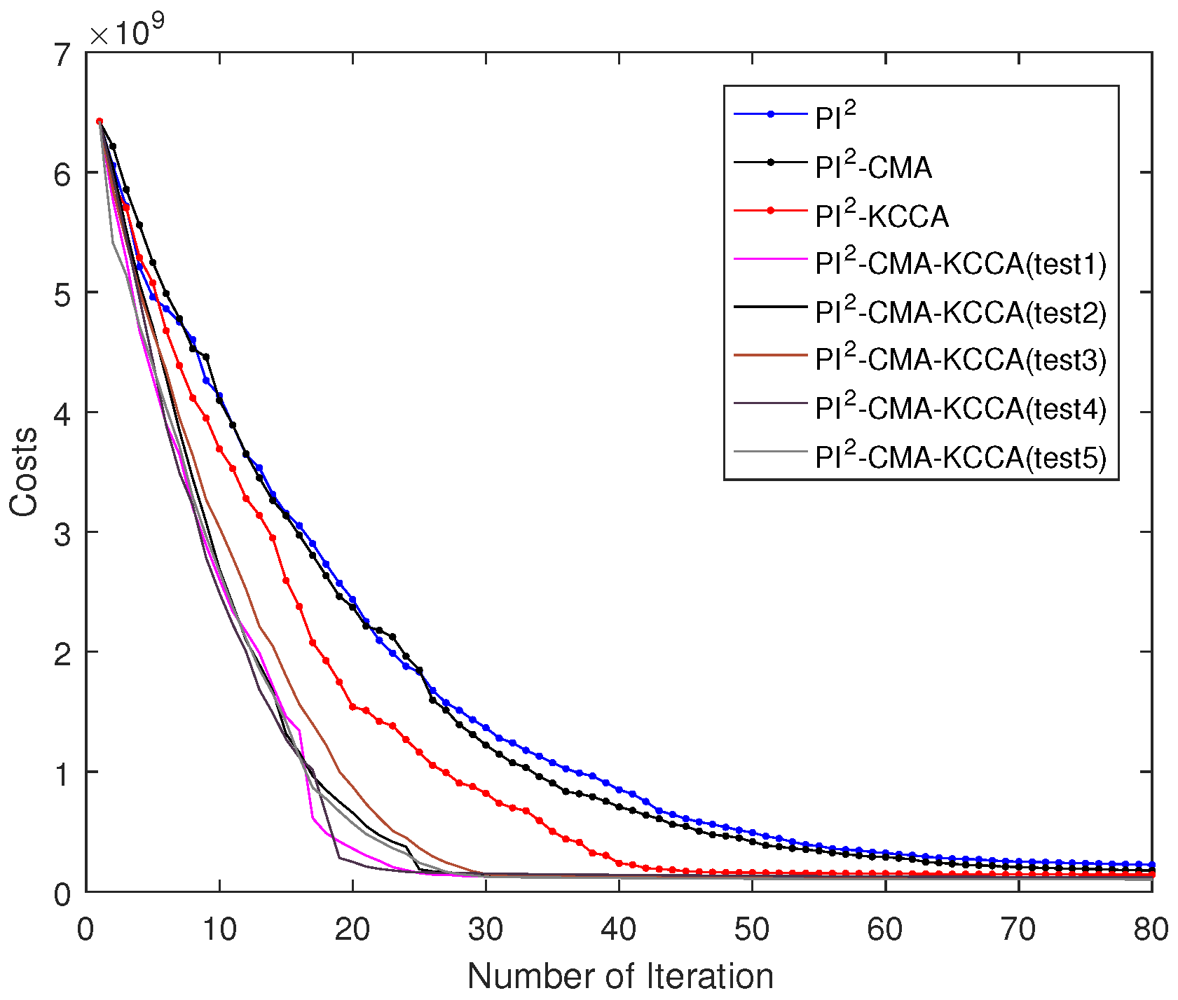
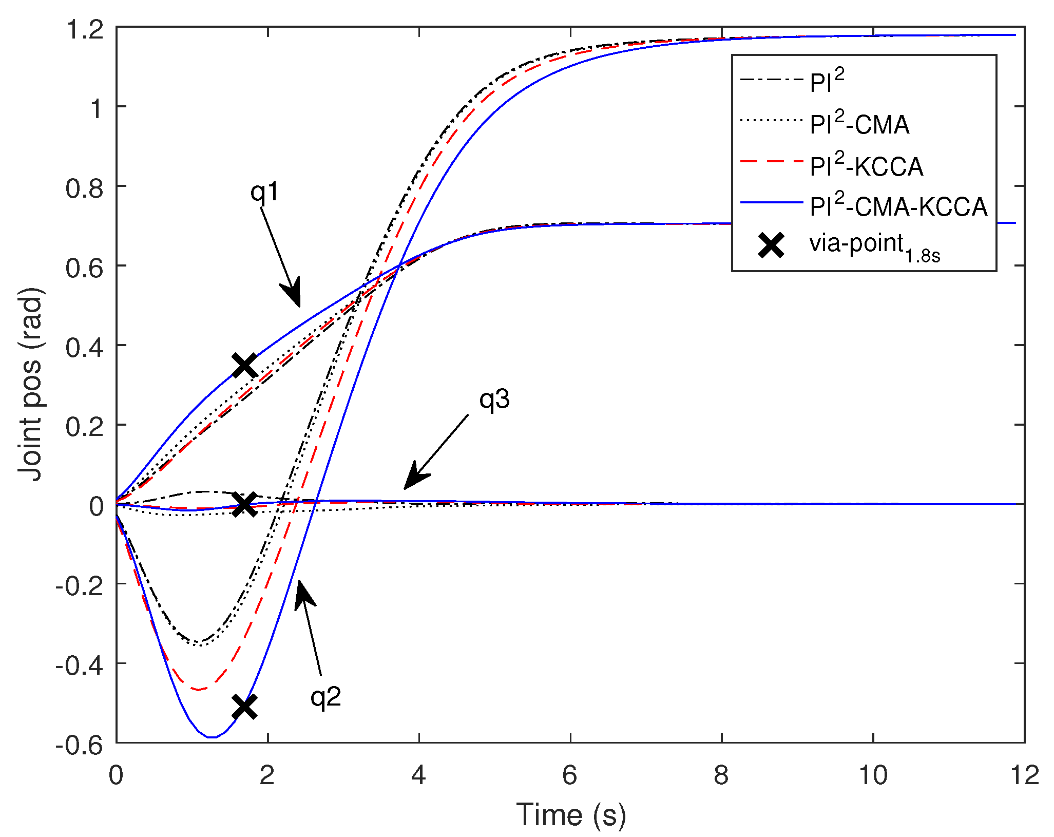
5.1. Passing through One Via-Point with SCARA

SCARA has three revolute joints $q_1$, $q_2$, $q_3$ and one prismatic joint $q_4$. In this experiment, the orientation of the end-effector of the robot arm is ignored, thus the SCARA robot arm can be regarded as a planar two-link mechanism.

The experiment is divided into the following four steps: $\left(\mathbf{1}\right)$ Set the Cartesian coordinate of the starting position of the end-effector to ${(20,0,0)}^{\mathrm{T}}$cm, and the corresponding joint angle is ${(0,0,0)}^{\mathrm{T}}$rad. Set the endpoint ${(4.5,16,0)}^{\mathrm{T}}$cm, and the corresponding joint angle is ${(0.7068,1.1796,0)}^{\mathrm{T}}$rad. $\left(\mathbf{2}\right)$ Drive the manipulator based on the principle of minimum jitter to obtain the demonstration. $\left(\mathbf{3}\right)$ Given a new task, use PI², PI²-CMA, PI²-KCCA, and PI²-CMA-KCCA, respectively, to make the movement pass through a via-point at $m=1.8 \mathrm{s}$. $\left(\mathbf{4}\right)$ The four algorithms are iterated for 80 times respectively to gain new motor skills.

In this experiment, each of the four different algorithms is repeated 20 times. The best experimental results of PI², PI²-CMA, PI²-KCCA, and the five experimental results of PI²-CMA-KCCA are selected for comparison. The optimization effect of PI²-CMA-KCCA is analyzed by comparing the final cost of the system and the trajectories of joint space. It can be clearly seen from Figure 2 that PI²-CMA-KCCA converges faster, and its final cost is the lowest (as shown in

Table 2. The final cost of one via-point task with SCARA.

Algorithm	Final Cost
PI2	$2.2341\times {10}^8$
PI2-CMA	$1.7569\times {10}^8$
PI2-KCCA	$1.4089\times {10}^8$
PI2-CMA-KCCA(test1)	$1.0249\times {10}^8$
PI2-CMA-KCCA(test2)	$1.1095\times {10}^8$
PI2-CMA-KCCA(test3)	$1.0677\times {10}^8$
PI2-CMA-KCCA(test4)	$1.2106\times {10}^8$
PI2-CMA-KCCA(test5)	$1.0155\times {10}^8$

).

Figure 3 shows the movement trajectories of the three joints of the SCARA in the joint space when the number of iterations is 35. Because the joint $q_3$ has no effect on the position of the end-effector, the value of $q_3$ in the joint space remains constant.

The blue line in Figure 3 is the trajectory of each joint of the robot arm under the PI²-CMA-KCCA. Figure 3 demonstrates that only the blue lines pass through an intermediate via-point.

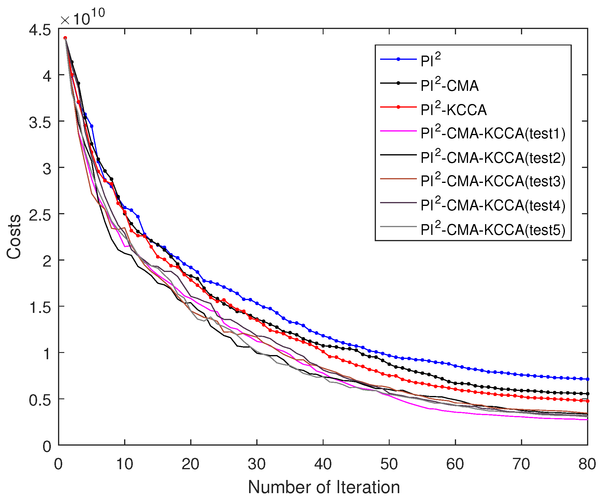
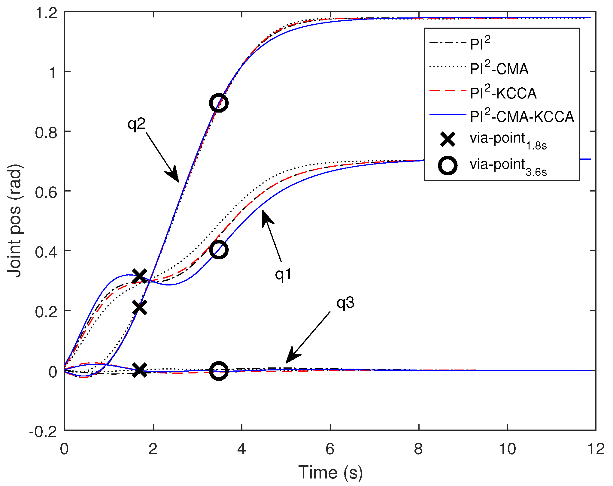
5.2. Passing through Two Via-Point with SCARA

This experimental procedure is similar to Section 5.1, requiring the end-effector to pass the point ${(18.2,8.1,0)}^{\mathrm{T}}$ cm at $m=1.8$ s and the point ${(12.0,13.5,0)}^{\mathrm{T}}$ cm at $m=3.6$ s. Four different algorithms are also respectively repeated 20 times, and the best experimental results of PI², PI²-CMA, PI²-KCCA, and the five experimental results of PI²-CMA-KCCA are selected for comparison. Figure 4 demonstrates that the PI²-CMA-KCCA has better learning performance than the other algorithms. After 80 iterations, the final cost of the four algorithms is given in

Table 3. The final cost of two via-point task with SCARA.

Algorithm	Final Cost
PI2	$7.1203\times {10}^9$
PI2-CMA	$5.5471\times {10}^9$
PI2-KCCA	$4.4999\times {10}^9$
PI2-CMA-KCCA(test1)	$2.7410\times {10}^9$
PI2-CMA-KCCA(test2)	$3.3489\times {10}^9$
PI2-CMA-KCCA(test3)	$3.4429\times {10}^9$
PI2-CMA-KCCA(test4)	$3.1620\times {10}^9$
PI2-CMA-KCCA(test5)	$3.0731\times {10}^9$

.

Figure 5 shows the trajectories of the three joints of the SCARA in the joint space when the number of iterations is 50, where the blue lines represent the joints’ trajectories of the robot arm in joint space under the PI²-CMA-KCCA. It demonstrates that, when the number of iterations is 50, the blue trajectories pass through two intermediate via-point at $t=1.8$ s and $t=3.6$ s accurately.

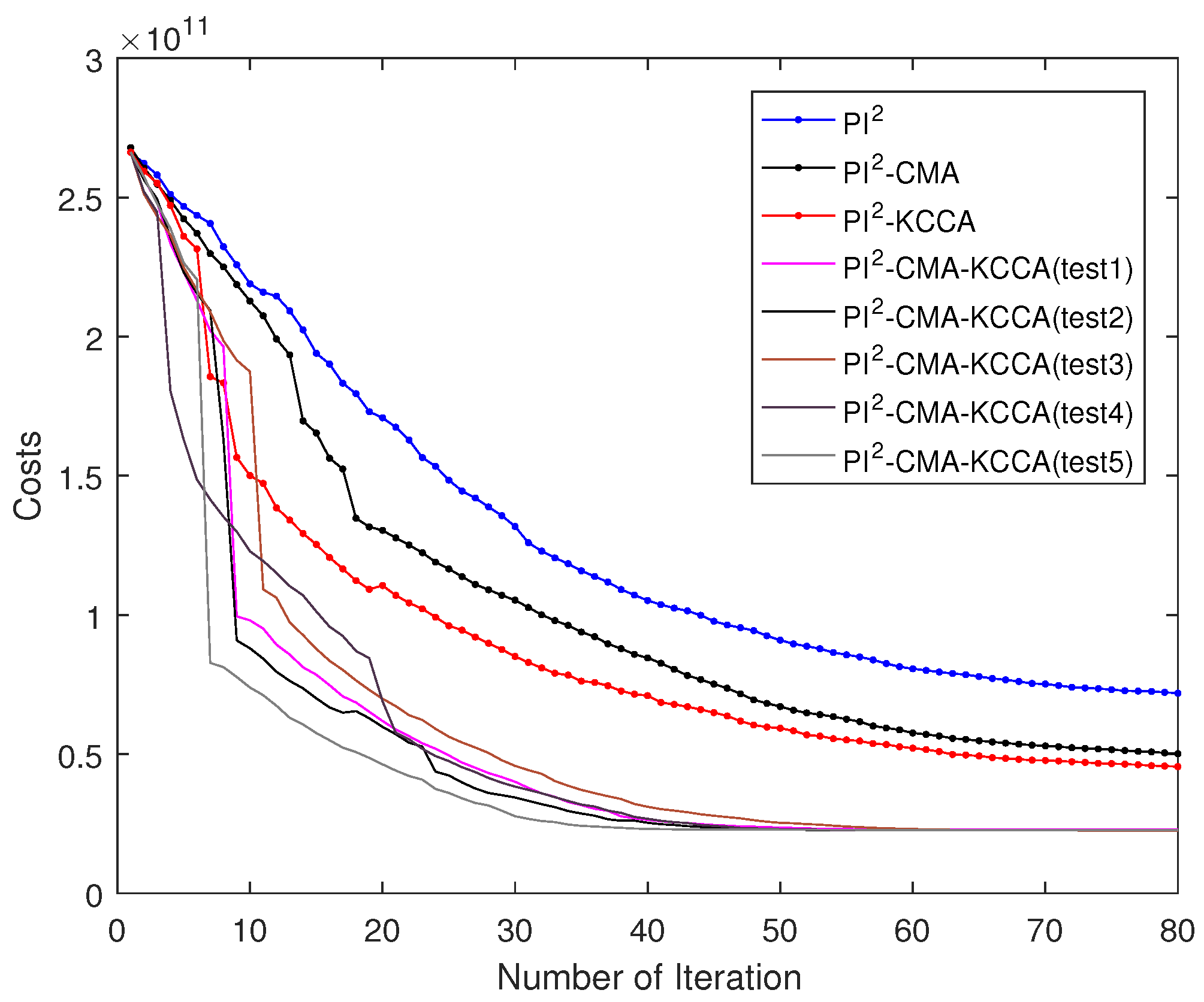
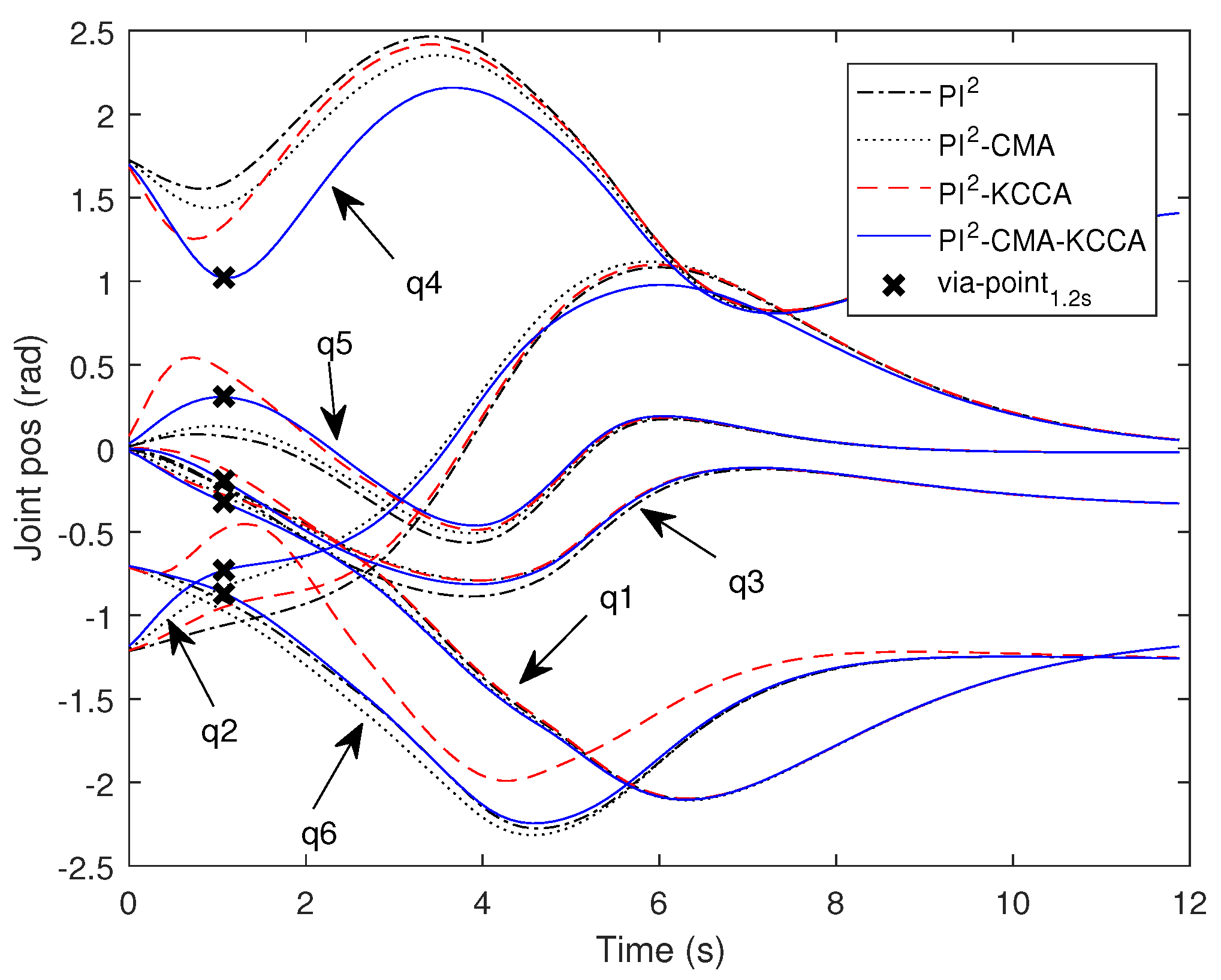
5.3. Passing Through One Via-Point with Swayer

Swayer is a lightweight collaborative robot created by Rethink Robotics. It has seven joints. In this subsection, $q_i$ is used to represent the ith joint of Swayer. Because the $q_7$ has no effect on Cartesian position of the end-effector, only six joints are considered. This experiment uses the ROS platform to control the movement trajectory of the Swayer manipulator in the Ubuntu16 system, and validates the effectiveness of the PI²-CMA-KCCA.

First, we set an arbitrary starting point ${(697,159,514)}^{\mathrm{T}}$ mm in the workspace of Swayer and an arbitrary endpoint ${(300,-569,-65)}^{\mathrm{T}}$ mm, then drag Swayer to record a demonstration from the starting point to the endpoint, then choose any reachable point ${(840,-248,595)}^{\mathrm{T}}$ mm far away from the demonstration as a new task at $m=1.2$ s. Finally, PI², PI²-CMA, PI²-KCCA, and PI²-CMA-KCCA are repeated 20 times on Swayer. The five experimental results of the PI²-CMA-KCCA and the best experimental results of the PI², PI²-CMA and PI²-KCCA are selected for analysis. Figure 6 shows the downward trend of the cost of the four algorithms, and the final cost of the four algorithms after 80 iterations is given in

Table 4. The final cost of one via-point task with Swayer.

Algorithm	Final Cost
PI2	$7.1889\times {10}^{10}$
PI2-CMA	$5.0168\times {10}^{10}$
PI2-KCCA	$4.5494\times {10}^{10}$
PI2-CMA-KCCA(test1)	$2.2861\times {10}^{10}$
PI2-CMA-KCCA(test2)	$2.2581\times {10}^{10}$
PI2-CMA-KCCA(test3)	$2.2641\times {10}^{10}$
PI2-CMA-KCCA(test4)	$2.2554\times {10}^{10}$
PI2-CMA-KCCA(test5)	$2.2513\times {10}^{10}$

.

Figure 6 illustrates that during the reinforcement learning, learning efficiency of PI²-CMA-KCCA is higher under the same number of iterations. At the same time, Figure 7 shows that the Swayer passes through an intermediate via-point accurately at $m=1.2$ s when the number of iterations is 60.

Figure 7 shows the trajectories of joint space in Swayer. The blue lines represent the joints’ trajectories after PI²-CMA-KCCA learning. The result shows that only the blue lines can pass through the via-point accurately after about 60 iterations.

5.4. Performance Comparison of Four Algorithms

In

Table 5. Average decline rate of four algorithms.

Task	PI2	PI2-CMA	PI2-KCCA	PI2-CMA-KCCA
One Via-Point Task with SCARA	96.5%	97.2%	97.8%	98.5%
Two Via-Point Task with SCARA	84.0%	87.4%	89.7%	92.8%
One Via-Point Task with Swayer	73.0%	81.3%	83.0%	91.5%

, the cost decline rate of PI²-CMA-KCCA is always higher than that of PI², PI²-CMA, and PI²-KCCA. When the experimental objects are the same, the new task is more complicated, and the learning performance of PI²-CMA-KCCA is better than that of the other three algorithms. In addition, especially when the tasks are the same, the greater the number of degrees of freedom of the experimental objects, the better the optimization effect of PI²-CMA-KCCA than the other algorithms because PI²-CMA-KCCA not only adjusts the magnitude of exploration noise automatically but also considers the nonlinear heuristic information between the joints.

6. Conclusions

Compound heuristic information is applied in the paper to guide PI2’s variational exploration and expedite the procedure of reinforcement learning. This information is derived by KCCA and CMA together. KCCA infers the nonlinear heuristic information between the joints of robot, and CMA infers the linear heuristic information within single DOF. This information may cause the cost function to drop rapidly with the MLE on the roll-out data. In addition, the proposed algorithm PI²-CMA-KCCA works like a double closed-loop control system, in which the outer loop discovers and predicts the means of exploring vectors for each DOF and the inner loop discloses and infers the variance of exploring vector for each DOF. In this way, the new algorithm can quickly search the optimal parameters of new tasks. The experimental results on SCARA and Swayer also demonstrate that the algorithm can speed up the process of updating parameters while maintaining the accuracy of completing new tasks, which is suitable for multi-degree-of-freedom objects and more complex tasks.

References

1. Siciliano, B.; Khatib, O. Springer Handbook of Robotics; Springer: Berlin/Heidelberg, Germany, 2016; pp. 987–1008. [Google Scholar]
2. Takano, W.; Nakamura, Y. Statistical mutual conversion between whole body motion primitives and linguistic sentences for human motions. Int. J. Robot. Res. 2015, 34, 1314–1328. [Google Scholar]
3. Paraschos, A.; Daniel, C.; Peters, J.; Neumann, G. Probabilistic movement primitives. In Proceedings of the 27th Annual Conference on Neural Information Processing Systems, Lake Tahoe, NV, USA, 5–10 December 2013; pp. 2616–2624. [Google Scholar]
4. Khansari-Zadeh, S.M.; Billard, A. BM: An iterative algorithm to learn stable nonlinear dynamical systems with Gaussian mixture models. In Proceedings of the 2010 IEEE International Conference on Robotics and Automation, Anchorage, AK, USA, 3–7 May 2010; pp. 2381–2388. [Google Scholar]
5. Ratliff, N.D.; Bagnell, J.A.; Zinkevich, M.A. Maximum margin planning. In Proceedings of the 23rd International Conference on Machine Learning, Pittsburgh, PA, USA, 25–29 June 2006; pp. 729–736. [Google Scholar]
6. Sutton, R.S.; Barto, A.G. Reinforcement Learning; A Bradford Book; The MIT Press: Cambridge, MA, USA; London, UK, 1998; pp. 665–685. [Google Scholar]
7. Peters, J.; Schaal, S. Natural Actor-Critic. Neurocomputing 2008, 71, 1180–1190. [Google Scholar]
8. Kober, J.; Peters, J. Learning motor primitives for robotics. In Proceedings of the 2009 IEEE International Conference on Robotics and Automation, Kobe, Japan, 12–17 May 2009; pp. 2112–2118. [Google Scholar]
9. Peters, J.; Altun, Y. Relative entropy policy search. In Proceedings of the Twenty-Fourth AAAI Conference on Artificial Intelligence, Atlanta, GA, USA, 11–15 July 2010; pp. 1607–1612. [Google Scholar]
10. Theodorou, E.; Buchli, J.; Schaal, S. A Generalized Path Integral Control Approach to Reinforcement Learning. J. Mach. Learn. Res. 2010, 11, 3137–3181. [Google Scholar]
11. Stulp, F.; Sigaud, O. Path integral policy improvement with covariance matrix adaptation. In Proceedings of the 29 th International Conference on Machine Learning, Edinburgh, UK, 26 June–1 July 2012; pp. 281–288. [Google Scholar]
12. Fu, J.; Teng, X.; Cao, C.; Lou, P. Intelligent trajectory planning based on reinforcement learning with KCCA inference for robot. J. Huazhong Univ. Sci. Technol. (Nat. Sci. Ed.) 2019, 47, 96–102. [Google Scholar]
13. Ijspeert, A.J.; Nakanishi, J.; Hoffmann, H.; Pastor, P.; Schaal, S. Dynamical Movement Primitives: Learning Attractor Models for Motor Behaviors. Neural Comput. 2013, 25, 328–373. [Google Scholar]
14. Melzer, T.; Reiter, M.; Bischof, H. Appearance models based on kernel canonical correlation analysis. Pattern Recognit. 2003, 36, 1961–1971. [Google Scholar]
Figure 1. A typical system’s architecture for PI 2 -CMA-KCCA.
Applsci 10 05346 g001
Figure 2. Cost of one via-point task.
Applsci 10 05346 g002
Figure 3. One via-point task when the number of iterations is 30.
Applsci 10 05346 g003
Figure 4. Cost of two via-point task.
Applsci 10 05346 g004
Figure 5. Two via-point task when the number of iterations is 50.
Applsci 10 05346 g005
Figure 6. Cost of one via-point task.
Applsci 10 05346 g006
Figure 7. One via-point task when the number of iterations is 60.
Applsci 10 05346 g007