Investigation the Integration of Heliostat Solar Receiver to Gas and Combined Cycles by Energy, Exergy, and Economic Point of Views

Abstract

Due to the high amount of natural gas resources in Iran, the gas cycle as one of the main important power production system is used to produce electricity. The gas cycle has some disadvantages such as power consumption of air compressors, which is a major part of gas turbine electrical production and a considerable reduction in electrical power production by increasing the environment temperature due to a reduction in air density and constant volumetric airflow through a gas cycle. To overcome these weaknesses, several methods are applied such as cooling the inlet air of the system by different methods and integration heat recovery steam generator (HRSG) with the gas cycle. In this paper, using a heliostat solar receiver (HSR) in gas and combined cycles are investigated by energy, exergy, and economic analyses in Tehran city. The heliostat solar receiver is used to heat the pressurized exhaust air from the air compressor in gas and combined cycles. The key parameter of the three mentioned analyses was calculated and compared by writing computer code in MATLAB software. Results showed the use of HSR in gas and combined cycles increase the annual average energy efficiency from 28.4% and 48.5% to 44% and 76.5%, respectively. Additionally, for exergy efficiency, these increases are from 29.2% and 49.8% to 45.2% and 78.5%, respectively. However, from an economic point of view, adding the HRSG increases the payback period (PP) and it decreases the net present value (NPV) and internal rate of return (IRR).

1. Introduction

Iran’s total power generation capacity by thermal power plant stands at 66,000 MW (80%) in 2020, of which 37.8% are related to a gas turbine plant and 38.4% relate to combined power plants. So, the role of the gas turbine power plant is very substantial individually and in the combined power plants [1,2,3]. The performance of the gas turbine is affected by some important parameters that consist of the compression ratio, ambient temperature, and pressure, humidity, turbine inlet temperature, specific fuel consumption, and air to fuel ratio [4,5,6]. Due to the widespread use of gas power plants, it is important to consider the impact of these parameters on the efficiency of the gas turbines. Since the air of the combustion process in the gas turbine is provided by atmospheric air, so the specific properties of the atmospheric air in that reign is highly important. As the ambient temperature is one of the thermodynamic parameters, this factor has been studied extensively. Additionally, as the process of the gas turbine is the constant volume process, the investigation of this factor is being more highlighted [7,8]. The output power of gas turbine changes by an average of 10% since ambient temperature (compressor intake air) changes by 10 °C [9,10,11]. So, the performance of the gas turbine can be deteriorated significantly in the hot region or the summer season. On the other hand, the two operational considerations of the gas turbine are extensive regarding the application of the gas turbine. Firstly, a large amount of the output power of the turbine is required to drive the compressor (30–40%) in the gas power plant [12]. Secondly, the exhaust gas in the open gas power plant is quite high over 500 °C [7,13]. This excess heat in flue gas from the gas turbine can be used as a source of high-temperature resources in another cycle, unless it may cause thermal pollution of the atmosphere. The remedy for this high-temperature exhaust gas in the open gas cycle is neither to add bottoming steam cycle (combined cycle) [7,13] or using a heat recovery steam generator (HRSG) [14,15], as well as a combination of the solid oxide fuel cell and gas cycle.

The application of HRSG on the performance of gas turbines was examined for a steam power plant in Iran. The results revealed that adding an HRSG to a gas turbine, model Mitsubishi-701G2, could increase the energy and exergy efficiencies and power generation up to 52.19%, 50.9%, and 485.8 MW, respectively [16]. A general overview of different types of turbine air cooling methods in the gas power plants was examined. The three different air cooling methods consist of evaporative cooling, refrigeration cooling, and evaporative cooling of precompressed air that were introduced and examined [17]. The performance of three turbine air cooling methods applications including; evaporative media (EM), mechanical chiller (MC), and a novel idea of turbo-expander (TE) were conducted in the gas turbine of a refinery in Iran. The result showed that the efficiency improvement in the gas turbine cycle was 5% for mechanical chiller, 3% for evaporative media, and 4% for turbo-expander systems [18]. Najjar et al. [19] analyzed the effects of different methods of inlet air cooling systems for the gas turbine cycle. The results showed that evaporative cooling boosted power by up to 8.7% and efficiency by up to 3.3%. On the other hand, the fogging system improved power by up to 9.5% and efficiency by up to 3.5%. Moreover, the mechanical chiller reduced the temperature by 20–45 °C; enhancing the net power by 7–24.3% and improving the efficiency by 2.4–18.8%, whereas the absorption chillers enhanced the net power by up to 12.1–37.3% and improved the efficiency by up to 31.5%.

The performance usage of absorption chiller with lithium-bromide absorbent on the cooling of intake air of a gas turbine, operated either as a simple cycle or a combined cycle was examined in the arid and tropical climates (Thailand). Moreover, a feasibility study on the application of the waste heat from the exhaust gas of the gas cycles by using a heat recovery steam generator (HRSG) was studied. The results of this study showed, by taking the weather data of Bangkok (Thailand) that reduction of the ambient temperature to 15 °C could help to increase the rapid output power between 8 and 13%. The outcome of these output power changes led to 11% additional electricity generated from the same gas turbine power plant [20]. Wang et al. [21] were simulated the application of steam injection gas turbine (STIG) and inlet air cooling (IAC) system on the performance of the gas cycle. The obtained result revealed that both steam injection gas turbine (STIG) and inlet air cooling (IAC) systems increased more than 70% in output power and 20.4% improvement in heat rate. An extensive overview of the various combustion turbine inlet cooling technology (CTIAC) and the advantages and disadvantages concerning the environmental conditions and operational requirements were performed [22]. The application of adding a solar system to the gas turbine with and without storage systems is introduced as new technologies to the gas turbine power plant. In this technology, a solar system is used to heat up the compressed air in a gas turbine before entering the combustion chamber at certain levels. In this way, the air gets hotter, consequently, the mixture of air and fuel in the combustion chamber needs less fuel for the combustion process and this heat is compensated by solar energy. Schwarzböz et al. [23] conducted a study to compare solar gas turbine systems with other solar-fossil hybrid power plants. Moreover, in this study different scenarios were proposed to heat the pressurized air by application of a solar tower. The results revealed the annual average of the ration of solar to net electric efficiency was up 19%, amongst the highest conversion efficiencies for solar electric technologies. In addition, the economic analysis showed total plant investment costs from 7000 down to below 1800 €/kW, depending on power level and solar shares.

The description of the prototype solar-powered gas turbine system, installed during 2002 in Spain was reported by Heller et al. [24]. The results revealed that the 165 kW (115 kW solar contribution) electrical power was significantly lower than possible due to the reduced turbine speed and high ambient temperatures. The results revealed that the 165 kW (115 kW solar contribution) electrical power was significantly lower than possible due to the reduced turbine speed and high ambient temperatures. The application of different scenarios for solar gas turbine systems with different power levels was conducted. In this technology, a solar dish applied to heat up the pressurized air in a gas turbine before entering the combustion chamber at certain levels. Therefore, the share of fossil fuel in the combustion chamber was reduced and compensated by solar energy. By this action, the share of annual solar energy increased up to 30%. However, by applying solar systems with modern gas turbine systems led to increasing efficiencies of the solar heat from around 40% up to more than 50% [23]. A concentrated solar power (CSP) plant individually can be integrated with a natural gas-fired combined cycle (NGCC) power plant to produce excess steam consequently to generate more electricity. In other applications, the concentrated solar power (CSP) plant is applied to heat the compressed air in the gas turbine before entering the combustion chamber [25]. Alqahtani et al. [26] examined the performance of a hybrid integrated solar combined cycle (ISCCs). This hybrid system consisted of concentrated solar power (CSP) and a natural gas-fired combined cycle (NGCC) power plant. Results showed that this hybrid system could save 10–15% of nominal capacity from solar energy can be cost-effective as a dispatchable electricity generation resource. Moreover, the current levelized cost of electricity generation (LCOE) of an ISCC was lower than that of a gas-fired combined cycle (NGCC), when fuel price reached 13.5 $/MMBtu. Similar studies were carried out to evaluate the performance of a hybrid integrated solar combined cycle (ISCCs) [16,27,28].

Due to the reduction of the energy efficiency of gas and combined cycles caused by high ambient temperature, resolving this problem is essential especially in countries such as Iran. Moreover, Iran has a very high potential for solar energy utilization and the average sunshine in Iran is about 2800 hours per year [29]. Using a heliostat solar receiver (HSR) to increase the efficiency of the gas and combined cycle, which carried out in this research is very crucial and has not been performed in any previous research. So, application HSR can be used to preheat the air before entering the combustion chamber to reduce fuel consumption and efficiency improvement. In this regard, using an HSR system in the gas cycle (GC) and combined cycle (CC; the combination of gas turbine cycle integrated by heat recovery steam generator (HRSG)) is investigated by energy, exergy, and economic analyses. To achieve this target, GC and CC are modeled with/without an HSR system to reveal the benefit of this application. So, the quantify application of HSR in GC and CC cycles are one of the novelties of this research. In this regard, several important parameters such as energy and exergy efficiencies, net present value (NPV), payback period (PP), simple payback period (SPP), and internal rate of return (IRR) are calculated and compared to answer this question that using HSR systems is beneficial or not from energy, exergy, and economic point of views.

In summary, the innovation of this paper is as follows:

• Investigation of the integration of HSR via energy, exergy, and economic point of views;
• Calculation of the energy and exergy efficiencies of gas and combined cycles with and without HSR;
• Calculation of the economic key parameters such as NPV, IRR, PP, and SPP.

2. Mathematical Modeling

2.1. Process Description

In Figure 1a, a layout diagram of two cycles named gas cycle (GC) and steam cycle (SC) and integration (combined cycle (CC)) were demonstrated. In Figure 1b, the integration of this CC with the heliostat solar receiver (HSR) cycle is presented. The natural gas-based combined GC and heat recovery steam generator (HRSG) system is illustrated in Figure 1a. Additionally, Figure 1b depicts the combined gas turbine (GT)-HRSG-HSR system that employs solar energy by a heliostat solar receiver alongside natural gas to provide the thermal energy requirement of the plant. Both configurations are designed for power production using a gas turbine and a steam turbine. In the GT-HRSG combined system, Figure 1a, natural gas as fuel is sent to a combustion chamber (stream No. 11) by a booster compressor (BC), and air enters the combustion chamber (stream No. 2) from a compressor (C). The combustion chamber output goes to a gas turbine (stream No. 3) for power production. The flue gas of the gas turbine enters an HRSG unit (stream No. 4) to provide heat for a Rankine cycle (RC). The superheated steam leaves the HRSG unit to the turbine (T; stream No. 7) for more power production. The output fluid of the steam turbine is sent to a condenser (stream No. 8), and then is pumped back to the HRSG unit (stream No. 6).

In the integrated GT-HRSG-HSR configuration, Figure 1b, part of the heat energy demand is provided by the HSR. In HSR, Therminol VP-1 absorbs the heat reflected by the heliostat field as the working fluid and enters a storage tank (stream No. 3). The working fluid after heat exchange with exhaust pressurized air from the air compressor (stream No. 5) enters a pump (stream No. 1) to be pumped back to the receiver (stream No. 2). The hot air goes to a combustion chamber (stream No. 6), which includes natural gas as the fuel enters (stream No. 15). The combustion chamber output fluid enters a gas turbine (stream No. 7) for power production. The outlet stream goes to an HRSG unit to provide heat for the RC (stream No. 8). The steam of RC after gaining heat leaves the HRSG unit as superheated steam to be exploited in a steam turbine (stream No. 11). After power production, the exhausted fluid is sent to a condenser (stream No. 12) and is pumped back to the HRSG unit (stream No. 10) to complete the RC.

2.2. Mass and Energy Balances

Regarding the modeling of these configurations, the following assumptions were considered:

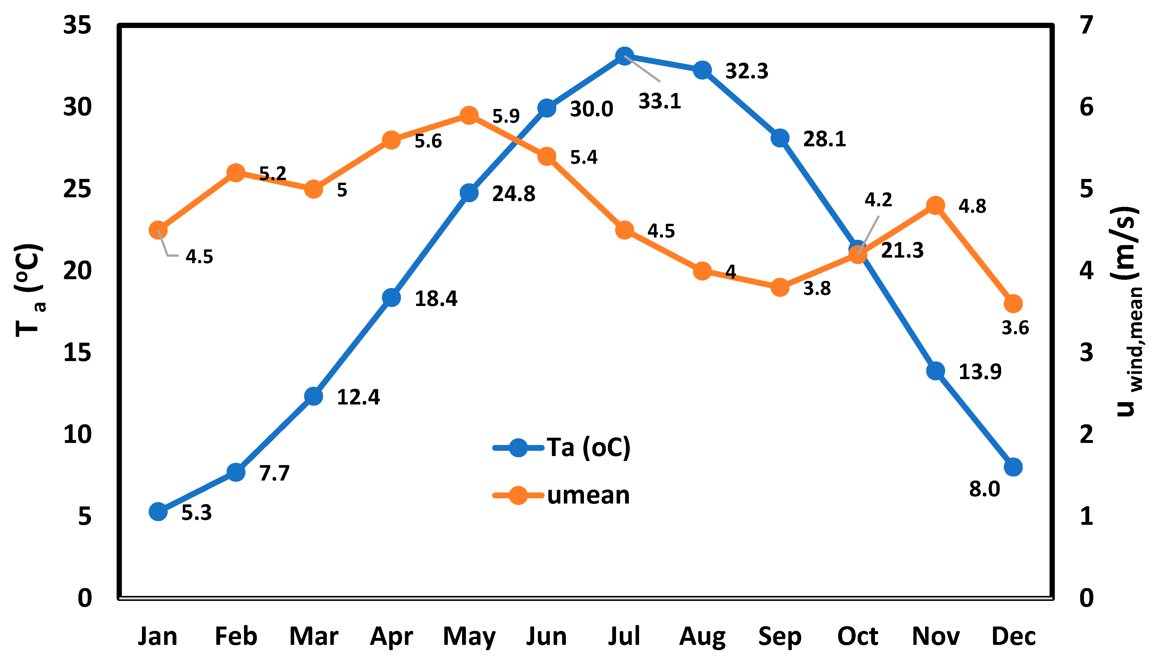
• The temperature of the environment was assumed to be 15 $℃$, and the pressure was 101.3 kPa.
• The pressure loss and heat loss were respectively considered to be 3 and 5%.
• In compressors and turbines, the thermodynamic process was polytropic.
• Potential energy and kinetic energy were negligible.
• According to the market, the efficiency of the combustion chamber was 92%.
• The terminal pressure loss was presumed to be 3% through the pipe
• Heat loss of components was assumed around 3% of the energy released by the hottest steam at these components.
• According to the market, the efficiencies of the RC turbine and pump were considered to be 85%.
• According to the market, the energy efficiencies of the condenser and evaporator were considered to be 85%.
• According to the market, the efficiencies of the gas turbine, compressor, and booster compressor were 88%, 87%, and 87%, respectively.

For each component of both systems, energy and mass conservation laws were applied, which are presented as follows [30]:

$$\frac{\mathrm{dm}}{\mathrm{dt}}={\displaystyle \sum }_{\mathrm{in}}ṁ-{\displaystyle \sum }_{\mathrm{out}}ṁ$$

(1)

$$\stackrel{.}{\mathrm{Q}}-Ẇ={\displaystyle \sum }_{\mathrm{out}}ṁ\left(\mathrm{h}+\frac{{\mathrm{V}}^2}{2}+\mathrm{gZ}\right)-{\displaystyle \sum }_{\mathrm{in}}ṁ\left(\mathrm{h}+\frac{{\mathrm{V}}^2}{2}+\mathrm{gZ}\right)$$

(2)

Here ${ṁ}_{}$ and h represent mass flow rate and specific enthalpy. $\stackrel{.}{\mathrm{Q}}$ and $Ẇ$ are heat and work transfer rate. V, g, and Z are velocity, gravitational acceleration, and height.

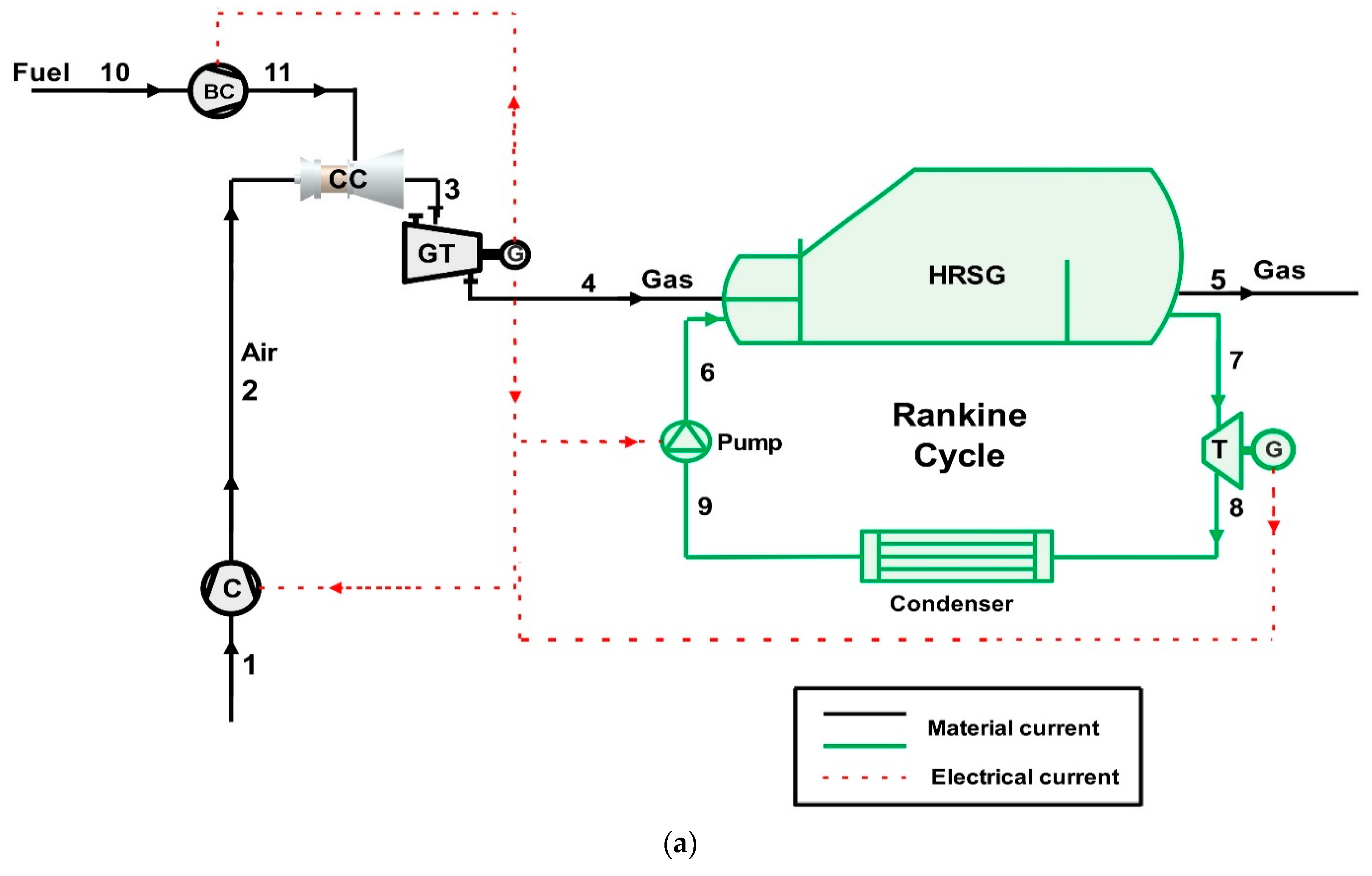
For the combustion chamber of the system (a), GT-HRSG, the following equation can be expressed:

$${ṁ}_2{\mathrm{h}}_2+{ṁ}_{11}\mathrm{LHV}={ṁ}_3{\mathrm{h}}_3+\left(1-{\eta }_{\mathrm{CC}}\right){ṁ}_{11}\mathrm{LHV}$$

(3)

In which, LHV denotes the low heating value of natural gas, for which the molar compositions can be found in

Table 1. The natural gas molar composition [31].

No.	Component	Mixture (mole%)
1	CH4	81
2	C2H6	7.9
3	C3H8	4.2
4	C4H10	4.7
5	CO2	1.2
6	N2	1.0

. Other symbols and subscripts are mentioned earlier.

Using Table 1, the calculations that occur in the combustion chamber can be obtained as follows:

$$\begin{gathered} \frac{1}{r_a}{C}_{x1}{H}_{y1}+(x_{o_2}{O}_2+x_{N_2}{N}_2)\to y_{C{O}_2}C{O}_2+y_{N_2}{N}_2+y_{o_2}{O}_2+y_{H_{2}O}{H}_{2}O \\ {r}_a=\frac{n_{Air}}{n_{Fuel}} \\ {y}_{O_2}=x_{O_2}-\frac{x_1}{r_a}-\frac{y_1}{4r_a} \\ {y}_{N_2}=x_{N_2} \\ {y}_{C{O}_2}=(\frac{x_1}{r_a}+x_{C{O}_2}) \\ {y}_{H_{2}O}=x_{H_{2}O}+\frac{y_1}{2r_a} \end{gathered}$$

(4)

In Equation (4), $r_a$ denotes the air to fuel ratio, and $y_i$ and $x_i$ are a mole and mass fraction of i. The mass and energy balance equations for components of the GT-HRSG combined system are listed in

Table 2. Equations of mass and energy balances for GT-HRSG combined system [31,32].

No.	Component	Mass Balance	Energy Balance
Gas cycle
1	Combustion chamber	${ṁ}_2+{ṁ}_{11}={ṁ}_3$	${ṁ}_2{h}_2+{ṁ}_{11}{h}_{11}={ṁ}_3{h}_3$
2	Gas turbine	${ṁ}_3={ṁ}_4$	${\dot{\mathrm{W}}}_{GT}={\dot{\mathrm{m}}}_3\left(h_3-h_4\right){\eta }_{GT}$
3	Compressor 1	${ṁ}_1={ṁ}_2$	${\dot{\mathrm{W}}}_{comp}=\frac{{\dot{\mathrm{m}}}_1\left(h_2-h_1\right)}{{\eta }_{comp}}$
4	Booster compressor	${ṁ}_{10}={ṁ}_{11}$	${\dot{\mathrm{W}}}_{BC}=\frac{{\dot{\mathrm{m}}}_{10}\left(h_{11}-h_{10}\right)}{{\eta }_{BC}}$
Rankine cycle
5	HRSG	${\dot{\mathrm{m}}}_6={\dot{\mathrm{m}}}_7;{\dot{\mathrm{m}}}_4={\dot{\mathrm{m}}}_5$	${\dot{\mathrm{m}}}_4\left(h_4-h_5\right)={\dot{\mathrm{m}}}_6\left(h_7-h_6\right)$
6	Turbine	${ṁ}_7={ṁ}_8$	${\dot{\mathrm{W}}}_T={\dot{ \mathrm{m}}}_7\left(h_7-h_8\right){\eta }_T$
7	Condenser	${ṁ}_9={ṁ}_8$	${\dot{\mathrm{Q}}}_{cond}={ṁ}_8\left(h_9-h_8\right)$
8	Pump	${\dot{\mathrm{m}}}_9={\dot{\mathrm{m}}}_6$	${\dot{\mathrm{W}}}_P=\frac{{\dot{\mathrm{m}}}_9\left(h_{6s}-h_9\right)}{{\eta }_P}$

.

In Table 2, $\eta$ is efficiency, and subscripts T, GT, comp, BC, cond, and p respectively define the turbine, the gas turbine, the compressor, the booster compressor, the condenser, and the pump. For GC stand-alone, the net electricity production can be obtained as follows:

$${\dot{\mathrm{W}}}_{GC,net}={\dot{\mathrm{W}}}_{GT}-{\dot{\mathrm{W}}}_{comp}-{\dot{\mathrm{W}}}_{BC}$$

(5)

In which, subscript GT is the gas turbine, and ${\dot{\mathrm{W}}}_{comp}$ and ${\dot{\mathrm{W}}}_{BC}$ define the power requirement of the compressor and the booster compressor. For the combined cycle, the net power production is achieved as follows:

$${\dot{\mathrm{W}}}_{CC,net}={\dot{\mathrm{W}}}_{GT}+{\dot{\mathrm{W}}}_T-{\dot{\mathrm{W}}}_{comp}-{\dot{\mathrm{W}}}_{BC}-{\dot{ \mathrm{W}}}_P$$

(6)

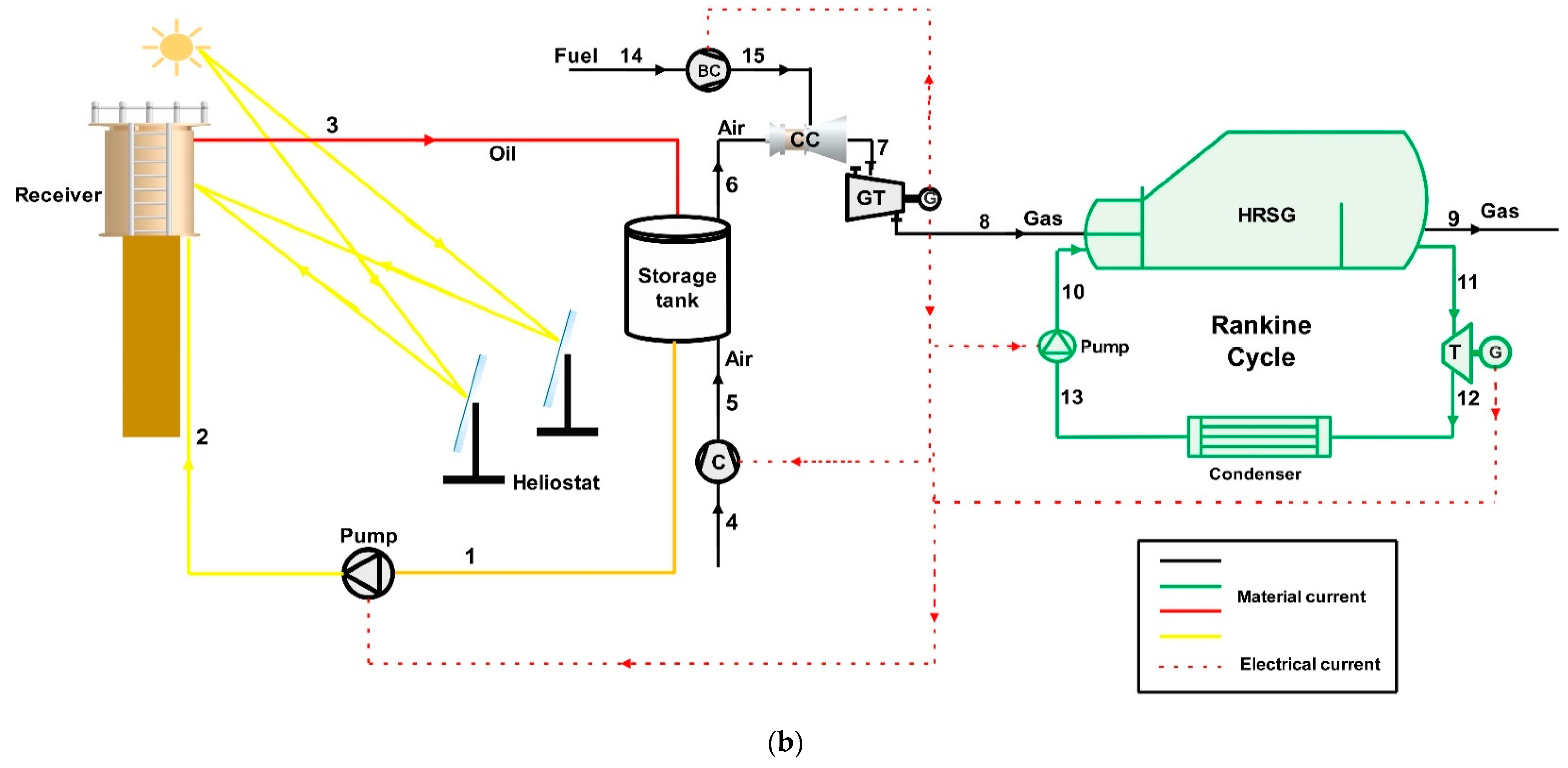
For system (b), GT-HRSG-HSR, the energy, and mass balance equations of the gas and Rankine cycles are similar to Table 2 presented for the GT-HRSG system except for the change in streams’ number. The mass and energy balances for the HSR system are presented in

Table 3. Equations of mass and energy balances for the HSR cycle [33,34,35].

No.	Component	Mass Balance	Energy Balance
HSR Cycle
1	Receiver	${ṁ}_2={ṁ}_3$	${\dot{\mathrm{m}}}_1\left(h_3-h_2\right)={\dot{ \mathrm{Q}}}_S$
2	Pump	${\dot{\mathrm{m}}}_1={\dot{\mathrm{m}}}_2$	${\dot{\mathrm{W}}}_P=\frac{{\dot{\mathrm{m}}}_1\left(h_{2s}-h_1\right)}{{\eta }_P}$
3	Storage Tank	${ṁ}_3+{ṁ}_5={ṁ}_1+{ṁ}_6$	${\dot{\mathrm{m}}}_1\left(h_3-h_1\right)={\dot{\mathrm{m}}}_6\left(h_6-h_5\right)$

.

First and foremost, for solar radiation modeling, solar time can be achieved from the following equation [36]:

$$Solartime=Standardtime+E-4\left(L_{st}-L_{loc}\right)$$

(7)

In which, $L_{st}$ and $L_{loc}$ are respectively local zone time standard meridian, and location longitude. Moreover, the parameter E from equation above is given as [36]:

$$E=229.2\left(0.000075+0.001868Cos\beta -0.04089Sin2\beta -0.014615Cos-0.032077Sin\beta \right)$$

(8)

$$\beta =\frac{\left(n-1\right)360}{365}$$

(9)

Here, n is equal to 1 on the first of January.

Sunset hour angle is another key parameter that can be formulated as follows [36]:

$$\omega =\mathit{arccos}\left(tan\left(\phi \right)tan\left(\delta \right)\right)$$

(10)

Here, $\phi$ and $\delta$ denote latitude and deflection angles, respectively. The deflection angle is calculated using the following equation [37]:

$$\delta =23.45sin\left(\frac{360\left(284+n\right)}{365}\right).$$

(11)

In which, n is equal to 1 on the first of January.

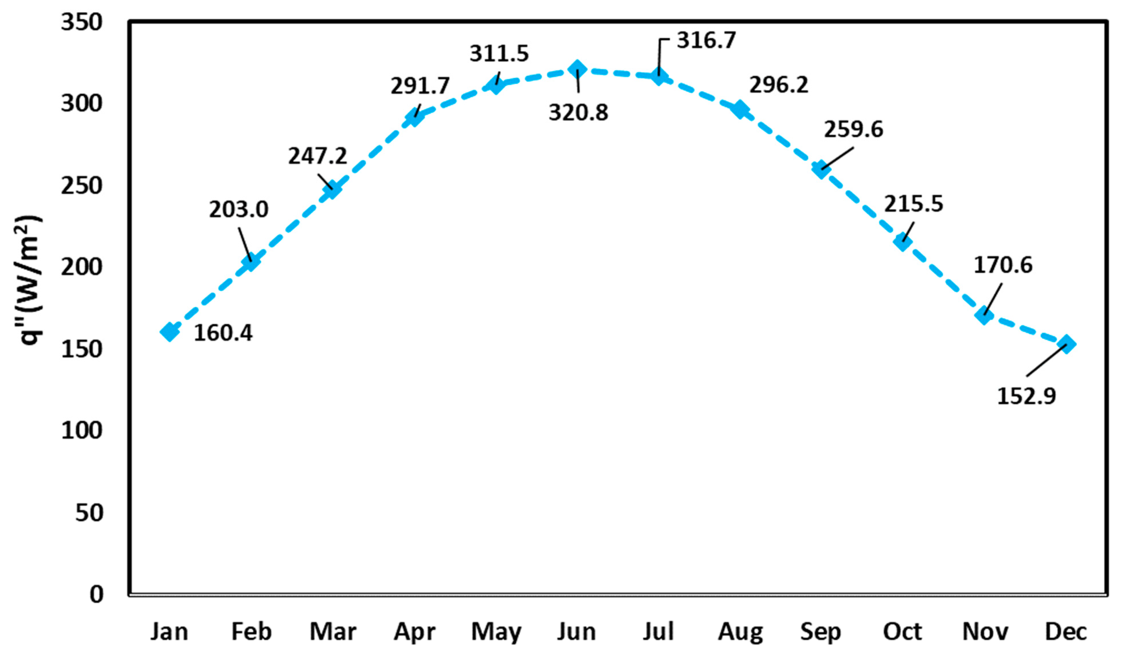
The solar direct beam irradiation can be obtained as follows [37]:

$$G_b=Acos\left({\theta }_z\right)exp\left(\frac{-B}{cos\left({\theta }_z\right)}\right)$$

(12)

Here, A and B are constants that can be found in Reference [37], and ${\theta }_z$ represents a solar zenith angle. Detailed information can be found in Reference [37,38].

For the heliostat field solar receiver, the following equation is formulated for calculation of total heat absorbed by the solar receiver [39]:

$${\dot{\mathrm{Q}}}_{net}={\dot{\mathrm{Q}}}_S-{\dot{\mathrm{Q}}}_{loss}$$

(13)

In which, ${\dot{\mathrm{Q}}}_{net}$ is of total heat rate absorbed by the solar receiver, ${\dot{\mathrm{Q}}}_S$ and ${\dot{\mathrm{Q}}}_{loss}$ are the solar energy input rate, and losses rate. The equation regarding heat loss rate can be expressed as [39]:

$${\dot{\mathrm{Q}}}_{loss }={\dot{\mathrm{Q}}}_{loss,rad}+{\dot{\mathrm{Q}}}_{loss,conv}$$

(14)

Here, ${\dot{\mathrm{Q}}}_{loss,rad}$ and ${\dot{\mathrm{Q}}}_{loss,conv}$ are thermal energy losses associated with radiation and convection.

For the radiation form of thermal power losses, the following equation can be applied [39]:

$${\dot{\mathrm{Q}}}_{loss,rad}=\sigma ·{\epsilon }_{re}·A_{re}\left(T_{re}{}^4-T_{am}{}^4\right)$$

(15)

In Equation (15), $T_{re}$ and $T_{am}$ denotes the temperature of the receiver and the ambient environment. $A_{re}$ and ${\epsilon }_{re}$ denote the area of the receiver and surface emissivity of the receiver. $\sigma$ represent the Stefan Boltzmann constant. The subscript redefines the receiver.

Additionally, the convection form of the thermal power losses is given as [39]:

$${\dot{\mathrm{Q}}}_{loss,conv}=h_{forced}·A_{re}\left(T_{re}-T_{am}\right)$$

(16)

Here, $h_{forced}$ denotes the forced heat transfer coefficient of convection. Further information can be found in Reference [39].

For the solar energy radiation absorbed by an HSR in Equation (13), the following equation can be used [40]:

$${\dot{\mathrm{Q}}}_S={\eta }_{opt}\alpha A_{ap}{G}_b$$

(17)

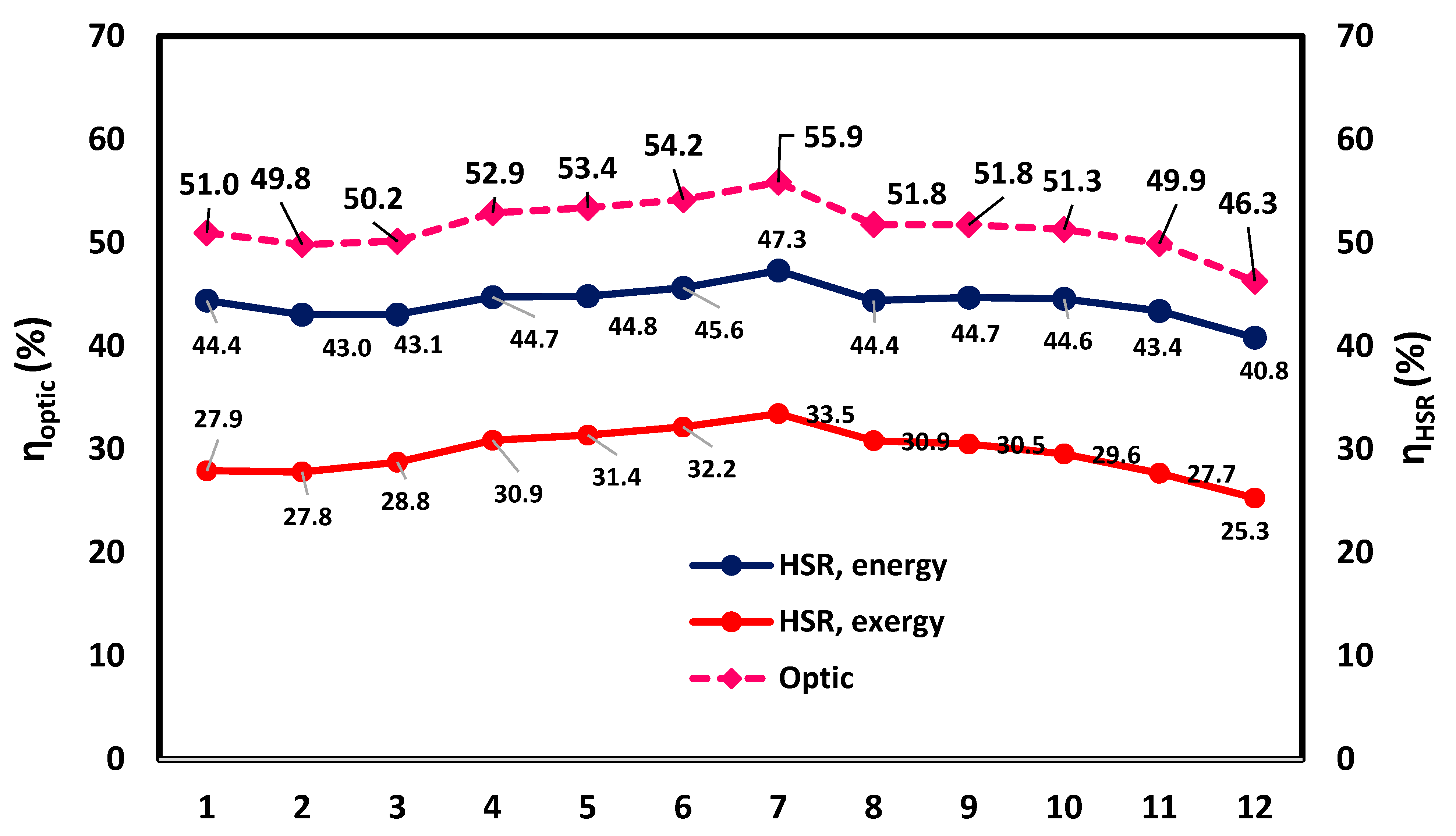
Here, $\alpha$ denotes the solar receiver absorption factor, and ${\eta }_{opt}$ is the optic efficiency of the heliostat. $A_{ap}$ defines the total area of the aperture. Additionally $G_b$ represents the solar direct beam irradiation presented in Equation (12).

The optic efficiency of heliostat (${\eta }_{opt}$) can be formulated as follows [41]:

$${\eta }_{opt}={\eta }_{ref}\times {\eta }_{s\&b}\times {\eta }_{at}\times {\eta }_{spillage}\times {\eta }_{cos}$$

(18)

Here, ${\eta }_{ref}$ denotes the efficiency of the mirror reflectivity rate that is assumed to be 95% in this study [41]. ${\eta }_{s\&b}$ is the efficiency of shadowing and blocking, ${\eta }_{at}$ represents the efficiency of atmospheric attenuation, ${\eta }_{spillage}$ defines the efficiency of spillage, and ${\eta }_{cos}$ is the cosine efficiency.

The shadowing and blocking efficiency, the blocking defines as a heliostat blocks a heliostat in the backside. Additionally, the shadowing occurs as a heliostat casts the shadow on an adjacent heliostat. In this study, the shadowing and blocking efficiency was assumed to be 95% [42].

The atmospheric attenuation efficiency depends on two parameters, weather conditions and distance of heliostat and the receiver. For a distance more than 1000 m following equation can be expressed [41]:

$${\eta }_{at}=exp{\left(-0.0001106d\right)}^{}$$

(19)

Additionally, for a distance lower than 1000 m the atmospheric attenuation efficiency is given as [41]:

$${\eta }_{at}=0.99321-0.0001176d+1.97\times {10}^{-8}{d}^2$$

(20)

In which d is the distance mentioned.

The cosine efficiency can be calculated using the following equation [43]:

$${\eta }_{cos}=\frac{\sqrt{2}}{2}{\left(1+sin({\alpha }_s)·cos\left({\lambda }_s\right)-cos\left({\phi }_{surf}-{\phi }_s\right)·cos\left({\alpha }_s\right)·sin({\lambda }_s)\right)}^{0.5}$$

(21)

In which, ${\alpha }_s$ represents the solar altitude angle [44], ${\lambda }_s$ denotes angle between reflected irradiations and vertical direction [43], ${\phi }_s$ and ${\phi }_{surf}$ are respectively the solar azimuth angle, and the angle of the surface [45]. For further information Reference [46,47] can be used.

Additionally, the spillage efficiency defines the failure of receiving reflected radiation of the heliostat field by the receiver is given as [48]:

$${\eta }_{spillage}={{\displaystyle \int }}_{-r_{ap}}^{r_{ap}}{f}_1\times d_{}$$

(22)

In which, $r_{ap}$ denotes the aperture effective size of the receiver, $f_1$ is a parameter adapted from Reference [48]. Further information about the calculation of $r_{ap}$ can be found in Reference [48]. Therefore, using the above-mentioned equations, the solar energy input in Equation (17) can be achieved.

The heliostat energy efficiency is calculated by the following equation:

$${\eta }_{energy,HSR}=\frac{{\dot{\mathrm{Q}}}_{net}}{A_{ap}{G}_b}$$

(23)

The working fluid employed in the cycle of the heliostat field solar receiver is Therminol-VP1, which its properties are presented in

Table 4. Therminol VP-1 properties [49].

No.	Parameter	Unit	Value
1	Average Molecular Weight	g/mol	166
2	Enthalpy at 15 $℃$	kJ/kg	4.7
3	Viscosity at 15 $℃$	kg/m·s	0.005051
4	Heat Capacity at 15 $℃$	kJ/kg·K	1.529
5	Crystallizing Point	$℃$	12
6	Normal Boiling Point	$℃$	257
	Thermal Conductivity at 15 $℃$	W/m·K	0.1367
8	Density at 15 $℃$	kg/m3	1069
9	Maximum Bulk Temperature	$℃$	400
10	Flash Point COC	$℃$	124
11	Flash Point PMCC	$℃$	110
12	Composition	-	Biphenyl/diphenyl oxide eutectic mixture

[49].

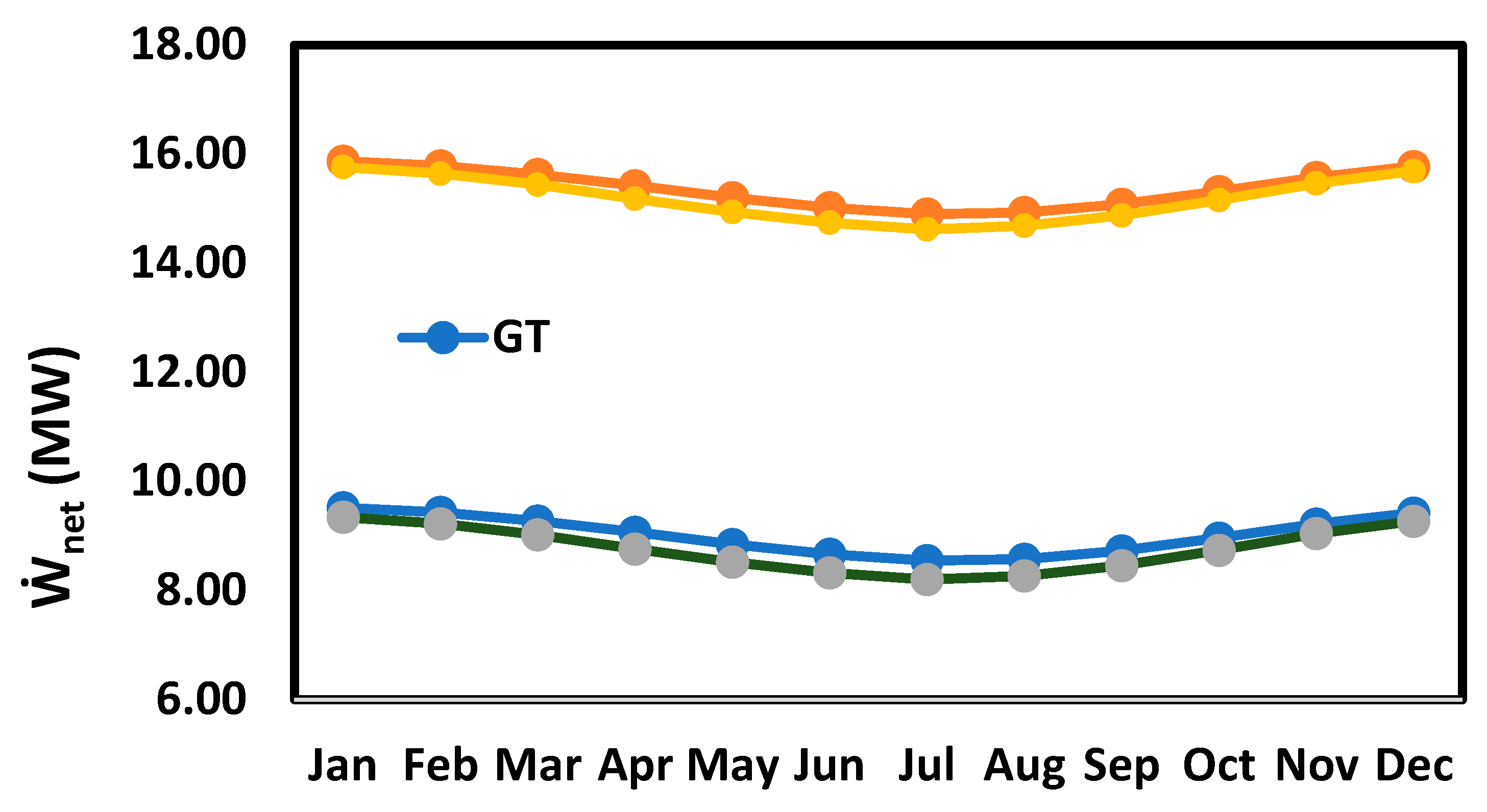
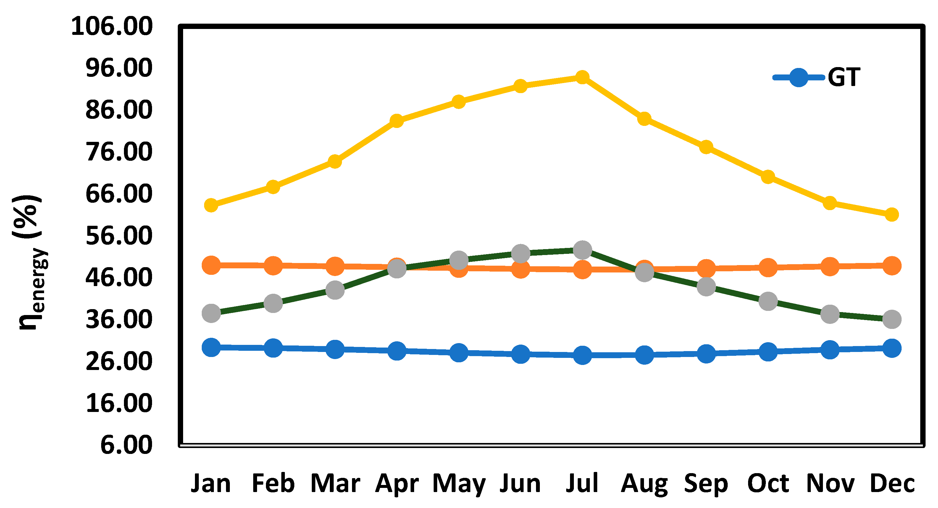
The energy efficiencies of GT and combined cycle were calculated as follows:

$${\eta }_{energy,GT}=\frac{{\dot{\mathrm{W}}}_{net,GT}}{{\dot{\mathrm{m}}}_{10}LHV}$$

(24)

$${\eta }_{energy,CC}=\frac{{\dot{\mathrm{W}}}_{net,CC}}{{\dot{\mathrm{m}}}_{10}LHV}$$

(25)

The above-mentioned equations can be considered in whether to use an HSR cycle or not. The solar radiation was considered in the analysis. The following equation can be proposed for the energy efficiency of the GT-HRSG-HSR system:

$${\eta }_{energy,HSR-GT-HRSG}=\frac{{\dot{\mathrm{W}}}_{net,CC}}{{\dot{\mathrm{m}}}_{f}LHV+{\dot{\mathrm{Q}}}_S}$$

(26)

In this equation, the nominator is the output power of a combined cycle and the dominator is the energy input rate of fuel gas and solar radiation.

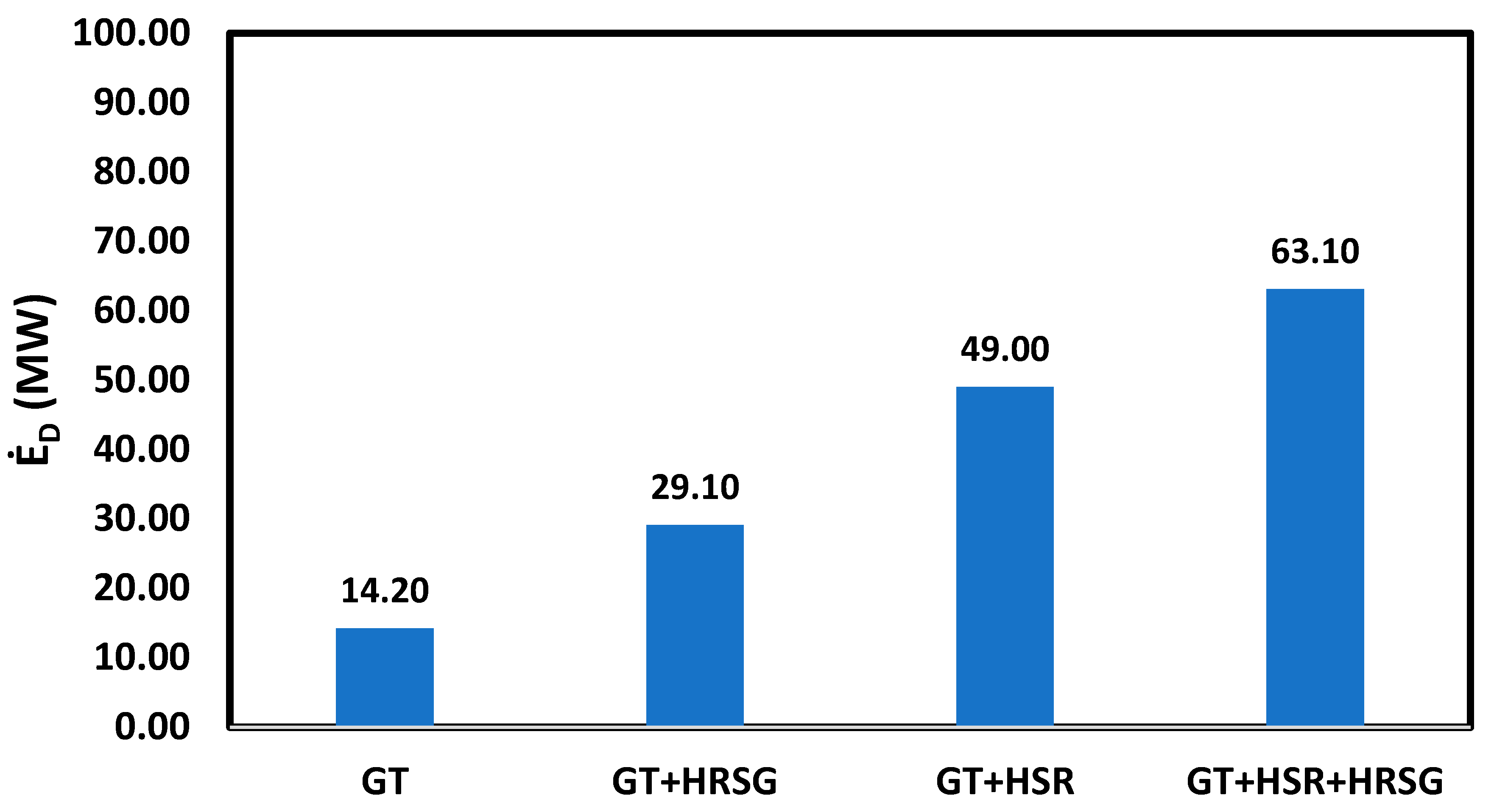
2.3. Exergy Balances

Exergy analysis as a potent tool provides information about inefficiencies in a system that can lead to performance enhancement. Generally, exergy includes four parts; physical, chemical, potential, and kinetic. Specific exergy can be formulated as follows [50]:

$$ex=\left(h-h_0\right)-T_0\left(s-s_0\right)+\frac{V^2}{2}+gz+{{\displaystyle \sum }}^{}{x}_{i}e{x}_{che}+T_0{{\displaystyle \sum }}^{}{x}_i{R}_{i}ln{y}_i$$

(27)

Here, h, T, and s are specific enthalpy, temperature, and specific entropy. $x_i$ and $y_i$ are mass and molar fraction. $e{x}_{che}$ defines the chemical exergy, and $R$ denotes the gas constant. Subscript 0 refers to ambient conditions. Other parameters are described earlier. As mentioned, the potential and kinetic exergies were ignored in this study, and only the physical and chemical exergy was considered. The equations of exergy balance and exergy destruction rate for the GT-HRSG integrated system’s components are listed in

Table 5. Equations of exergy balance and exergy destruction rate for the GT-HRSG integrated system [31,32].

No.	Component	Exergy Efficiency	Exergy Destruction rate
Gas cycle
1	Combustion Chamber	$\frac{{\dot{\mathrm{m}}}_{3}e{x}_3}{{\dot{\mathrm{m}}}_{2}e{x}_2+{ṁ}_{11}e{x}_{11}}$	${\dot{\mathrm{m}}}_{2}e{x}_2+{ṁ}_{11}e{x}_{11}-{\dot{\mathrm{m}}}_{3}e{x}_3$
2	Gas Turbine	$\frac{{\dot{\mathrm{W}}}_{GT}}{{\dot{\mathrm{m}}}_{3}e{x}_3-{\dot{\mathrm{m}}}_{4}e{x}_4}$	${\dot{\mathrm{m}}}_{3}e{x}_3-{\dot{\mathrm{m}}}_{4}e{x}_4-{\dot{\mathrm{W}}}_{GT}$
3	Compressor	$\frac{{\dot{\mathrm{m}}}_2\left(e{x}_2-e{x}_1\right)}{{\dot{\mathrm{W}}}_{comp}}$	${\dot{\mathrm{m}}}_{1}e{x}_1+{\dot{\mathrm{W}}}_{comp}-{\dot{\mathrm{m}}}_{2}e{x}_2$
4	Booster Compressor	$\frac{{\dot{\mathrm{m}}}_{10}(e{x}_{11}-e{x}_{10})}{{\dot{\mathrm{W}}}_{BC}}$	${\dot{\mathrm{m}}}_{10}e{x}_{10}+{\dot{\mathrm{W}}}_{BC}-{\dot{\mathrm{m}}}_{11}e{x}_{11}$
Rankine cycle
5	HRSG	$\frac{{\dot{\mathrm{m}}}_6\left(e{x}_7-e{x}_6\right)}{{\dot{\mathrm{m}}}_4\left(e{x}_4-e{x}_5\right)}$	${\dot{\mathrm{m}}}_4\left(e{x}_4-e{x}_5\right)-{\dot{\mathrm{m}}}_6\left(e{x}_7-e{x}_6\right)$
6	Turbine	$\frac{{\dot{\mathrm{W}}}_T}{{\dot{\mathrm{m}}}_{7}e{x}_7-{\dot{\mathrm{m}}}_{8}e{x}_8}$	${\dot{\mathrm{m}}}_{7}e{x}_7-{\dot{\mathrm{m}}}_{8}e{x}_8-{\dot{\mathrm{W}}}_T$
7	Condenser	$\frac{{\dot{\mathrm{Q}}}_{cond}\left(1-\frac{T_0}{T_{cond}}\right)}{{\dot{\mathrm{m}}}_8\left(e{x}_8-e{x}_9\right)}$	${\dot{\mathrm{m}}}_8\left(e{x}_8-e{x}_9\right)-{\dot{\mathrm{Q}}}_{cond}\left(1-\frac{T_0}{T_{cond}}\right)$
8	Pump	$\frac{{\dot{\mathrm{m}}}_9\left(e{x}_6-e{x}_9\right)}{{\dot{\mathrm{W}}}_p}$	${\dot{\mathrm{m}}}_9\left(e{x}_6-e{x}_9\right)-{\dot{\mathrm{W}}}_p$

.

In

Table 6. Equations of exergy balance and exergy destruction rate for the HSR cycle [33,34,35].

No.	Component	Exergy Efficiency	Exergy Destruction Rate
HSR Cycle
1	Receiver	$\frac{{\dot{\mathrm{Q}}}_{net}\left(1-\frac{T_0}{T_{re}}\right)}{\dot{\mathrm{m}}\left(e{x}_2-e{x}_3\right)+{\dot{Ex}}_{Qs}}$	$\dot{\mathrm{m}}\left(e{x}_2-e{x}_3\right)+{\dot{\mathrm{Q}}}_{loss}\left(1-\frac{T_0}{T_{re}}\right)$
2	Pump	$\frac{{\dot{\mathrm{m}}}_1\left(e{x}_2-e{x}_1\right)}{{\dot{\mathrm{W}}}_p}$	$\dot{\mathrm{m}}\left(e{x}_1-e{x}_2\right)+{\dot{\mathrm{W}}}_P$
3	Storage Tank	$\frac{\dot{\mathrm{m}}\left(e{x}_3-e{x}_1\right)}{\dot{\mathrm{m}}\left(e{x}_6-e{x}_5\right)}$	$\dot{\mathrm{m}}\left(e{x}_3-e{x}_1\right)-\dot{\mathrm{m}}\left(e{x}_6-e{x}_5\right)$

, symbols and subscripts are similar to Table 5, which was earlier presented. Similar to the exergy balance of the GT-HRSG combined cycle, for Rankine and gas cycles of system (b), GT-HRSG-HSR exergy efficiency equations and exergy destruction rates can be formulated. For the HSR cycle, Table 6 can be used for exergy efficiency and exergy destruction rate equations.

In

Table 7. Cost functions of installation and capital investment.

No.	Component	Cost Function ($)	Reference
Gas Cycle
1	Combustion Chamber	$\frac{28.98{\dot{\mathrm{m}}}_2}{0.995-\frac{P_3}{P_2}}(1+exp\left(0.015T_3-1540\right)$	[55]
2	Gas Turbine	$\left(\frac{301.45{\dot{\mathrm{m}}}_3}{0.94-{\eta }_{GT}}\right)ln\left(\frac{P_3}{P_4}\right)(1+exp\left(0.025T_3-1570\right)$	[55]
3	Compressor	$\frac{44.71{\dot{\mathrm{m}}}_1}{0.95-{\eta }_{comp}}\left(\frac{P_2}{P_1}\right)ln\left(\frac{P_2}{P_1}\right)$	[55]
4	Booster Compressor	$\frac{44.71{\dot{\mathrm{m}}}_{10}}{0.95-{\eta }_{BC}}\left(\frac{P_{11}}{P_{10}}\right)ln\left(\frac{P_{11}}{P_{10}}\right)$	[55]
Rankine cycle
5	HRSG	$4745{\left(\frac{{\dot{\mathrm{m}}}_6\left(h_7-h_6\right)}{log\left(T_4-T_5\right)}\right)}^{0.8}+11820{\dot{\mathrm{m}}}_6+685{\dot{\mathrm{m}}}_4$	[55]
6	Turbine	$\left(\frac{301.45{\dot{\mathrm{m}}}_7}{0.94-{\eta }_T}\right)ln\left(\frac{P_7}{P_8}\right)\left(1+\mathit{exp}\left(0.025T_7-1570\right)\right)$	[55]
7	Condenser	$1773{\dot{\mathrm{m}}}_8$	[55]
8	Pump	$3540{\left({\dot{\mathrm{W}}}_P\right)}^{0.71}$	[55]
HSR cycle
9	Land	$0.62\left(1.5A_{land}+1.8\times {10}^5\right)$	[47,48,56,57]
10	Mirror	$126N_{hel}{A}_{hel}$	[47,48,56,57]
11	Wire	${\displaystyle {\displaystyle \sum }_{i=1}^{100}}{N}_{hel,cell,i}\left[0.031r_{cell,i}+24\sqrt{\frac{A_{hel}}{{\rho }_{cell,i}}}\right]$	[48,56]
12	Tower	$0.78232\times {10}^{6}exp\left(0.01130H_{tow}\right)$	[56,58]
13	Piping	$\left[3600\frac{D_{outer}}{1.31}+420\frac{D_{int}}{0.87}\right]H_{tow}+90000\frac{D_{int}}{0.87}$	[23,48,59]
14	Receiver	$23500A_{re}$	[23,48,59]
15	Storage tank	$1.13\left(155.6E_{TES}^{-0.3540}+10.55\right)$	[60,61]

, ${\dot{Ex}}_{Qs}$ defines the exergy rate of solar energy input given as follows [30,51,52]:

$${\dot{Ex}}_{Qs}=G_b{A}_{ap}\left[1-\frac{4}{3}\left(\frac{T_0}{T_{Sun}}\right)+\frac{4}{3}{\left(\frac{T_0}{T_{Sun}}\right)}^4\right]$$

(28)

In which the $T_0$ and $T_{Sun}$ are the temperature of the environment and the sun.

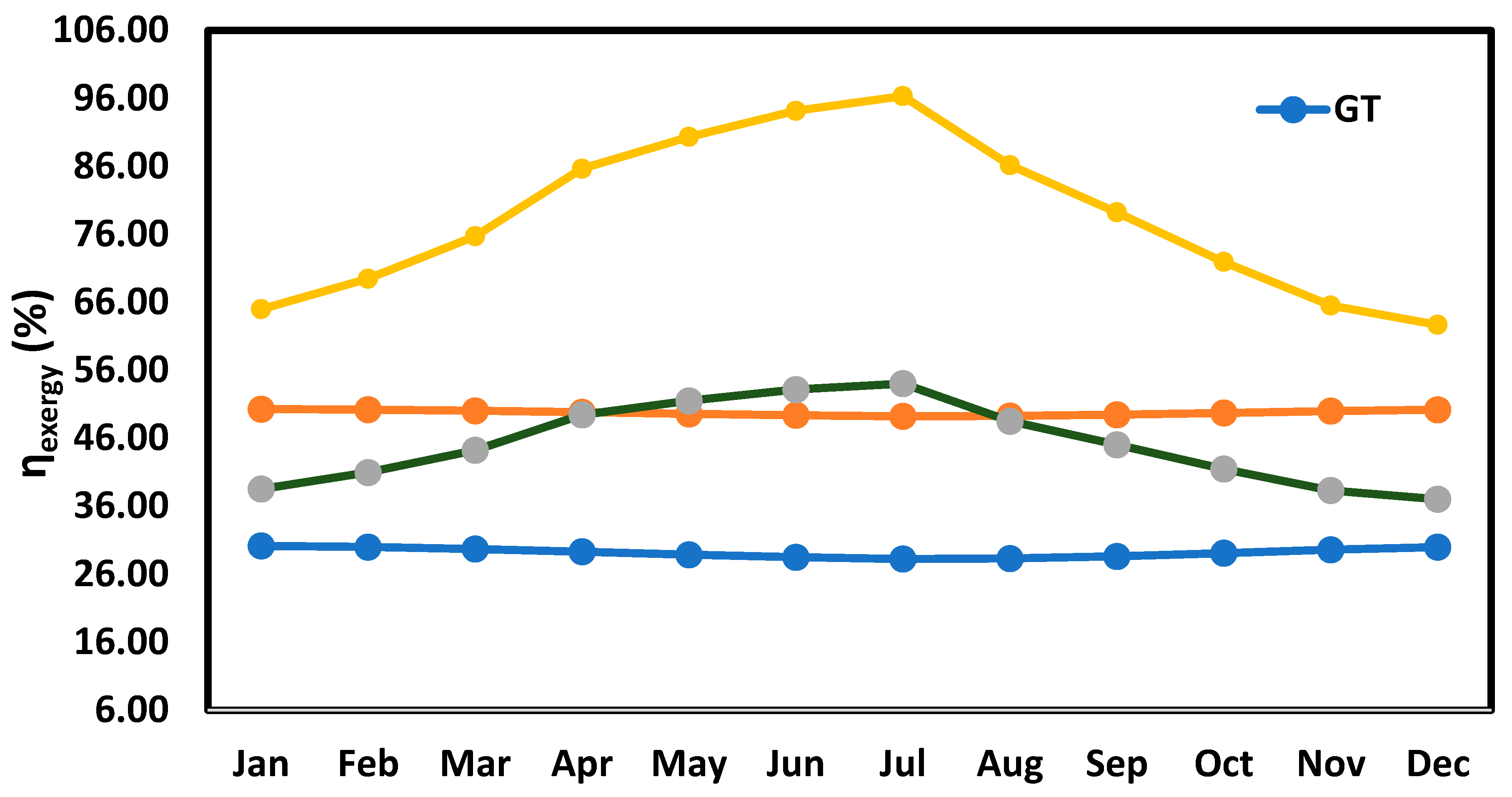
The exergy efficiencies of GT and the combined cycle can be expressed as follows:

$${\eta }_{exergy,GT}=\frac{{\dot{\mathrm{W}}}_{net,GT}}{{ṁ}_{10}e{x}_{10}}$$

(29)

$${\eta }_{exergy,CC}=\frac{{\dot{\mathrm{W}}}_{net,CC}}{{ṁ}_{10}e{x}_{10}}$$

(30)

The above-mentioned equations can be considered in whether to use the HSR cycle or not. The solar radiation was considered in the analysis. The following equation can be proposed for energy efficiency of the GT-HRSG-HSR system:

$${\eta }_{exergy,HSR-GT-HRSG}=\frac{{\dot{\mathrm{W}}}_{net,CC}}{{ṁ}_{10}e{x}_{10}+G_b{A}_{ap}\left[1-\frac{4}{3}\left(\frac{T_{amb}}{T_{Sun}}\right)+\frac{4}{3}{\left(\frac{T_{amb}}{T_{Sun}}\right)}^4\right]}$$

(31)

2.4. Economic Analysis

An economic analysis can be employed to provide the economic performance of a system. To evaluate the economic profitability of two systems, capital investment costs and installation costs were obtained.

The total cost of the one system was calculated by the following equation [53]:

$$Z_{total}=Z_{ins}+Z_{ini}+Z_{OM}+Z_{if}+Z_{cont}+Z_{dec}+Z_{lab}$$

(32)

In which, the subscripts installation, initial, OM, if, cont, dec, and lab denote installation, initial, operation and maintenance, indirect factor, unexpected technological and regulatory issues, decommissioning at the end of the project lifetime, and labor cost. The cost associated with installation cost was about 20% of the initial cost. Operation and maintenance costs were about 4% of the initial cost. The indirect factor, unexpected technological and regulatory issues, and decommissioning at the end of project lifetime were assumed to be 5%, 10%, and 5% of the initial cost of the system [49,54].

The labor costs for the system is given as follows [48]:

$$Z_{lab}=1.5{\displaystyle \sum }_{staff}sa{l}_{stf}{N}_{stf}{N}_{years}$$

(33)

In which, $sa{l}_{stf}$, $N_{stf},$ and $N_{years}$ respectively represent the salary of staff, numbers of staff, and project lifetime that is considered in 20 years. The number 1.5 was considered for extra unpredictable costs.

For an integrated system (a), GT-HRSG, following Table 7 is presented for cost functions of installation and capital investment.

In Table 7, P, ${\dot{\mathrm{W}}}_{}$, and ${\dot{\mathrm{m}}}_{}$ denote pressure, power rate, and mass flow rate. Subscripts GT, comp, BC, T, and P respectively define the gas turbine, the compressor, the booster compressor, the turbine, and the pump. Moreover, $A_{land}$, $A_{hel}$, and $A_{re}$ are respectively the area of the land, heliostat, and receiver. $N_{hel}$ defines the number of heliostats. $N_{hel,cell,i}$ defines the number of the heliostat in cell i, as the field is divided into 100 cells [62].${\rho }_{cell,i}$ denotes the heliostat density in $A_{cell,i}$, which is the area of cell i. $r_{cell,i}$ represents the distance of the cell’s center and the receiver. Further information can be obtained from Reference [47,57,62,63,64]. E_TES is the amount of energy stored in the storage tank [60]. Other subscripts int and outer define the interior and outer to express the diameter (D) of concentric piping. For more information, Reference [23,48,59] can be used.

${\rho }_{cell,i}$ is calculated as follows [48,56]:

$${\rho }_{cell,i}=\frac{N_{hel,cell,i}{A}_{hel}}{A_{cell,i}}$$

(34)

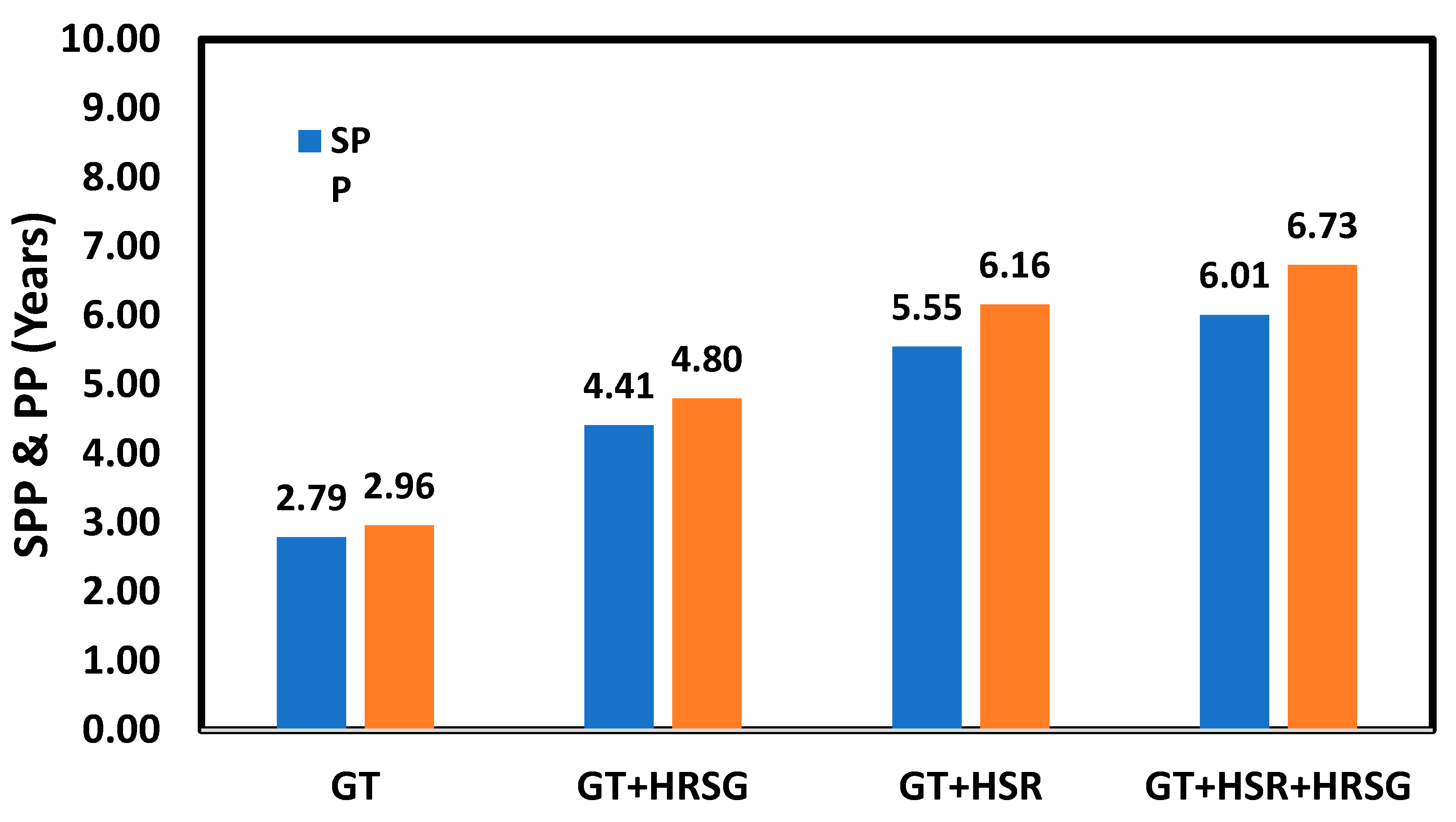
The simple payback period of a system (SPP) is given as [40,65]:

$$SPP=\frac{Z_{total}}{ZF}$$

(35)

In which, Z$F$ defines the cash flow of a system per year.

For the cash flow of both systems per year following equation can be used [40,65]:

$$ZF=Y_{electrical}{k}_{electrical}$$

(36)

Here, the $k_{electrical}$ denotes the specific cost of electricity produced by the systems that is considered equal to 0.22 U$/kWh [65,66]. $Y_{electrical}$ represents the annual electricity production capacity. It should be mentioned that the price of natural gas in this study was 0.07 U$/kWh [67].

For both systems, the payback period (PP) equation can be written as [40,65]:

$$PP=\frac{ln\left(\frac{ZF}{ZF-r·Z_{total}}\right)}{ln\left(1+r\right)}$$

(37)

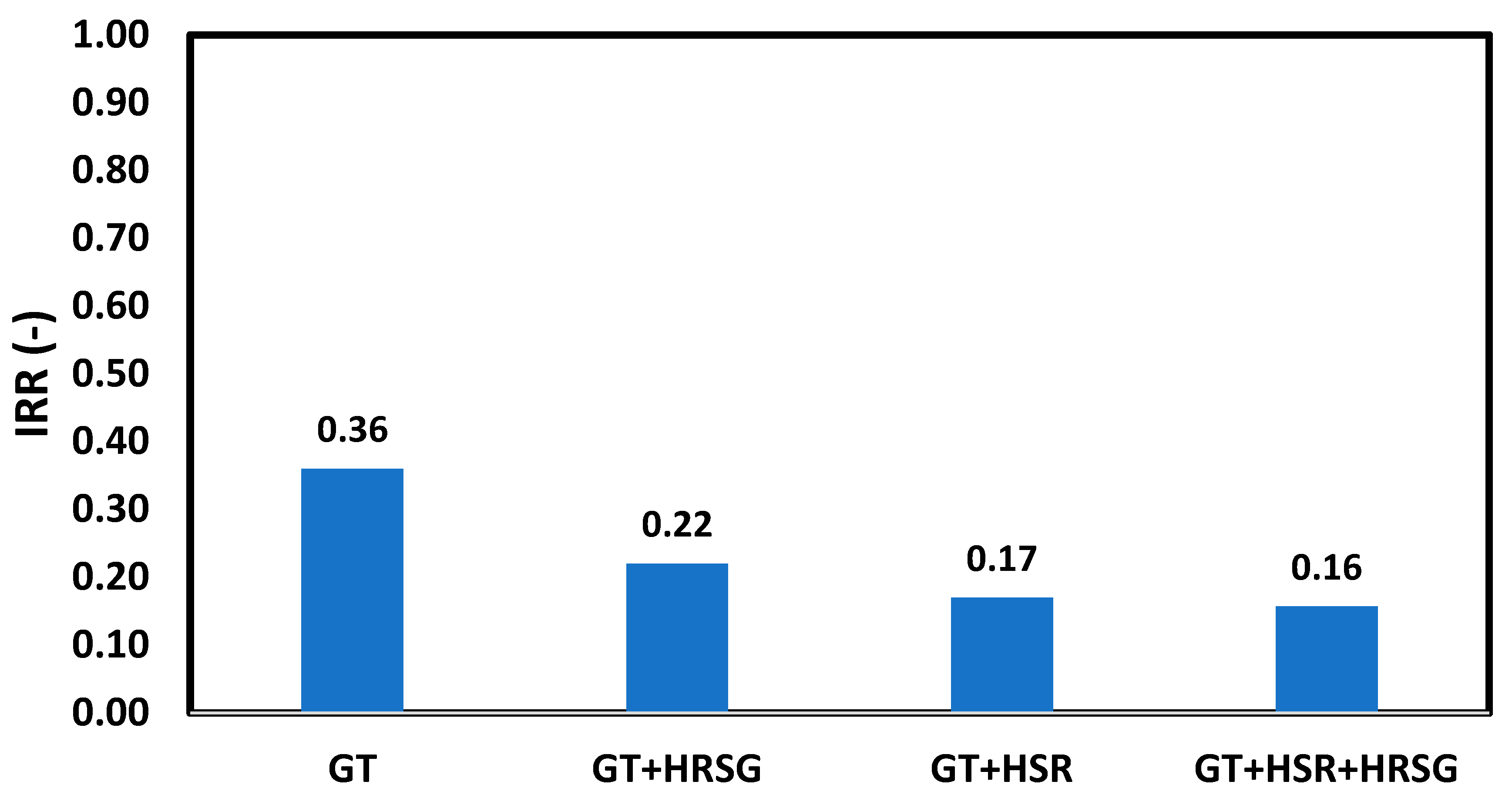
In which, the r is the factor of discount considered as 3% in this study [40,65]. The internal rate of return (IRR) for a system is given as [40,65]:

$$IRR=\frac{ZF}{Z_{total}}\left[1-\frac{1}{{\left(1+IRR\right)}^N}\right]$$

(38)

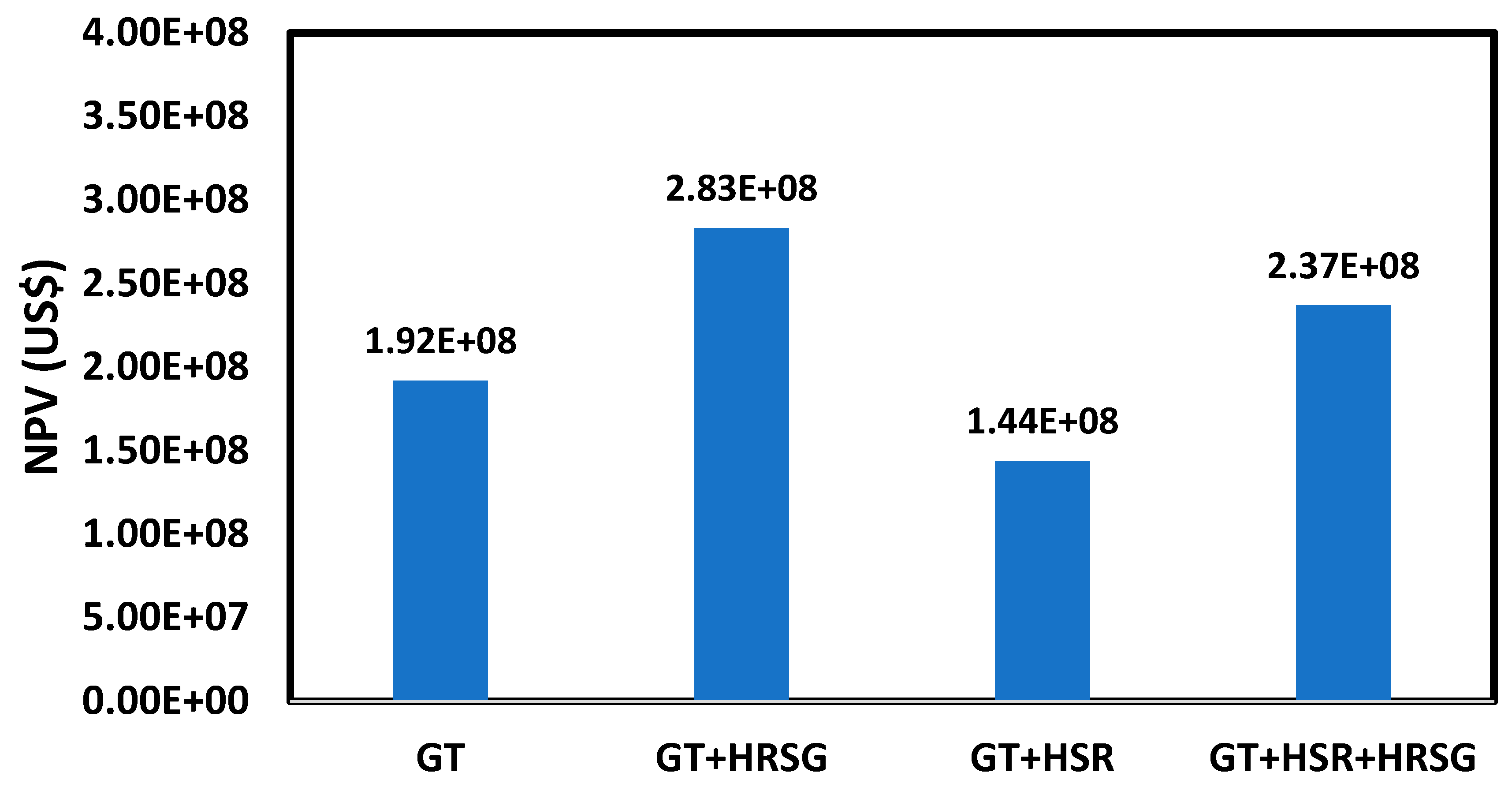
Here, N defines the lifetime of a system that is 20 years in this study. Additionally, the net present value (NPV) of a system can be formulated as follows [40,65]:

$$NPV=ZF\frac{{\left(1+r\right)}^N-1}{r{\left(1+r\right)}^N}-Z_{total}$$

(39)

3. Methodology Section

For the system evaluation, two main computer codes were written in MATLAB software. In one of these codes, the gas cycle and HRSG were modeled without the heliostat solar receiver. In another one, the gas cycle and HRSG were coupled with HSR to investigate the effects of the HSR on the system performance via energy, exergy, and economic aspects. Additionally,, several subroutines were added to the codes. For the first computer code, two subroutines were linked to calculate the natural gas thermodynamic properties. For other working fluids (air and water) the computer code was linked with Refprop software to calculate the thermodynamic properties.

For the second computer code, in addition to the previously mentioned subroutines, three subroutines were added to the computer main code, to calculate the sunrise and sunset times, solar radiation, and Therminol VP-1 thermodynamic properties [50]. Figure 2 shows the block diagram of the main computer program and different subroutines connections.

3.1. Description of the Location of the System

Tehran City is the location considered for both systems. The center of Tehran, Iran, is on latitude $35.689°$ N, and longitude $51.5°$ E. The city has an arid and hot climate, long summers, and cold winters. For the yearly average, the average precipitation is about 230 mm and less than two months of frost. The annual average of sunshine hours and daylight hours of Tehran City are 11 and 13 hours for a day [68,69]. For the 15 July, May, and January, the hourly changes of temperature are illustrated in Figure 3. Generally, the average temperature of July is higher than May followed by January. For July, the maximum temperature is 36.9 $℃$, and the minimum temperature is 23 $℃$. The highest temperature of the fifteenth day of May is 21.6 $℃$, and the lowest temperature is 9.9 $℃$. For January, the maximum temperature is 7.8 $℃$, and the minimum temperature is −5 $℃$. It should be mentioned that the highest temperature of the fifteenth day occurs at 15 o’clock, while the minimum happens at 5 o’clock [65].

As shown in Figure 4, the average temperature and wind speed of each month during a year for Tehran City is presented. This statistical data was based on the measurement for a period of 20 years. January and February had the lowest temperature among all with a temperature of 2.8 $℃$ and 5.1 $℃$. Additionally, the highest temperature was for July with a temperature of 29.35 $℃$, followed by August and June with a temperature of 28.65 $℃$ and 26.2 $℃$ [65]. The lowest wind average velocities were in December and September with an amount of 3.6 m/s and 3.8 m/s. May with 5.9 m/s wind average velocity, April with 5.6 m/s, and June with 5.4 m/s respectively have the highest values [65].

Monthly solar radiation for during a year was exhibited in Figure 5. The variations ranged from 152.9 up to 320.8 W/m². As can be seen, the lowest solar radiation was about 152.9 followed by 160.4 W/m², which occur respectively in December and January. June has the highest solar radiation of about 320.8 W/m², followed by July and May that had 316.7 W/m² and 311.5 W/m² solar radiation [65].

3.2. System Specifications

For the GT-HRSG-HSR system, specifications are presented in

Table 8. The heliostat field solar receiver input parameters.

No.	Parameter	Unit	Value/Definition
1	Total Number of Heliostats	-	1848
2	Working Fluid	-	Therminol VP-I
3	Mass Flow Rate of Working Fluid	kg/s	450
4	Field Layout	-	Radial-staggered/spired
5	Longitude	Degree	51.5 E
6	Latitude Location	Degree	35.689 N
7	Number of Heliostats in the Field	-	1460
8	Number of Heliostats in the First Rows	-	20
9	Field Number of Zones	-	3
10	Distance Between the Receiver Aperture and the Absorbing Aperture	m	9.3
11	Additional Separation Distance between Adjacent Heliostat	m	0
12	Heliostat Vertical Distance from the Ground	m	5
13	Heliostat Width	m	10.5
14	Heliostat Height	m	13.3
15	The Angle of Mirrors	Degree	13
16	Receiver Height	m	12
17	Receiver Radius	m	4.1
18	Tower Optical Height	m	127
19	Inlet Pump Pressure	kPa	101.3

and

Table 9. The systems’ specification [72].

No.	Parameter		Unit	Value
	GT-HRSG	Heliostat-GT-HRSG
1	${\dot{\mathrm{m}}}_1$	${\dot{\mathrm{m}}}_4$	kg/s	27.56
2	$P_{10}$	$P_{14}$	kPa	101.3
3	$T_5$	$T_9$	K	283.5
4	$P_6$	$P_{10}$	kPa	405.2
5	$P_8$	$P_{12}$	kPa	101.3
6	$r_{comp}$		-	11.5
7	${\eta }_{comp}$		-	0.85
8	${\eta }_{BC}$		-	0.76
9	$r_{GT}$		-	12.8
10	${\eta }_{GT}$		-	0.8

[33,34,35,57,62,70,71]. The input parameters of HSR were extracted from references [33,34,35,57,62,70,71] with some minor changes. Additionally, for the GT-HRSG system, Table 9 tabulates the specifications.

In Table 9, $r_{comp}$ and $r_{GT}$ define the pressure ratio of the compressor and the gas turbine.

4. Results and Discussion

In this section, the performance of both systems from energy, exergy, and economic perspectives were reported during a year. Moreover, the energy, exergy, and economic enhancement achieved by adding each cycle to the system is presented for each month of a year.

4.1. Model Validation

Since this cycle was not investigated yet. So, each system was validated individually. For HSR, Reference [47] was considered. Then based on the specific design parameters presented in that reference, the annual thermal energy obtained by HSR was calculated and compared with this value presented in Reference [47]. The annual thermal energy via HSR was calculated around 99.27 GWh that this value was equal to 102.3 GWh. The error was around 3%. For the gas and combined cycles approval, Reference [67] was thought of. There, a basic gas cycle with an HRSG was thought of, and the pinch temperature was 30 K. The most boiler and the base condenser pressures individually were 16 and 0.03 bar. The most extreme superheated steam temperature was 923 K, as in the current framework. The compressor, gas turbine, and steam turbine isentropic efficiencies were 86%, 86%, and 85% separately. The ambient pressure and temperature were 101 kPa and 288 K. The energy efficiency for a combustion temperature of 1375 K was 25%. This parameter was determined by the current model as 23.4%. The error was 6.4%, which is satisfactory.

4.2. HSR (Heliostat Solar Receiver) Results

Figure 6 is dedicated to reporting the monthly average optic efficiency and energy and exergy efficiencies of the heliostat solar receiver in each month of a year. This parameter mainly depends on the field layout and spillage efficiency in comparison to changes associated with different months. This fact can justify the slight changes in this parameter during a year. As can be seen, the changes were between 46.3% and 55.9%. The highest values of average heliostat optic efficiency belong to May, June, and July, which were respectively 53.4%, 54.2%, and 55.9%. Therefore, July had the highest amount. While December had the minimum average heliostat optic efficiency about 46.3% followed by February and November for which the values were about 49.8% and 49.9%.

For energy efficiency, slight changes were observed during a year from 40.8% in December, up to 47.3% in July. According to Equation (23), these slight changes were because both numerator and denominator of energy efficiency were increased by the rising of solar radiation. The exergy efficiency of the heliostat solar receiver was generally lower than the energy efficiency of the system. Based on the equations presented in Table 7, this is because of the $\left(1-\frac{T_0}{T_{re}}\right)$ coefficient that leads to a reduction in the numerator, and also the $\left[1-\frac{4}{3}\left(\frac{T_0}{T_{Sun}}\right)+\frac{4}{3}{\left(\frac{T_0}{T_{Sun}}\right)}^4\right]$ coefficient that leads to an increase of the denominator. The variations of exergy efficiency range from 25.3% in December up to 33.5% in July, which the reason for these small changes during a year is similar to the reason discussed for energy efficiency variations.

Monthly average heat absorbed by the solar receiver, total solar energy input, defined as a tot in the figure, and thermal power losses are shown in Figure 7. As presented in Equation (14), thermal power losses occur by radiation and convection. Based on Equation (13), the average heat absorbed by the solar receiver can be obtained by subtracting the thermal power losses from the total solar energy input presented by Equation (17). Generally, the thermal power losses are enormously lower than the total solar energy input, which is because of a significant amount of solar radiation reflected by large areas of heliostats in comparison to comparatively low thermal power losses from small areas of the solar receiver. As can be seen in Figure 7, the thermal power losses are relatively high in May, June, and July since this parameter is considerably increased by the increase of the wind velocity and air temperature. On the other hand, because of high average solar radiation in May, June, and July, total solar energy input and, as a result, the average heat absorbed by the solar receiver are both high. The maximum average heat absorbed by the solar receiver was about 23.98 MW in July, and the minimum was 10.29 MW occurs in December.

4.3. GC (Gas Cycle) and CC (Combined Cycle) Results

Figure 8 demonstrates the monthly average of net electricity generation in four types, which are GT, GT + HRSG, GT + HSR, and GT + HRSG + HSR. For the GT type, the average of net electricity generation changed from 8.54 MW in July up to 9.51 MW in January. As can be seen, the electricity generation of GT diminished in warm months of a year. As known, in gas cycles, the volume flow rate of a cycle was constant while the gas density was reduced in warm months of a year, which ended up with lower electricity generation. For the GT + HSR type, the monthly average of net electricity generation was lower than the GT type. Since the HSR was employed to preheat the inlet air of the combustion chamber, the mass flow rate of the inlet fuel of the combustion chamber decreased, followed by a decrement of the inlet mass flow rate of the gas turbine, which led to less electricity generation. Clearly, for the GT + HRSG type, because of the heat recovery used for the Rankine cycle significantly higher electricity generation can be achieved. Hence, for the GT + HRSG type, the variations of net electricity generation ranged from 14.9 MW in July up to 15.87 MW in January. Furthermore, when adding the HSR cycle to the GT + HRSG type a slight reduction could be seen, which is justified similarly to adding HSR to the GT type mentioned above.

The monthly average of energy efficiencies of the four mentioned types was exhibited in Figure 9. By comparing the GT cycle and the GT + HSR system, although the monthly average net electricity production of GT + HSR type was lower than the GT type according to Figure 8, the monthly average energy efficiency was higher for the GT + HSR type. This phenomenon is because that by employing the HSR cycle less of a fuel mass flow rate is required in the gas cycle leading to a reduction in the denominator that has a dominance effect in comparison to a decrease of numerator, which is the net electricity generation. Definitely, for the combined cycle or GT + HRSG type, the energy efficiency is higher than GT type due to higher net electricity generation. In warm months of a year, a slight decrease in both GT and GT + HRSG types was observed, which is because of a reduction in the gas density in these months that diminishes the net electricity generation. In the GT + HSR type, for May, June, and July, the energy efficiency was higher than the GT + HRSG type because of an increase of the average absorbed heat rate by the solar receiver in these months. Additionally, the GT + HSRG + HSR or the whole system had a significant energy efficiency between 61% and 93%, particularly in warmer months such as May, June, and July that the energy efficiency maintained being more than 87%.

Figure 10 reports the monthly average of exergy efficiency of four types of GT, GT + HRSG, or the combined cycle, GT + HSR, and GT + HRSG + HSR, or the whole system. The results of monthly average exergy efficiencies were similar to the monthly average energy efficiency presented in Figure 9 with slight changes. Exergy efficiencies of all four types were slightly lower than their energy efficiencies, which were because of the higher value of fuel-specific exergy in comparison to LHV of the fuel in the denominator of the energy and exergy efficiencies’ equation.

In Figure 11, a new concept for energy and exergy efficiencies of the GT + HRSG + HSR was proposed that includes solar radiation. For the energy efficiency of system (b), the solar energy radiation input in Equation (17) was added to the denominator of the equation. Additionally, for the exergy efficiency of this system, the exergy rate of solar energy input presented in Equation (28) was added to the denominator of the exergy efficiency equation. As a result, both monthly average energy and exergy efficiencies were low in comparison to Figure 10 and Figure 11 particularly in the warm month in which the solar radiation was relatively high.

The annual average energy and exergy efficiencies of four types of GT, GT + HRSG, GT + HSR, and GT + HRSG + HSR are shown in Figure 12. The annual average energy efficiency for standalone GT was 28.4%, which could be significantly increased by up to 48.5% by adding HRSG to the GT cycle, which is system (a). Although adding the HSR cycle to the GT could increase the cycle up to 44%, this increment was 9% lower than the energy enhancement achieved by adding the HRSG unit to the GT. This outcome suggests that between adding HRSG and HSR, the annual average energy efficiency of using HRSG was higher. Additionally, for system (b) or GT + HRSG + HSR, the annual average energy efficiency was significantly high about 76.5% revealing the high energy performance of this system. The annual average exergy efficiency for GT type was 29.2% increased up to 49.8 for the GT + HRSG or system (a). For the GT + HSR, the annual average exergy efficiency was slightly lower about 45.2%. Additionally, finally, for system (b) or the GT + HRSG + HSR, the parameter reached 78.5%.

The NPV economic factor for all four types was demonstrated in Figure 13. The NPV for the GT standalone was 1.92 $\times {10}^8$ US$, which experienced a significant increase of up to 2.83 $\times {10}^8$ US$ by adding the HRSG unit presented as system (a). On the other hand, for the GT + HSR type, the NPV factor reduced down to 1.44 $\times {10}^8$ US$, which was 25% lower than NPV of GT type. As higher values of the NPV factor are favorable, this result suggests that adding HSR in comparison to the HRSG unit is not economically advantageous. Additionally, for system (b). GT + HRSG + HSR, the NPV factor was 2.37 US$. Therefore, regarding the economic performance of these types of configurations, the most and the least beneficial system were respectively GT + HSRG and the GT + HSR types.

Figure 14 reports the SPP and PP economic factors for the mentioned four types. The SPP factor of the GT system was 2.79 years, which adding HRSG unit increased this factor to about 58% up to 4.41 years. Additionally, for the GT + HSR type, the SPP factor rose to 5.55 years, which was a 98% increase in comparison to the GT standalone type. Regarding the SPP of the GT + HRSG type, the increase observed in GT + HSR was also 26% higher, which was due to the high capital investment of the HSR cycle and because adding the HSR cycle would decrease the electricity generation presented in Figure 9. Additionally, for system (b) or the GT + HRSG + HSR type, the SPP was increasing up to 6.01 years, which was 36% higher than system (a) or the GT + HRSG type. The PP factor for GT was 2.96 years and increased up to 4.8 years for system (a) or the GT + HRSG type. For the GT + HSR cycle, the PP factor was 6.16 years, and for system (b) or GT + HRSG + HSR, this parameter was found to be 6.73 years. Comparing system (a) and system (b), PP for system (b) was 40% higher than system (a) revealing the fact that system (a) was a superior choice from this economic factor point of view.

Similar to the outcomes of previous figures about the economic performance of the proposed systems, the IRR factor shown in Figure 15 for all four types was justified. The highest IRR belongs to the GT type and the GT + HSR + HRSG type had the lowest value of IRR, and as known the higher values of this economic factor were more desirable. The IRR factor for the GT system was about 0.36, which was decreased by about 39% for system (a) or GT + HRSG. Additionally, for the GT + HSR type, the IRR was about 0.17, which substantiated that adding HSR decreased the IRR factor of the GT standalone system by about 53%.

The annual average exergy destruction rate of four types of GT, GT + HRSG, GT + HSR, and GT + HRSG + HSR are shown in Figure 16. By adding each cycle to the gas cycle, the exergy destruction rate was increased. Since, each cycle had a component and each component had a value of the exergy destruction rate during operation time.

Figure 17 shows the levelized cost of electricity (LCOE) of four types of GT, GT + HRSG, GT + HSR, and GT + HRSG + HSR. The LCOE was increased by adding each individual cycle.

5. Conclusions

In this paper, hybrid integration of a heliostat solar receiver (HSR) and gas turbine cycle, combined cycle (gas-steam cycles), and a heat recovery steam generator (HRSG) were examined for power generation in Tehran (Iran). The application of the heliostat solar receiver was to utilize solar energy to heat the pressurized exhaust air before entering the combustion chamber to produce more steam in the gas cycle (GC) and combined cycle (CC). This action led to less consumption of fossil fuels and less of an environmental effect of these cycles. Additionally, the usage of adding a heat recovery steam generator (HRSG) is to exploit excess heat in the exhaust gas of these cycles for more electricity generation and reducing heat loss. Thermodynamic performance assessment of this study revealed since the energy efficiency for standalone GT was 28.4%, it could be significantly increased by up 76.5% for the combination of GT + HRSG + HSR. Moreover, the exergy analysis of this configuration states since the average exergy efficiency for the GT type was 29.2%, it could be improved up to 49.8 and 78.5% for the GT + HRSG and combination of GT + HRSG + HSR. The economic analysis of this hybrid system shows that the NPV and PP for the GT standalone were 1.92 $\times {10}^8$ US$ and 2.96 years, respectively. These two parameters can be changed to 2.83 $\times {10}^8$ US$, and 4.8 years for GT + HRSG, 1.44 $\times {10}^8$ US$, and 6.16 years for GT + HSR, and 2.37 $\times {10}^8$ US$ and 6.73 years for GT+HRSG + HSR. Furthermore, the IRR factor for the GT cycle was about 0.36, and 0.22 for the GT + HRSG and 0.17 for the GT + HSR and 0.16 for GT + HSR + HRSG.

The thermoeconomic assessment of the combination of heliostat solar receiver (HSR) and Brayton cycle with air and supercritical $C{o}_2$ as a working fluid instead of gas cycle alongside with HRSG and the ORC Rankine cycle can be examined as further work. Additionally, replacement of the absorption chiller with ORC or the application, Kalina cycle, and Goswami cycle instead of the heat recovery steam generator (HRSG) in this combination can be evaluated for future works too.