Article

Impact of the ‘13th Five-Year Plan’ Policy on Air Quality in Pearl River Delta, China: A Case Study of Haizhu District in Guangzhou City Using WRF-Chem

1
School of Intelligent Systems Engineering, Sun Yat-sen University, Guangzhou 510275, China
2
Guangdong Provincial Key Laboratory of Intelligent Transport System, Guangzhou 510275, China
3
Guangdong Provincial Engineering Research Center for Traffic Environmental Monitoring and Control, Guangzhou 510275, China
4
Guangzhou Haizhu District Environmental Monitoring Station, Guangzhou 510220, China
*
Author to whom correspondence should be addressed.
Appl. Sci. 2020, 10(15), 5276; https://doi.org/10.3390/app10155276
Submission received: 6 July 2020 / Revised: 25 July 2020 / Accepted: 27 July 2020 / Published: 30 July 2020
(This article belongs to the Special Issue Advances in Air Quality Monitoring and Assessment)

Abstract

:
Due to increasingly stringent control policy, air quality has generally improved in major cities in China during the past decade. However, the standards of national regulation and the World Health Organization are yet to be fulfilled in certain areas (in some urban districts among the cities) and/or certain periods (during pollution episode event). A further control policy, hence, has been issued in the 13th Five-Year Plan (2016–2020, hereafter 13th FYP). It will be of interest to evaluate the air quality before the 13th FYP (2015) and to estimate the potential air quality by the end of the 13th FYP (2020) with a focus on the area of an urban district and the periods of severe pollution episodes. Based on observation data of major air pollutants, including SO2 (sulphur dioxide), NO2 (nitrogen dioxide), CO (carbon monoxide), PM10 (particulate matter with aerodynamic diameter equal to or less than 10 μm), PM2.5 (particulate matter with aerodynamic diameter equal to or less than 2.5 µm) and O3 (Ozone), the air quality of Haizhu district [an urban district in the Pearl River Delta (PRD), China] in 2015 suggested that typical heavy pollution occurred in winter and the hot season, with NO2 or PM2.5 as the key pollutants in winter and O3 as the key pollutant in the hot season. We also adopted a state-of-the-art chemical transport model, the Weather Research and Forecasting model coupled with Chemistry (WRF-Chem), to predict the air quality in Haizhu District 2020 under different scenarios. The simulation results suggested that among the emission control scenarios, comprehensive measures taken in the whole of Guangzhou city would improve air quality more significantly than measures taken just in Haizhu, under all conditions. In the urban district, vehicle emission control would account more than half of the influence of all source emission control on air quality. Based on our simulation, by the end of the 13th FYP, it is noticeable that O3 pollution would increase, which indicates that the control ratio of volatile organic compounds (VOCs) and nitrogen oxides (NOx) may be unsuitable and therefore should be adjusted. Our study highlights the significance of evaluating the efficacy of current policy in reducing the air pollutants and recommends possible directions for further air pollution control for urban areas during the 13th FYP.

1. Introduction

The quality of ambient air is vital to human health. Air quality management is important for many authorities around the world [1]. The Chinese government has put great effort into mitigating the elevated level of air pollutants in the past decade, especially since the Air Pollution Control Action Plan (APCAP) was issued by the State Council in 2013 [2]. The annual levels of PM2.5, PM10, SO2, and NO2 decreased by 12%, 11%, 20%, and 5%, respectively, in major cities during 2013–2015 [3,4].
However, the effect was highly heterogeneous both spatially and temporally since the national standards of air quality were violated in some districts/towns in cities and during severe pollution episode events. Observation stations in the urban area of Beijing [5], Shanghai [6], and Guangzhou [7,8] recorded heavy pollution episodes in winter (PM10, PM2.5, and NO2 as key pollutants) and/or hot seasons (summer and autumn, O3 as key pollutant) [9,10].
To further tackle the air pollution issue, authorities of national and local level have formulated a series of regulations for the 13th Five-Year Plan (13th FYP) [11,12]. Targets have been set such that, by the end of 13th FYP, the emission of SO2 and NO2 should decrease 15% compared to that in 2015, and the ratio of heavy pollution days in 2020 should reduce 25% compared to that in 2015 [11]. The three national typical air pollution city clusters (Beijing-Tianjin-Hebei, the Yangtze River Delta and the Pearl River Delta (PRD)) have their own targets. For example, for the cities of the PRD region, concentrations of air pollutants (PM2.5, PM10, SO2, NO2, CO, and O3) should meet national secondary air quality standards and the number of heavy pollution day should be zero [11]. Although the emission of the air pollutant from large industrial point sources has been decreasing in the past decade, the emission from traffic has been significantly increasing, which leads to critical challenges in air pollution control. It will be of significance to assess the air quality level in the year before the 13th FYP (2015) and to predict the impact of 13th FYP on air quality by 2020.
Some modelling studies have been conducted to evaluate the potential influence of the 13th FYP policy or the impact of policies on air quality during some major public events. Wang et al. (2016) [13] evaluated the impact of emission control measures on the air quality in the PRD region with WRF-CMAQ (The Weather Research and Forecasting Model-Community Multiscale Air Quality Model) model simulation on emission scenarios (a base case in 2010, two cases in 2020). Liu et al. (2017) [14] assessed the cobenefits (air quality and climate change) of vehicle emission control measures for 2015–2020 in the PRD region. Maji et al. (2018) [15] reported the PM2.5-related mortality under air pollution control policies for China 2020. Yang et al. (2016) [16] analysed the effect of the coal control strategy in China on carbon mitigation and pollutants control for 2020 and 2030. Wang et al. (2015) [17] assessed the air quality situation under the pollution control policy of thermal power plants in China for 2020 with MM5-CMAQ (Fifth-Generation Mesoscale Regional Weather Model-Community Multiscale Air Quality Model). Qui et al. (2017) [18] studied the effect of emission control strategies on air quality of Baotou, China. Cai et al. (2017) [19] researched the impact of the ‘Air Pollution Prevention and Control Action Plan’ on PM2.5 in the Jing-Jin-Ji region from 2012–2020 with WRF-CMAQ. Li et al. (2017) [20] estimated the effect of policies in the ‘13th Five-Year Plan’ period on air pollutants emission of China’s electric power sector. Wei et al. (2017) [21] analysed the impact of policies in Shanxi province, China. Guo et al. (2016) [22] researched the impact of emission control measures on air quality during APEC (Asia–Pacific Economic Cooperation summit) China 2014 with the Weather Research and Forecasting coupled with Chemistry (WRF-Chem). Xu et al. (2013) [23] evaluated the effect of air pollution control policies on air quality during the 16th Asian Games with CMAQ (Community Multiscale Air Quality Model). Shen et al. (2016) [24] analysed the influence of emission control policies on air quality during China’s V-Day parade in 2015. Air quality numerical models (WRF-CMAQ, MM5-CMAQ, WRF-Chem, etc.) and scenario analyses were used widely to evaluate the effectiveness of policies on air quality. These studies only focused on the impact of policies on annual air quality in 2020 or on air quality during some major public events and did not investigate air quality on heavy pollution events.
For heavy pollution, previous works focused on the characteristics and formation of pollution episodes. Tan et al. (2009) [25] investigated the chemical characteristics of haze in Guangzhou (2002–2003, summer and winter) with PM10 samples and gas chromatography-mass spectrometry (GC-MS). Wang et al. (2015) [26] researched the formation process of a severe haze episode in the Yangtze River Delta (2013 winter) based on visibility and meteorological parameters, and backward trajectories of the air mass. Zhang et al. (2015) [27] applied WRF-Chem to simulate a severe haze in Beijing (2013 winter) and discussed the meteorological impacts on haze. Zhan et al. (2017) [7] analysed the spatial and temporal association of PM2.5 pollution events between typical cities of PRD (2014 winter). Ding et al. (2004) [28] discussed the effects of sea–land breezes on the transport of air pollution during an ozone episode in PRD (2001 autumn) with the MM5 (Fifth-Generation Mesoscale Regional Weather) model. Shen et al. (2015) [29] researched the source of an ozone episode in PRD (2008 autumn) with the CAMx (Comprehensive Air-quality Model with extensions) model. Zhao et al. (2015) [30] investigated the chemical characteristics of ozone episodes in Shanghai (2010–2013, O3 peaked in summer) with the differential optical absorption spectroscopy (DOAS) and the hybrid single particle Lagrangian integrated trajectory (HYSPLIT) model. Xu et al. (2008) [31] simulated typical summertime ozone episodes in Beijing (2000) with the WRF-CAMx (Weather Research and Forecasting Model Comprehensive Air-quality Model with extensions) model to analyse the process, and Qu et al. (2014) [32] used the CMAQ-MADRID (Community Multiscale Air Quality Model-Model of Aerosol Dynamics, Reaction, Ionization, and Dissolution) model to evaluate the effects of NOx and VOCs emissions on ozone pollution in Beijing (2007 summer). According to previous studies, meteorological conditions and emission significantly affected pollution, and numerical models were widely used to analyse the characteristics of pollution. However, the model evaluation of the impact of the 13th FYP on the air quality in 2020 during the pollution episode has not attracted much attention.
The air pollution control strategy in China is now at the new stage that the manufacturing industry in megacities in China (e.g., Guangzhou) is no longer the dominant emission source; control on vehicle emissions is becoming the primary subject [33]; the control strategy is transforming from urban/regional control to district/town grid control [34]. The PRD region is one of the three national typical air pollution city clusters [2]. PRD has experienced the major problem of transferring from haze to complex (haze and photochemical) pollution. Moreover, it is the first city cluster to achieve the goal in the APCAP, i.e., compared with the levels in 2012, the concentration of fine particles (PM2.5) in Beijing-Tianjin-Hebei, the Yangtze River Delta, and the Pearl River Delta (PRD) reduced by 25%, 20%, and 15%, respectively, by 2017 [4]. As the centre of PRD and the capital city in Guangdong province, Guangzhou is one of the cities with the poorest air quality in PRD, more comprehensive and more stringent air pollution control measures were implemented in Guangzhou than in other cities of PRD, so that Guangzhou is a role model in air quality management [35]. Haizhu district is an island in the urban area of Guangzhou, with a typical urban landscape (residential and commercial areas) comprising many high rises, shops, residential apartments, highways, and major roads that pass through the urban area, and its air quality was relatively poor [36,37,38]. It is an ideal testbed to determine how the emission control measures affect air quality in urban areas. Besides, manufacturing industries have been moved out from Haizhu due to the ‘limitation of high-pollution production’ policy [39,40], which has been a typical trend in cities of China recently [3]. Therefore, our study focused on the Guangzhou central district (Haizhu district) (Figure 1).
In this study, we first compiled an evaluation on the observational data in Haizhu district in 2015 with a focus on the periods of pollution episodes. Then we designed four scenarios based on the 13th FYP regulations, and utilized the WRF-Chem model to evaluate the effect of the emission control measures and the influence of Haizhu policy and Guangzhou (except Haizhu) policy on air quality in Haizhu district 2020 under those scenarios. The research framework is shown in Figure S1 in the Supplementary Materials.

2. Data and Model Experiment

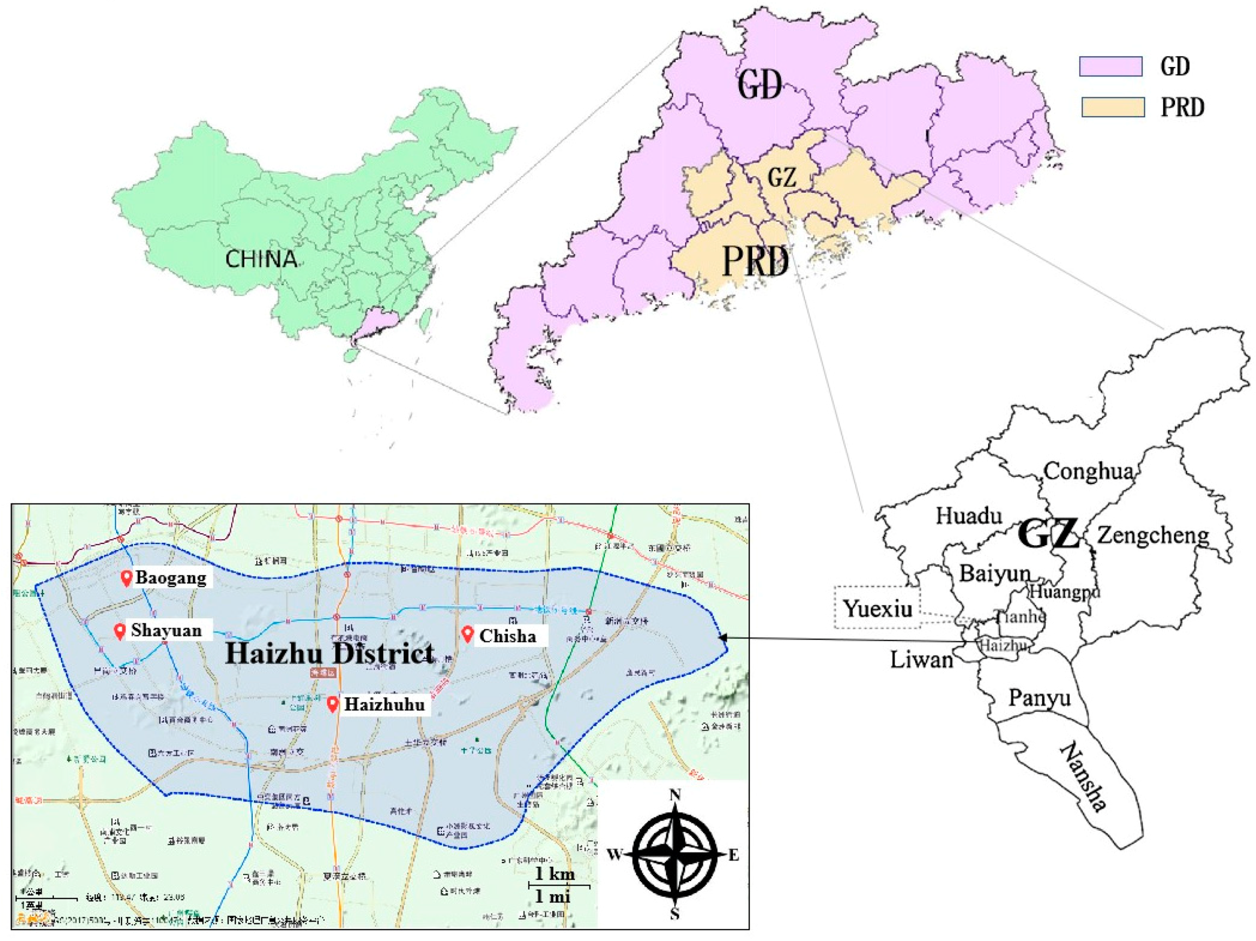
2.1. Observation Data

Air quality monitoring data, including the hourly concentrations of pollutants (CO, SO2, PM2.5, PM10, NO2, O3) and daily AQI (Air Quality Index), were collected from Guangzhou Environmental Monitoring Centre data network (http://210.72.1.216:8080/gzaqi_new/RealTimeDate.html). Hourly and daily meteorological data [wind speed, wind direction, relative humidity (RH), temperature, satellite cloud images, etc.] were downloaded from the Guangzhou meteorological data network (http://data.tqyb.com.cn/weather/index.jsp). These websites are regularly maintained by the government, and the data are released to the public. The data mentioned above were used to analyse the air quality status and pollution episodes in 2015, and to evaluate the WRF-Chem model’s performance.

2.2. Emission Inventory and Scenarios

2.2.1. Emission Inventory

The anthropogenic emissions from the 2012-based Multiresolution Emission Inventory for China (MEIC) [43] (http://www.meicmodel.org/), biogenic emission parameterisation [44], dust emission parameterisation [45], and sea salt emission parameterisation [46], and the marine emission from EDGAR (Emission Database for Global Atmospheric Research, http://edgar.jrc.ec.europa.eu/) were applied in this study. The 2012-based MEIC was a Chinese national emission inventory with a resolution of 0.25° × 0.25° based on 2012 emission status, developed by Tsinghua University. It included the emissions in major sectors, such as transport, industry and human residential, etc. [13]. Previous studies reported that MEIC was well developed by a technology-based emission model [47] and similar emission datasets have been widely used in the numerical simulation for cities in PRD [27,48].
The emissions in the key research area, Guangzhou, were obtained based on the Guangzhou ambient air quality plan (2016–2025) [49]. The emission of air pollutants from different sources in Haizhu district in 2015 was retrieved from the Guangzhou environmental protection bureau’s data network (http://www.gzepb.gov.cn/infoindex.htm). Based on the statistics yearbook (http://210.72.4.52/gzStat1/chaxun/njsj.jsp) and the Guangzhou environmental protection bureau’s data network, the emission inventory was generated according to Chinese national technical guidelines [50,51] and relevant studies (Zheng et al., 2009 [52]; Zhao et al., 2015 [53]). Spatial allocation of emission inventory depended on the source characteristics. Haizhu district is an urban area, and the major emission sectors are industry, residential, and (road) transport. Emission sectors, corresponding inventory technical guidelines, and special allocation rules in this research are shown in Table S1.
According to the 2015-based Haizhu district emission inventory, the 2020 Haizhu district emission inventory was predicted with the extrapolation function [13] [EI_2020 = fx (EI_2015 × activity factor), where EI refers to the emission inventory, and the activity factor refers to the trend of emission sections, gained from emission control policies for the 13th Five-Year period [12,49,54] and the trend of city development in the past five to ten years (e.g., society, economy, vehicle and population, etc.) according to the statistical yearbook network (http://210.72.4.52/gzStat1/chaxun/njsj.jsp)]. We note that the emission inventory in Haizhu district is compiled on an annual resolution. The resolution of these inventories was 0.01° × 0.01°. All of the emission inventories have the same major sectors (transport, industry, and residential, etc.).

2.2.2. Emission Scenarios

Because the major and easily controlled sections had been regulated during the 12th Five-Year Plan period (12th FYP), the 13th FYP emission control policy was set more aggressively: industries generating air pollution will be moved out from the central city area, ultraclean/effective technology will be widely used, the ratio of public transport will rise to 70% of motorised travel [12], electric buses will be applied widely, accounting for 63% of public buses [54], vehicle emission standards and fuel standards will be strengthened (specifically, eliminating high pollution vehicles, implementing the new national emission standard of vehicle and the new national vehicle fuel standard, etc.), and VOC emission will be controlled entirely in particular industries (e.g., chemical industry, paint industry, and printing industry, etc.) [49].
Four scenarios were designed to evaluate the impact of the 13th FYP on the air quality in Haizhu district in 2020. The meteorological conditions were assumed to be unchanged, which means that the meteorological conditions in 2015 were used for all scenarios in 2020. The four 2020 scenarios are as follows (also in Table S2):
Scenario 2020A was proposed such that both Haizhu emission control policy and Guangzhou (except Haizhu) emission control policy would follow the 2015 emission control policy tendency. This scenario is a baseline scenario.
Scenario 2020B was designed such that Haizhu emission control would be implemented based on the 13th FYP emission control plan, while Guangzhou (except Haizhu) would still adhere to the 2015 emission control policy.
Scenario 2020C was a 13th FYP policy scenario in which both Haizhu emission control policy and Guangzhou (except Haizhu) emission control policy would be implemented based on the 13th FYP emission control plan.
Scenario 2020D was a scenario for vehicle control in Haizhu due to the significance of vehicle emission in Haizhu. In this scenario, vehicle control in Haizhu would be implemented based on the 13th FYP emission control plan, while other emission source controls in the Haizhu and Guangzhou (except Haizhu) emission control policy would remain as the 2015 emission control policy tendency. We note that the contribution of vehicle emission in Haizhu district is <10% of that in Guangzhou city.
Table 1 shows the changes in emissions of SO2, NOx, CO, PM10, PM2.5, and VOCs for the different scenarios in the whole city of Guangzhou. The 2020A, 2020B, and 2020D scenario emissions would be higher than the 2015 emissions (SO2, NOx, CO, PM10, PM2.5, and VOCs would increase 57.2–58.9%, 47.4–48.6%, 60.1–60.2%, 14.6–15.1%,25.8–26.4%, and 24.9–25.0%, respectively), whereas the 2020C scenario emission would be lower than or roughly equal to the 2015 emission. The difference of emissions among each scenarios indicates that the emission control of the whole Guangzhou city would significantly affect the 2020 emission. Additionally, the emission ratio (VOCs/NOx) would be around 0.72 in scenarios 2020A, 2020B, and 2020D and 0.60 in scenario 2020C, lower than 0.86 in 2015.
The changes in emissions for each sector are shown in Figure 2. SO2 emission from the sectors residential, vehicle, and others, and NOx emission from the residential sector in the four 2020 scenarios would be lower than those in the 2015 emission. PM2.5 emission and PM10 emission from the residential sector in scenarios 2020B and 2020C would also be lower than those in the 2015 emission. In scenarios 2020C, NOx emission from the vehicle and others sectors, CO emission from the industry, residential, and vehicle sectors, and VOCs emission from the residential sector would be higher than those in the 2015 emission. Overall pollutants emissions in scenarios 2020A, 2020B and 2020D would be higher than those in 2015, pollutants emissions in scenarios 2020C would be lower than in 2015, except that CO emission in scenarios 2020C would be slightly higher than that in 2015.

2.3. WRF-Chem Model Setup

2.3.1. Description of WRF-Chem Model

WRF-Chem is a chemical transport model developed by the community led by NOAA/ESRL (Earth System Research Laboratory, The United States National Oceanic and Atmospheric Administration) [55,56], and it is widely used for analysing heavy pollution processes and the effectiveness of emission control measures [22,27,57].

2.3.2. Configuration of WRF-Chem

In this study, a three-nested domain was applied for model set-up (Figure S2), with grid cell areas of 9 × 9 km, 3 × 3 km, and 1 × 1 km, respectively. The biggest domain covered the southern China area, the middle domain covered PRD, and the smallest one covered the Guangzhou central area. There were 27 sigma levels for all domains, and in this study, the data of the ground level was mainly used. The NCEP (the United States’ National Centers for Environmental Prediction) 6-h FNL (Final Operational Global Analysis data) meteorological data and the emission inventory mentioned above were input for model setup. The simulation data from MOZART (Model for Ozone and Related Chemical Tracers, https://www.acom.ucar.edu/wrf-chem/mozart.shtml) was used as the initial and boundary chemistry data [58]. The related parameterisation schemes in the simulation were the Regional Acid Deposition Model, version 2 (RADM2) gas-phase chemical mechanism [59] and the MADE/SORGAM (Modal Aerosol Dynamics Model for Europe/Secondary Organic Aerosol Model) aerosol chemical mechanism [60,61]. We have not activated the feedback from chemistry on meteorology. The first 120 h in the simulation were used as the model spin-up.

2.3.3. Cases Setup

(1) Evaluation of overall air quality in 2020
The month of October was used as a proxy of the entire year of 2015 since the pollutant concentrations in October 2015 were very similar to those in the whole year (details are shown in Section 3.1). WRF-Chem simulations were conducted with the emissions in four 2020 scenarios and the emissions in 2015. The simulated concentrations of PM2.5, PM10, SO2, NO2, CO, and O3 were compared between results of the four 2020 scenarios and the result of 2015, in order to evaluate the effectiveness of the 13th FYP policy on air quality. The meteorological conditions for 2020 scenarios were assumed to be the same as the meteorological conditions in 2015. The results are shown in Section 3.3.
(2) Evaluation of air quality during pollution episodes
To identify the air quality status, we analysed the annual air quality situation and air pollution events based on the data observed in four urban stations (Baogang, Chisha, Shayuan, and Haizhuhu) in Guangzhou Haizhu district (Figure 1). A pollution episode was defined as a short period consisting of subsequent days (at least one day) with the AQI ≥ 101 [62]. A heavy pollution episode was a pollution episode with AQI ≥ 201 [62].
The pollution episodes in 2015 are shown in Table 2 (more information is shown in Table S3). The table shows that the number and the pollution level of pollution episodes had seasonal characters. The pollution episodes occurred more often in winter, and heavy pollution was observed in the summer and winter. The Shayuan station and Haizhuhu station suffered pollution episodes more than other stations in 2015, and Shayuan was the only station where the heavy pollution episodes were observed in both winter and summer (14–28 January 2015, and 3–8 August 2015, respectively). The two heavy pollution episodes were typical pollution (PM2.5 and NO2 pollution in winter, O3 pollution in summer [63]). Therefore, the two heavy pollution episodes in Shayuan were analysed with pollution and meteorology progress (results shown in Section 3.1.2). Also, the meteorology conditions of these two episodes were applied in the 2020 scenarios numerical simulations with WRF-Chem to evaluate the effectiveness of the 13th FYP policy on air quality of pollution episodes (specifically, PM2.5 and NO2 pollution for the winter episode, O3 pollution for the summer episode). The simulation results are shown in Section 3.4.

3. Results and Discussion

3.1. Air Quality in Haizhu in 2015

3.1.1. Overview

The annually-averaged concentrations of PM2.5, PM10, SO2, and NO2 were 40 μg/m3, 61 μg/m3, 14 μg/m3, and 49 μg/m3, respectively, in Haizhu district in 2015, which were higher than those in the whole of Guangzhou city (39 μg/m3, 59 μg/m3, 13 μg/m3, and 47 μg/m3, respectively [64]). The 95th percentile of the CO daily concentration was 0.9 mg/m3, in Haizhu district in 2015, which was lower than that in the whole of Guangzhou city (1.5 mg/m3, [64]), The routine pollutants (except for O3) peaked in January (winter), among which PM2.5 and NO2 were the major pollutants. The 90th percentile of the daily 8 h maximum O3 concentration (O3-8h) in 2015 was 139 μg/m3, slightly lower than that in Guangzhou (145 μg/m3; [64]). O3-8h peaked in September (summer to autumn, or hot season). O3 was also the key pollutant in summer and autumn in Haizhu district [64]. These observational results suggested that air quality in Haizhu was still harmful to human health (the thresholds: PM2.5 ≤ 10 μg/m3 annual mean, PM10 ≤ 20 μg/m3 annual mean, NO2 ≤ 40 μg/m3 annual mean, O3-8h ≤ 100 μg/m3 8 h mean) [65] and it was worse than the Guangzhou average level in 2015, which highlights the necessity of district/town regulation in air quality control. Please note that this study does not intend to estimate the influence of air quality on human health which is sensitive to the exposure levels (the levels of air pollutants). The pollutant concentrations in October 2015 were very similar to those in the year of 2015 (a-SO2, a-NO2, a-PM10, a-PM2.5, a-O3-8h, a-CO, in Figure 3a).
Compared with the 13th FYP targets in 2020 (PM2.5 ≤ 30 μg/m3, PM10 ≤ 50 μg/m3, SO2 ≤15 μg/m3, NO2 ≤ 40 μg/m3, O3-8h ≤ 160 μg/m3, and CO ≤ 2 mg/m3) in Guangzhou [49] (Figure 3b), PM2.5, PM10, and NO2 concentrations in 2015 exceeded the targets, and the air pollutant emission could even rise in the coming years (Table 1). Haizhu district could face worsening air quality, and more emphasis should be placed on the control measures and effectiveness assessment for PM2.5 and NO2 during the 13th FYP so that the measures can be duly adjusted to achieve the 13th FYP targets.

3.1.2. Air Quality during Pollution Episodes

Table 2 summarizes the pollution episodes in Haizhu district in 2015. Shayuan station was the only station where heavy pollution episodes were observed in both winter and summer, and the two pollution episodes were also the typical pollution (PM2.5 and NO2 pollution in winter, O3 pollution in summer). Therefore, these two typical pollution episodes in Shayuan will be analysed in detail below.
(1) Heavy pollution episode in winter
A winter heavy pollution episode in Haizhu district occurred during 14–28 January 2015 (Table S4 shows the statistical data). In this pollution episode, the air quality was light pollution in the beginning (15–19 January), then the pollution level peaked during 20–21 January. It finally decreased to light pollution again in the third period (22–27 January). On 28 January, the air quality was good again. This episode was a process in which the air quality decreased gradually and then increased gradually. During this episode, the wind speed was in the range of 1.1–2.9 m/s, the RH was in the range of 52–85%, and there was no precipitation. The temperature was in the range of 10.3–18.0 °C, and the surface pressure was in the range of 1009.1–1016.1 hPa. The low wind speed during this winter episode (~1.5 m/s) indicated that the atmosphere was stable, and as reported in previous studies, low or calm wind speed generally leads to high pollution [67,68], because stable atmospheric condition favours the accumulation of pollutants. There is another possibility that the existence of temperature inversion layer could also lead to the accumulation of the air pollutants (e.g., Malek et al., 2006 [69]).
(2) Heavy pollution episode in summer
A summer heavy pollution episode in Haizhu district happened during 3–8 August 2015 (Table S5). The whole episode covered only six days, including the two days of light pollution (4 and 7 August), one day of moderate pollution (5 August), and one day of heavy pollution (6 August). The pollution occurred and disappeared within a short time, but it exhibited high intensity. In this episode, the wind speed was in the range of 1.1–4.4 m/s, the RH was between 65 and 76%, and there was no precipitation. In the first period (3–6 August 2015), the wind speed was in the range of 1.1–1.4 m/s. There was no precipitation nor cloud. The temperature was in the range of 27.6–30.3 °C, and the surface pressure was in the range of 991.7–1002.4 hPa. The hourly temperatures were between 23.4 and 35.6 °C. Sunny weather, low wind, and high temperatures would create favourable conditions for O3 production and accumulation [10]. Then, the wind speed increased to 3.9–4.4 m/s during 7–8 August 2015. Strong wind transported the air pollutants out of Haizhu, improving the air quality in Haizhu to light pollution. The temperature inversion layer might also enhance the accumulation of the air pollutants (e.g., Malek et al., 2006 [69]).

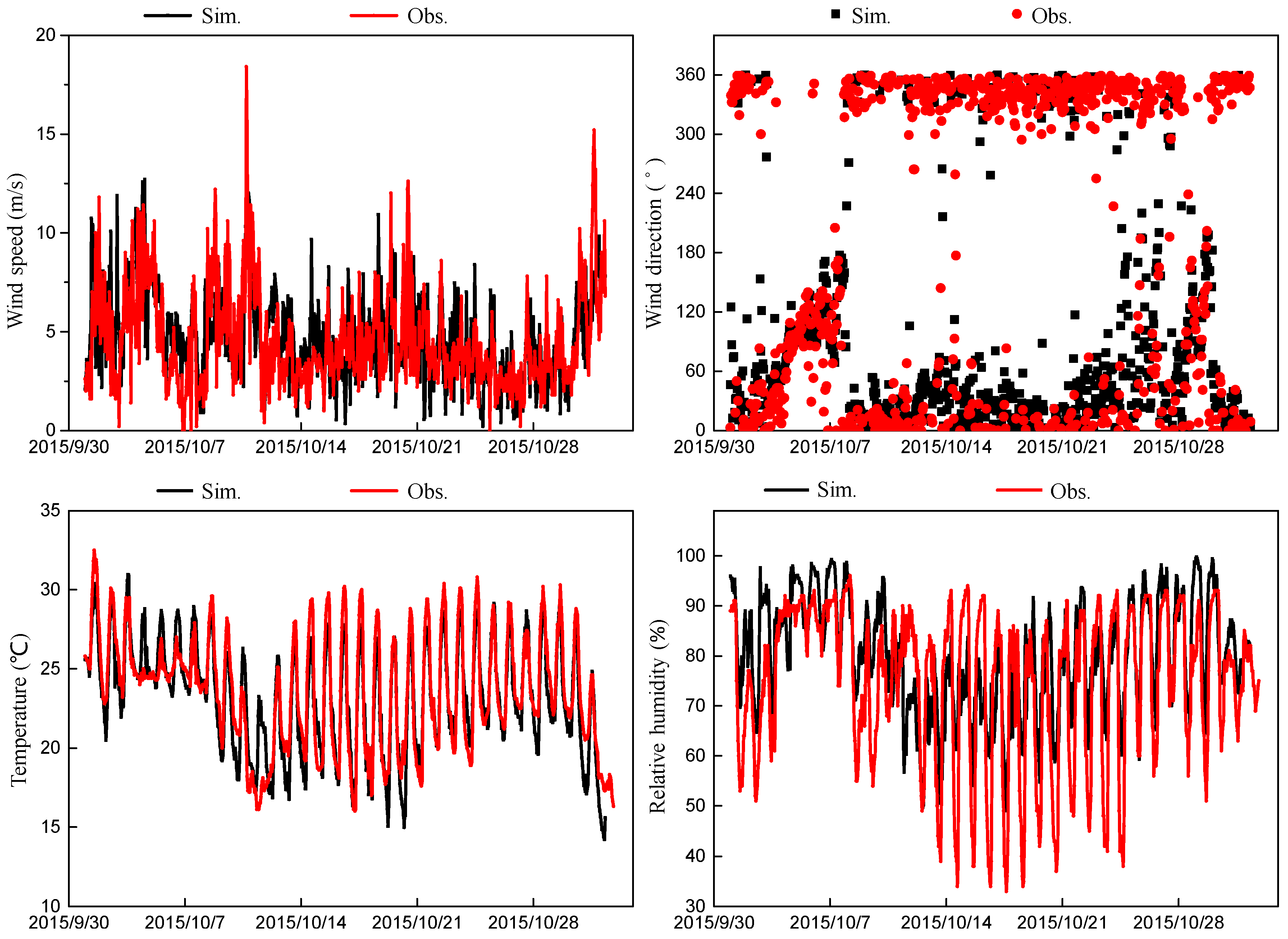
3.2. Evaluation of WRF-Chem Model Performance

October was the month when the concentrations of PM2.5, NO2 and O3 (the major pollutants in Haizhu) were all at elevated levels. Therefore, we used the observed data in October to evaluate the performance of the WRF-Chem simulation.
(1) Meteorological simulation evaluation
The simulated surface meteorological parameters (wind speed, wind direction, temperature, and RH) in Guangzhou were validated with the observed data (Table S6 and Figure 4). The temperature, RH, and wind speed in the simulation were generally in line with the observations (Table S6), and the simulated wind directions covered the observed wind directions (Figure 4, wind direction). Similar model behaviour was reported in some previous studies [9,70,71]. The over-prediction of the wind speed in the present study is probably due to the underestimation of the roughness in the cities. For example, the constructions in the urban area are not adequately represented in our model simulation although a very fine resolution of 1 km is already used. Overall, the simulation generally reproduced the meteorological condition in 2015.
(2) Chemical simulation evaluation.
Simulated pollutant concentrations were also compared to observed data, including O3 daily 8 h maximum concentration and other pollutants’ daily-averaged concentrations (CO, PM2.5, PM10, SO2, and NO2). Metrics of evaluation on model performance are shown in Table S7. The ranges of the mean-bias (MB) and root-mean-square-error (RMSE) on pollutant concentrations were −8.07 μg/m3 to 24.34 μg/m3, 9.81 μg/m3 to 48.35 μg/m3, respectively, except CO. The MB and RMSE of CO were −0.32 mg/m3 and 0.43 mg/m3, respectively. Compared to previous studies [13,70,71,72], the model in this paper showed similar behaviour. Figure 5 shows that the general characteristics of the routine pollutants were captured by the simulation. Monthly averaged simulated concentrations of NO2, PM10, SO2, CO, O3-8h, and PM2.5 at the locations of the monitoring sites were 147.6%, 101.1%, 112.0%, 65.1%, 91.4%, and 80.9% of the observations, respectively. Concentrations of NO2, PM10, and SO2 were overpredicted in the simulation, and concentrations of CO, O3-8h, and PM2.5 were underestimated. It is noticeable that there was an observed peak in pollution on 14 October which was underestimated in the simulation. Concentrations of NO2, PM10, SO2, CO, O3-8h, and PM2.5 in the simulation were 39%, 49%, 42%, 52%, 49%, and 65% less than that of the observation on 14 October, respectively. The most probable reason for the discrepancy is the meteorological condition was not well captured. Other possible causes include the uncertainty of the emission inventory, the uncertainty of the chemical scheme in simulating the formation of secondary air pollutants, etc. The uncertainty of emission inventories results from the uncertainty in the activity level, the emission factor, and the different grid size [73,74,75]. The simulation of secondary air pollutants (O3, secondary inorganic and organic aerosol) is a hot research topic and still contains some uncertainty as reported in Ahmadov et al. (2012) [76], Li et al., (2018) [77], etc. Besides, the planetary boundary (PBL) scheme also plays an important role in predicting the level of air pollutants at the surface and the reader is referred to relevant studies (e.g., Banks and Baldasano, 2016 [78]; Shin and Hong, 2011 [79]; Hu et al., 2010 [80]) for the evaluation of various PBL schemes including the one used in the present study, i.e., the YSU (Yonsei University) scheme [81]. There is also the possibility that the representative area of the measurement site differs from the grid cell that contains the site and such difference might lead to the difficulty of directly comparing the simulation with observation (e.g., Schutgens et al. 2016 [82]).
In the present study, we follow the relevant air quality modelling studies, e.g., those studies included in Table S7, to use the statistic tools to evaluate the WRF-Chem model performance. While the statistic method can provide some insights into the model abilities, it would help if some advanced diagnostic tools, e.g., the simulation error apportioning techniques proposed by Solazzo et al. (2017a) [83] and Solazzo et al. (2017b) [84], are adopted in future study to identify the critical processes that demand most urgent attention.

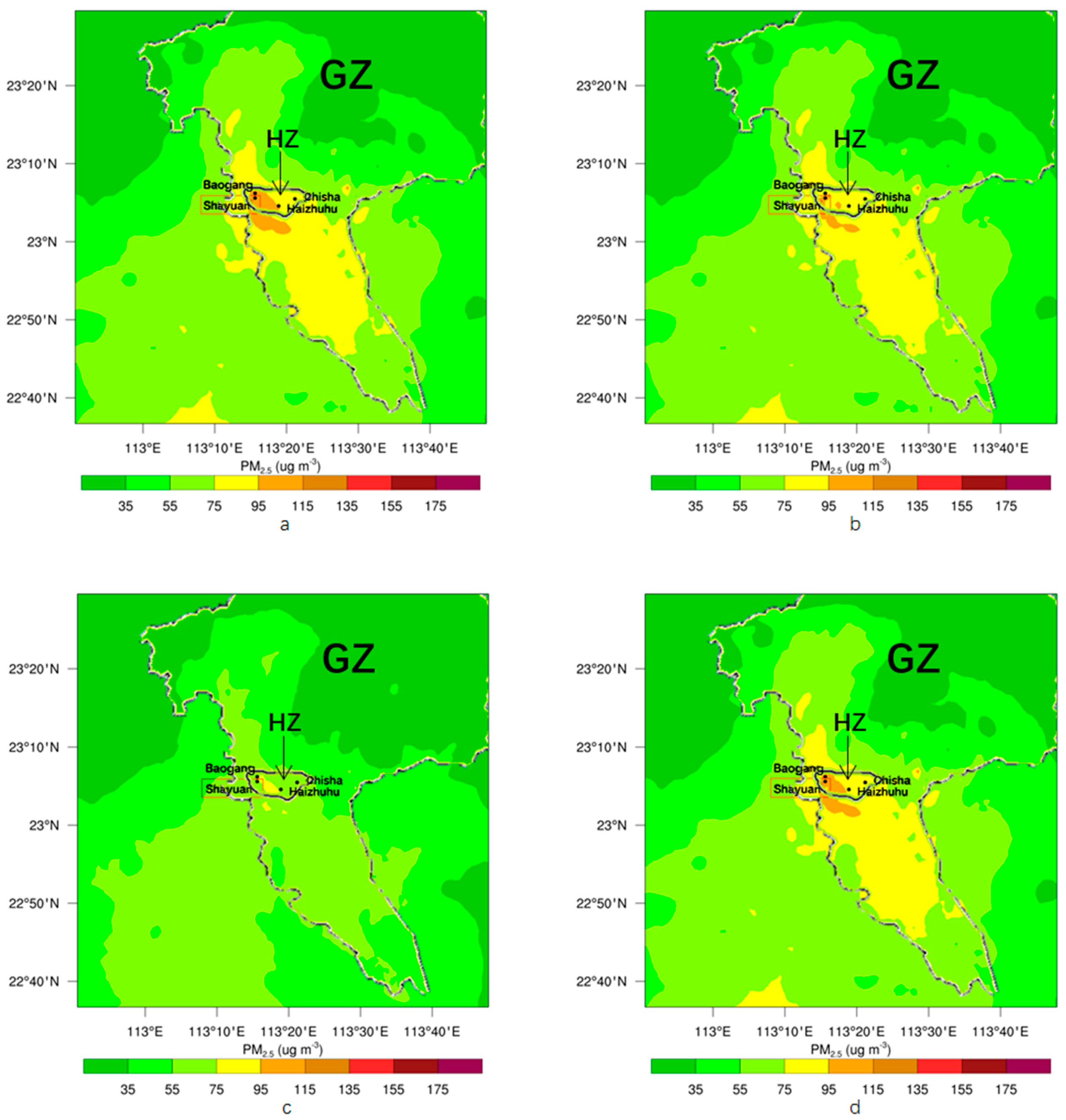
3.3. Effect of 13th FYP on Overall Air Quality in Haizhu in 2020

Since the pollutant concentrations in October 2015 were very similar to those in the whole year, the simulated results in the four 2020 scenarios in October are used for evaluating the effect of the 13th FYP on the air quality in Haizhu by comparing to the simulation for October 2015 (Figure 6).
Figure 6 shows that simulated concentrations of five pollutant species (CO, NO2, PM2.5, PM10, and SO2) in scenario 2020C are lower than pollutants concentrations simulated in 2015. For O3, 2020 scenarios’ simulation results are higher than 2015 result. CO, PM2.5, PM10, and SO2 concentrations in 2020 scenarios A, B, D are higher than the pollutants concentration in 2015 simulation. NO2 concentrations in the four 2020 scenarios are slightly lower than the concentration in 2015 simulation.
It is noticeable that O3 concentrations in all of the four 2020 scenarios are higher than those in 2015 simulation, which means that ozone pollution will probably get worse by the end of 13th FYP. Although scenario 2020A had the slightly less pollution than other scenarios had, the level of Ox (O3 + NO2) in scenario 2020A was higher than that of other scenarios (Figure 6), which means that atmospheric oxidation in scenario 2020A was more elevated [13,85]. It would cause the more intensive formation of secondary aerosols, which would lead to regional pollution [86]. Meanwhile, the level of Ox in scenario 2020C was the lowest.
In Section 3.1, the observed concentrations of PM2.5, PM10, and NO2 in 2015 exceeded the targets. Meanwhile, the WRF-Chem simulations suggested that from 2015 to 2020, the concentrations of PM2.5 and PM10 would increase in scenarios 2020A, 2020B, and 2020D. Therefore, the real concentrations of aerosols in 2020 could be higher than those in 2015 and further exceed the targets. The observed O3-8h concentration in 2015 did not exceed the target (Section 3.1), but with the increasing trend from 2015 to 2020 as simulated in all scenarios, the real O3-8h concentration in 2020 should be considered as a cause for concern.
According to the simulations, by the end of 13th FYP, if the emission control policy just follows 12th FYP policy (scenario 2020A), the air pollution would increase and the control on all emission sectors in Haizhu (scenario 2020B) and control just on vehicle emissions in Haizhu (scenario 2020D) would have a similar impact on air quality, and could not improve air quality very much. The scenario 2020C (the comprehensive emission control measures taken in the whole Guangzhou city) would have the better effect on the emission control than other scenarios would do. Among the four 2020 scenarios, the scenario 2020C is the better scenario.
According to Figure 6, pollutant concentrations between scenario 2020B and 2020D are similar. The effect of controlling every emission sectors in Haizhu district would be almost equal with the effect of only controlling the traffic emission in Haizhu district, suggesting that traffic source would be a key source in Haizhu district.
Wang et al. (2016) [13] used WRF-CMAQ model (a base case in 2010, two cases in 2020) and evaluated the impact of emission control measures on the air quality in the PRD region, and their results showed that reducing NOx emissions would cause rising PM2.5 levels in certain areas, although it would benefit with reduction of regional PM2.5. They also noted that O3 formation in PRD was generally VOCs-limited and cutting VOCs emission could benefit the reduction of overall O3. Liu et al. (2017) [14] assessed the influence of vehicle emission control measures for 2015–2020 in the PRD region on air quality and climate and their results suggested that, if vehicle emission wasn’t controlled, most air pollutants and GHG would increase by 20–64% by 2020.

3.4. Effect of 13th FYP on Air Quality during Heavy Pollution Episodes in Haizhu in 2020

To evaluate the effect of 13th FYP on NO2 and PM2.5 in the winter heavy pollution episode and O3 in the summer heavy pollution episode, we conducted the WRF-Chem simulations with the four 2020 pollution control scenarios (2020A, 2020B, 2020C, and 2020D). Table 3 shows the changes in pollutant concentrations of the four scenarios. Since Table 3 has summarized the overall impacts (in numbers) of each emission reduction scenarios on the concentration of PM2.5, NO2, and O3, we will present the spatial variation of the impact in Figure 7, Figure 8 and Figure 9 in the following text. According to the results of Section 3.2, the simulation during the observational peak was underestimated compared to the measurement, implying that the actual concentrations of pollutants in 2020 could be higher than our simulations.
(1) Effect on PM2.5 and NO2 in winter heavy pollution episode
For the simulated concentrations of PM2.5 and NO2 in Shayuan station, the concentrations of PM2.5 and NO2 were in the order of 2020A > 2020D > 2020B > 2020C. Comprehensive emission control measures taken in the whole of Guangzhou (2020C) would be able to reduce concentrations of PM2.5 and NO2 two times more than those just in Haizhu (2020B). In previous research, emission control from outside of Beijing contributed 8–14% to the improvement of the air quality in Beijing during APEC [57]. Therefore, regional control policies are needed. Regional control measures in a whole city could affect the air quality of the urban district, even if the district is just an isolated island. Referring to the measures in Haizhu, the effect of vehicle emission control (2020D) on PM2.5 (NO2) reduction would be ~44% (~71%) of the effect of comprehensive measures (2020B), meaning that vehicles are the major PM2.5 (NO2) emission source in Haizhu. Vehicle emission is a typical problem in urban areas of China [87]. Previous studies showed that vehicle emission accounted for 21%, 10%, and 19.3% of the total PM2.5 in Dongguan (2014) [68], Guangzhou (2014) [88], and PRD (2012) [89], respectively.
In the worst meteorological condition, PM2.5 pollution on Haizhu district would be improved, as shown in Figure 7c and Figure 7b, which means that the effects on regional air quality of scenarios 2020C and 2020B were relatively significant. In particular, compared with 2020D (Figure 7d), the improvement on regional air quality in 2020B was more obvious, although the PM2.5 pollution in the particular station (Shayuan) seemed to have no significant difference. In Figure 8, NO2 pollution shows a similar situation. It indicates that regional and comprehensive measures could improve regional air quality during heavy pollution days.
(2) Effect on O3 in summer heavy pollution episode
For the Shayuan station, the O3 pollution in scenario 2020B would be higher than in other scenarios, and the O3 pollution in the other scenarios were in the order 2020C > 2020D > 2020A (Table 3). The simulation results suggested that the O3 level increases from 2015 to 2020 in all emission scenarios even in 2020C in which the rest of air pollutants decrease. Such changes of O3 concentration is probably because the Haizhu district is a VOC-limited region in which the O3 level increases (decreases) with the reduction of NOx (VOCs) emission (e.g., Sillman, 1999 [90]). There are generally two pathways that can be adopted to relieve the O3 pollution in VOC-limited region like Haizhu district. (1) To significantly reduce the NOx level and push the Haizhu district into NOx-limited region in which O3 level decreases with the reduction of NOx and VOCs. However, in this pathway, there will be a period in which O3 level significantly increases before it starts to decrease. (2) To adopt a proper reduction ratio of VOCs/NOx and flatten the O3 increase to the largest extent during the transient from VOC-limited region to NOx-limited region. But this pathway requires a great deal of effort to determine a favourable reduction ratio of VOCs/NOx and cut the emission of VOCs from various sectors.
The findings in the present study highlight the complexity and nonlinear chemistry of O3 formation and call for further investigations. For example, the reduction ratio of VOCs/NOx for anthropogenic sources was generally suggested to be 1:2 in PRD [10]. However, considering the change of precursor emissions and meteorological conditions, the ratio of VOCs/NOx might need to be further studied. Besides, the NO2 is overpredicted in the present study implying that the VOC-limited nature in Haizhu district might be overpredicted, although there is very low chance that Haizhu district is a NOx-limited region in 2015 because the NOx is still at an elevated level and this region (PRD) has been repeatedly diagnosed as a VOC-limited region (e.g., Xue et al., 2014 [91]). Moreover, the formation of O3 depends on the local mixture of NOx and VOCs. Therefore, the location/sector of the emission of NOx and VOC, apart from the overall reduction of NOx and VOC in an area, might have an impact on the changes of O3. Although we have made some effort on such topic by evaluating the effect of only controlling traffic emission on air quality (scenario 2020D), it would be of interest to adopt more sophisticated tools, e.g., a tagging technique (Grewe, 2013 [92]), to evaluate the effect of various combinations of emission reduction in sectors in future study.
The simulated O3-8h distribution on 6 August is shown in Figure 9 to demonstrate the difference of regional O3 pollution in Haizhu district. Ozone pollution would be relieved in scenario 2020C (Figure 9c) compared with that in other scenarios (Figure 9a,b,d). It is noticeable that ozone pollution in the southwest area (red area, suburban and rural area) in 2020C (Figure 9c) could be smaller than those in other scenarios (Figure 9a,b,d), which may be because of the suitable ratio of precursors in that area of scenario 2020C, although the pollution in Haizhu (urban area) seemed to have no significant difference. The difference of regional O3 pollution shows that in the southwest area (suburban and rural area), the policy in scenario 2020C could decrease the O3 significantly (less red area), and in other regions, e.g., in Haizhu (urban area), the effect is less noticeable, which indicated that the control of ozone pollution should be taken according to local conditions, i.e., measures in urban areas should be different from those in rural areas. We note that transboundary transport of O3 and its precursors (CO, VOCs, and NOx) due to mesoscale dynamics complicates O3 pollution control and requires strong and efficient cooperation among the adjacent regions.

4. Conclusions

In this study, the air quality in the year of 2015 and during pollution episodes in Haizhu district were analysed, and the impacts of emission control scenarios by the year of 2020 on air quality were evaluated using the WRF-Chem numerical simulation.
For the air quality in Haizhu 2015, the annually-averaged concentrations of PM2.5, PM10, SO2, and NO2 were higher than those in the entire Guangzhou city. O3-8h was slightly lower than that in Guangzhou. Pollution episodes in Haizhu in 2015 primarily occurred in summer and winter. The typical winter pollution episode (14 to 28 January) was a process of gradual accumulation of pollution and dissipation, with NO2 or PM2.5 as the key pollutants, associated with the wind. The heavy pollution episode in the hot season (3 to 8 August) was a process of pollution that occurred and disappeared quickly, with O3 as the key pollutant, due to suitable local pollution and strong sunshine.
The WRF-Chem simulation generally captured the observed chemical characteristics, suggesting that the WRF-Chem model could be used to simulate air quality in the research case.
Emission control scenario 2020C (comprehensive measures taken in the whole of Guangzhou city) would improve air quality more significantly than other scenarios (measures taken in Haizhu) under all conditions (heavy pollution conditions and annual level). For urban areas, scenario 2020D (vehicle emission control) would account for more than half of the influence of 2020B (all source emission controls) on air quality. By the end of the 13th FYP, it is noticeable that O3 pollution would increase, which indicates that the control ratio of VOCs and NOx may be unfavourable and requires further assessment. It would be of interest to perform simulations with the meteorology/chemistry interactions to investigate the influence of policies on O3 and other air pollutants in future research.
Our study suggested that control measures should be strengthened for NO2, PM2.5, and PM10, and control ratio of VOCs and NOx should be adjusted for controlling O3. The urban area should focus on vehicle emission control, strengthen regional cooperation on pollution control, and establish short-term measures for heavy pollution conditions.

Supplementary Materials

The following are available online at https://www.mdpi.com/2076-3417/10/15/5276/s1, Figure S1: Research framework, Figure S2: WRF-Chem simulation domain, Table S1: Emission sectors, corresponding inventory technical guidelines and special allocation rules, Table S2: Description of emission control scenarios, Table S3: Detailed information for pollution episodes observed in Haizhu monitoring stations, 2015, Table S4: Statistical data for heavy pollution episode in Haizhu district during 14–28 January 2015, Table S5: Statistical data for heavy pollution episode in Haizhu district during 3–8 August 2015, Table S6: Performance statistics for meteorological simulation ( hourly statistical data in October 2015), Table S7: Statistical comparison of model evaluation in this paper and previous study.

Author Contributions

J.Z. and H.D. designed the study. Y.L. and C.F. collected and analysed data. T.G. and L.L. did emission data preparation and generated the figures. R.O. and M.W. did the policy investigation. J.Z. contributed to literature search, numerical simulation and writing the manuscript. All authors have read and agreed to the published version of the manuscript.

Funding

This research was funded by the National Key Research Program (No. 2016YFC0202005), the Natural Science Foundation of China (No. 41975165; No. 11802347), the Fundamental Research Funds for the Central Universities (No. 20lgpy180), and the social science and technology development (key) project of Dongguan city (No. 2019507101161). The APC was funded by the National Key Research Program (No. 2016YFC0202005).

Acknowledgments

The author greatly appreciated Guangzhou Haizhu District Environmental Monitoring Station for providing the data in this work and Tsinghua University for providing MEIC. Thanks also go to Qinyi Li in Spanish National Research Council and Jinpu Zhang in Guangzhou Environmental Monitoring Center for valuable suggestions and fruitful discussion.

Conflicts of Interest

The authors declare no conflict of interest.

References

  1. Gulia, S.; Shiva, N.S.M.; Khare, M.; Khanna, I. Urban air quality management—A review. Atmos. Pollut. Res. 2015, 6, 286–304. [Google Scholar] [CrossRef] [Green Version]
  2. SC (State Council of People’s Republic of China. Air Pollution Control Action Plan. 2013. Available online: http://www.gov.cn/zwgk/2013-09/12/content_2486773.htm (accessed on 23 November 2018).
  3. CAA (Clean Air Asia). China Air 2015—Air Pollution Prevention and Control Progress in Chinese Cities. 2015. Available online: http://cleanairasia.org/wp-content/uploads/2016/03/ChinaAir2015-report.pdf (accessed on 23 November 2018).
  4. CAA (Clean Air Asia). China Air 2016—Air Pollution Prevention and Control Progress in Chinese Cities. 2016. Available online: http://www.allaboutair.cn/a/cbw/bg/2016/0822/472.html (accessed on 23 November 2018).
  5. BJMBEE (Beijing Municipal Bureau of Ecoloy and Environment). Beijing Environmental Statement 2015. 2015. Available online: http://www.bjepb.gov.cn/bjhrb/xxgk/ywdt/hjzlzk/hjzkgb65/index.html (accessed on 23 November 2018).
  6. SHEP (Shanghai Environmental Protection). Shanghai Air Quality Report. 2015. Available online: http://www.sepb.gov.cn/hb/fa/cms/shhj/list_login.jsp?channelId=5157 (accessed on 23 November 2018).
  7. Zhan, J.; Liu, Y.; Lin, L.; Ding, H.; Xu, W. Investigation of spatial and temporal association of PM2.5 pollution during the winter of 2014 in typical cities of Pearl River Delta. Res. Environ. Sci. 2017, 30, 110–120. [Google Scholar] [CrossRef]
  8. Ma, X.; Jia, H. Particulate matter and gaseous pollutions in three megacities over China: Situation and implication. Atmos. Environ. 2016, 140, 476–494. [Google Scholar] [CrossRef]
  9. Li, M.; Song, Y.; Mao, Z.; Liu, M.; Huang, X. Impacts of thermal circulations induced by urbanization on ozone formation in the Pearl River Delta region, China. Atmos. Environ. 2016, 127, 382–392. [Google Scholar] [CrossRef]
  10. Wang, T.; Xue, L.; Brimblecombe, P.; Lam, Y.F.; Li, L.; Zhang, L. Ozone pollution in China: A review of concentrations, meteorological influences, chemical precursors, and effects. Sci. Total Environ. 2017, 575, 1582–1596. [Google Scholar] [CrossRef]
  11. SC (State Council of People’s Republic of China). Environmental Protection 13th Five-Year Plan. 2016. Available online: http://www.gov.cn/zhengce/content/2016-12/05/content_5143290.htm (accessed on 23 November 2018).
  12. PGGZ (People’s Government of Guangzhou). Guangzhou Environmental Protection 13th Five-Year Plan. 2016. Available online: http://www.gz.gov.cn/gzgov/s2812/201612/467e946dfcb048c0a7bff56655808c60.shtml (accessed on 23 November 2018).
  13. Wang, N.; Lyu, X.P.; Deng, X.J.; Guo, H.; Deng, T.; Li, Y.; Yin, C.Q.; Li, F.; Wang, S.Q. Assessment of regional air quality resulting from emission control in the Pearl River Delta region, southern China. Sci. Total Environ. 2016, 573, 1554–1565. [Google Scholar] [CrossRef]
  14. Liu, Y.H.; Liao, W.Y.; Lin, X.F.; Li, L.; Zeng, X.L. Assessment of Co-benefits of vehicle emission reduction measures for 2015–2020 in the Pearl River Delta region, China. Environ. Pollut. 2017, 223, 62–72. [Google Scholar] [CrossRef]
  15. Maji, K.J.; Dikshit, A.K.; Arora, M.; Deshpande, A. Estimating premature mortality attributable to PM2.5 exposure and benefit of air pollution control policies in China for 2020. Sci. Total Environ. 2018, 612, 683–693. [Google Scholar] [CrossRef]
  16. Yang, X.; Teng, F. The air quality co-benefit of coal control strategy in China. Resour. Conserv. Recycl. 2016, 129, 373–382. [Google Scholar] [CrossRef]
  17. Wang, Z.; Pan, L.; Li, Y.; Zhang, D.; Ma, J.; Sun, F.; Xu, W.; Wang, X. Assessment of air quality benefits from the national pollution control policy of thermal power plants in China: A numerical simulation. Atmos. Environ. 2015, 106, 288–304. [Google Scholar] [CrossRef]
  18. Qiu, X.; Duan, L.; Cai, S.; Yu, Q.; Wang, S.; Chai, F.; Gao, J.; Li, Y.; Xu, Z. Effect of current emission abatement strategies on air quality improvement in China: A case study of Baotou, a typical industrial city in Inner Mongolia. J. Environ. Sci. 2017, 57, 383–390. [Google Scholar] [CrossRef] [PubMed]
  19. Cai, S.; Wang, Y.; Zhao, B.; Wang, S.; Chang, X.; Hao, J. The impact of the “air pollution prevention and control action plan” on PM2. 5 concentrations in jing-jin-ji region during 2012–2020. Sci. Total Environ. 2017, 580, 197–209. [Google Scholar] [CrossRef] [PubMed]
  20. Li, M.; Patiño-Echeverri, D. Estimating benefits and costs of policies proposed in the 13th FYP to improve energy efficiency and reduce air emissions of China’s electric power sector. Energy Policy 2017, 111, 222–234. [Google Scholar] [CrossRef]
  21. Wei, W.; Li, P.; Wang, H.; Song, M. Quantifying the effects of air pollution control policies: A case of Shanxi province in China. Atmos. Pollut. Res. 2017, 9, 429–438. [Google Scholar] [CrossRef]
  22. Guo, J.; He, J.; Liu, H.; Miao, Y.; Liu, H.; Zhai, P. Impact of various emission control schemes on air quality using WRF-Chem during APEC China 2014. Atmos. Environ. 2016, 140, 311–319. [Google Scholar] [CrossRef]
  23. Xu, H.M.; Tao, J.; Ho, S.S.H.; Ho, K.F.; Cao, J.J.; Li, N.; Chow, J.C.; Wang, G.H.; Han, Y.M.; Zhang, R.J.; et al. Characteristics of fine particulate non-polar organic compounds in Guangzhou during the 16th Asian Games: Effectiveness of air pollution controls. Atmos. Environ. 2013, 76, 94–101. [Google Scholar] [CrossRef]
  24. Shen, X.J.; Sun, J.Y.; Zhang, X.Y.; Zhang, Y.M.; Zhang, L.; Fan, R.X.; Zhang, Z.X.; Zhang, X.L.; Zhou, H.G.; Zhou, L.Y.; et al. The influence of emission control on particle number size distribution and new particle formation during China’s V-Day parade in 2015. Sci. Total Environ. 2016, 573, 409–419. [Google Scholar] [CrossRef]
  25. Tan, J.H.; Duan, J.C.; Chen, D.H.; Wang, X.H.; Guo, S.J.; Bi, X.H.; Sheng, G.Y.; He, K.B.; Fu, J.M. Chemical characteristics of haze during summer and winter in Guangzhou. Atmos. Res. 2009, 94, 238–245. [Google Scholar] [CrossRef]
  26. Wang, M.; Cao, C.; Li, G.; Singh, R.P. Analysis of a severe prolonged regional haze episode in the Yangtze River Delta, China. Atmos. Environ. 2015, 102, 112–121. [Google Scholar] [CrossRef]
  27. Zhang, L.; Wang, T.; Lv, M.; Zhang, Q. On the severe haze in Beijing during January 2013: Unraveling the effects of meteorological anomalies with WRF-Chem. Atmos. Environ. 2015, 104, 11–21. [Google Scholar] [CrossRef]
  28. Ding, A.; Wang, T.; Zhao, M.; Wang, T.; Li, Z. Simulation of sea-land breezes and a discussion of their implications on the transport of air pollution during a multi-day ozone episode in the Pearl River Delta of China. Atmos. Environ. 2004, 38, 6737–6750. [Google Scholar] [CrossRef]
  29. Shen, J.; Zhang, Y.; Wang, X.; Li, J.; Chen, H.; Liu, R.; Zhong, L.; Jiang, M.; Yue, D.; Chen, D.; et al. An ozone episode over the Pearl River Delta in October 2008. Atmos. Environ. 2015, 122, 852–863. [Google Scholar] [CrossRef]
  30. Zhao, H.; Wang, S.; Wang, W.; Liu, R.; Zhou, B. Investigation of ground-level ozone and high-pollution episodes in a megacity of Eastern China. PLoS ONE. 2015, 10, e0131878. [Google Scholar] [CrossRef] [PubMed] [Green Version]
  31. Xu, J.; Zhang, Y.; Fu, J.S.; Zheng, S.; Wang, W. Process analysis of typical summertime ozone episodes over the Beijing area. Sci. Total Environ. 2008, 399, 147–157. [Google Scholar] [CrossRef]
  32. Qu, Y.; An, J.; Li, J.; Chen, Y.; Li, Y.; Liu, X.; Hu, M. Effects of NOx and VOCs from five emission sources on summer surface O3 over the Beijing-Tianjin-Hebei region. Adv. Atmos. Sci. 2014, 31, 787–800. [Google Scholar] [CrossRef]
  33. MEE (Ministry of Ecology and Environment of People’s Republic of China). China Vehicle Environmental Management Annual Report 2017. 2017. Available online: http://dqhj.mee.gov.cn/jdchjgl/zhgldt/201706/P020170605550637870889.pdf (accessed on 23 November 2018).
  34. EPGD (Environmental Protection of Guangdong Province). Guangzhou Environmental Protection’s Implementation of Grid Control. 2016. Available online: http://www.gdep.gov.cn/zwxx_1/hbxx/201607/t20160725_213142.html (accessed on 23 November 2018).
  35. EPGD (Environmental Protection of Guangdong Province). 2017 Guangdong Cities Air Quality Ranking Released, Guangdong Achieved Targets for Three Years. 2018. Available online: http://mp.weixin.qq.com/s/YKKBj9pncWaq67lFq0l6mQ (accessed on 23 November 2018).
  36. Wang, J.; Kwan, M.P.; Ma, L. Delimiting service area using adaptive crystal-growth Voronoi diagrams based on weighted planes: A case study in Haizhu District of Guangzhou in China. Appl. Geogr. 2014, 50, 108–119. [Google Scholar] [CrossRef]
  37. Zhang, Z.; Li, H.; Liu, H.; Ni, R.; Li, J.; Deng, L.; Lu, D.; Cheng, X.; Duan, P.; Li, W. A preliminary analysis of the surface chemistry of atmospheric aerosol particles in a typical urban area of Beijing. J. Environ. Sci. 2016, 47, 71–81. [Google Scholar] [CrossRef]
  38. Ling, Z.H.; Zhao, J.; Fan, S.J.; Wang, X.M. Sources of formaldehyde and their contributions to photochemical O3 formation at an urban site in the Pearl River Delta, southern China. Chemosphere 2017, 168, 1293–1301. [Google Scholar] [CrossRef]
  39. HZEPB (Haizhu Environmental Protection Bureau). Haizhu Environmental Protection Bureau 2015 Work Report and 2016 Key Work. 2016. Available online: http://zwgk.haizhu.gov.cn/HZ12/201605/t20160526_346735.html (accessed on 23 November 2018).
  40. HZEPB (Haizhu Environmental Protection Bureau). Haizhu Environmental Protection Bureau 2016 Work Report and 2017 Key Work. 2017. Available online: http://zwgk.haizhu.gov.cn/HZ12/201703/t20170324_392921.html (accessed on 23 November 2018).
  41. CNGIPSP (China National Geographic Information Public Service Platform). GS(2017)508-1100471 Map Data. 2017. Available online: http://map.tianditu.com/ (accessed on 23 November 2018).
  42. Gong, J.; Hu, Z.; Chen, W.; Liu, Y.; Wang, J. Urban expansion dynamics and modes in metropolitan Guangzhou, China. Land Use Policy. 2018, 72, 100–109. [Google Scholar] [CrossRef]
  43. He, K. Multi-resolution Emission Inventory for China (MEIC): Model framework and 1990–2010 anthropogenic emissions. In AGU Fall Meeting Abstracts; Fall Meeting 2012 of American Geophysical Union; American Geophysical Union: San Francisco, CA, USA, 3–7 December 2012; abstract id. A32B-05; Available online: http://adsabs.harvard.edu/abs/2012AGUFM.A32B..05H (accessed on 23 November 2018).
  44. Guenther, A.; Zimmerman, P.; Wildermuth, M. Natural volatile organic compound emission rate estimates for US woodland landscapes. Atmos. Environ. 1994, 28, 1197–1210. [Google Scholar] [CrossRef] [Green Version]
  45. Shaw, W.J.; Allwine, K.J.; Fritz, B.G.; Rutz, F.C.; Rishel, J.P.; Chapman, E.G. An evaluation of the wind erosion module in DUSTRAN. Atmos. Environ. 2008, 42, 1907–1921. [Google Scholar] [CrossRef]
  46. Gong, S.L.; Barrie, L.A.; Lazare, M. Canadian Aerosol Module (CAM): A size-segregated simulation of atmospheric aerosol processes for climate and air quality models: 2. Global sea-salt aerosol and its budgets. J. Geophys. Res. Atmos. 2002, 107, 4779. [Google Scholar] [CrossRef]
  47. Lei, Y.; Zhang, Q.; He, K.B.; Streets, D.G. Primary anthropogenic aerosol emission trends for China, 1990–2005. Atmos. Chem. Phys. 2011, 11, 931–954. [Google Scholar] [CrossRef] [Green Version]
  48. Li, Q.; Zhang, L.; Wang, T.; Tham, Y.J.; Ahmadov, R.; Xue, L.; Zhang, Q.; Zheng, J. Impacts of heterogeneous uptake of dinitrogen pentoxide and chlorine activation on ozone and reactive nitrogen partitioning: Improvement and application of the WRF-Chem model in southern China. Atmos. Chem. Phys. 2016, 16, 14875. [Google Scholar] [CrossRef] [Green Version]
  49. PGGZ (People’s Government of Guangzhou). Guangzhou Air Quality Targets Plan (2016–2025). 2017. Available online: http://www.gz.gov.cn/gzgov/s2811/201712/57727a1d77354f5dbc22bb5831aa7d93.shtml (accessed on 23 November 2018).
  50. MEE (Ministry of Ecology and Environment of People’s Republic of China). Announcement on the publication of four technical guidelines (Technical Guidelines for the Primary Source Emission Inventory of Atmospheric Fine Particles (Trial), Technical Guidelines for the Emission Inventory of Atmospheric Volatile Organic Compounds (Trial), Technical Guidelines for the Emission Inventory of Atmospheric Ammonia Source (Trial), and Technical Guidelines for Priority Control of Atmospheric Pollution Sources (Trial)). 2014. Available online: http://www.mee.gov.cn/gkml/hbb/bgg/201408/t20140828_288364.htm (accessed on 23 November 2018).
  51. MEE (Ministry of Ecology and Environment of People’s Republic of China). Announcement on the Publication of Five Technical Guidelines (Technical Guidelines for the Primary Source Emission Inventory of Inhalable Particulate Matter (Trial), Technical Guidelines for the Air Pollutant Emission Inventory for Road Vehicles (Trial), Technical Guidelines for the Air Pollutant Emission Inventory of Non-Road Mobile Source (Trial), Technical Guidelines for the Air Pollutant Emission Inventory for Biomass Combustion Sources (Trial), Technical Guidelines for the Emission Inventory of Dust Particles Discharge (Trial)). 2014. Available online: http://www.mee.gov.cn/gkml/hbb/bgg/201501/t20150107_293955.htm (accessed on 23 November 2018).
  52. Zheng, J.Y.; Zhang, L.J.; Che, W.W.; Zheng, Z.Y.; Yin, S.S. A highly resolved temporal and spatial air pollutant emission inventory for the Pearl River Delta region, China and its uncertainty assessment. Atmos. Environ. 2009, 43, 5112–5122. [Google Scholar] [CrossRef]
  53. Zhao, X.Y.; Hu, Q.H.; Wang, X.M.; Ding, X.; He, Q.F.; Zhang, Z.; Shen, R.Q.; Lü, S.J.; Liu, T.Y.; Fu, X.X.; et al. Composition profiles of organic aerosols from Chinese residential cooking: Case study in urban Guangzhou, south China. J. Atmos. Chem. 2015, 72, 1–18. [Google Scholar] [CrossRef]
  54. PGGZ (People’s Government of Guangzhou). Guangzhou Transportation Development 13th Five-Year Plan. 2016. Available online: http://www.gz.gov.cn/gzgov/s2812/201611/a8ee48d726b649caaba3e4f12572feae.shtml (accessed on 23 November 2018).
  55. NOAA (National Oceanic and Atmospheric Administration). Weather Research and Forecasting Model Coupled to Chemistry (WRF-Chem). 2017. Available online: https://ruc.noaa.gov/wrf/wrf-chem/ (accessed on 23 November 2018).
  56. NCAR (National Center for Atmospheric Research). Atmospheric Chemistry Observation & Modeling: WRF-CHEM. 2018. Available online: https://www2.acom.ucar.edu/wrf-chem (accessed on 23 November 2018).
  57. He, H.; Tie, X.; Zhang, Q.; Liu, X.; Gao, Q.; Li, X.; Gao, Y. Analysis of the causes of heavy aerosol pollution in Beijing, China: A case study with the WRF-Chem model. Particuology 2015, 20, 32–40. [Google Scholar] [CrossRef]
  58. Emmons, L.K.; Walters, S.; Hess, P.G.; Lamarque, J.F.; Pfister, G.G.; Fillmore, D.; Granier, C.; Guenther, A.; Kinnison, D.; Laepple, T.; et al. Description and evaluation of the Model for Ozone and Related chemical Tracers, version 4 (MOZART-4). Geosci. Model Dev. 2010, 3, 43–67. [Google Scholar] [CrossRef] [Green Version]
  59. Stockwell, W.R.; Middleton, P.; Chang, J.S.; Tang, X. The second generation regional acid deposition model chemical mechanism for regional air quality modeling. J. Geophys. Res. Atmos. 1990, 95, 16343–16367. [Google Scholar] [CrossRef]
  60. Ackermann, I.J.; Hass, H.; Memmesheimer, M.; Ebel, A.; Binkowski, F.S.; Shankar, U.M.A. Modal aerosol dynamics model for Europe: Development and first applications. Atmos. Environ. 1998, 32, 2981–2999. [Google Scholar] [CrossRef]
  61. Schell, B.; Ackermann, I.J.; Hass, H.; Binkowski, F.S.; Ebel, A. Modeling the formation of secondary organic aerosol within a comprehensive air quality model system. J. Geophys. Res. Atmos. 2001, 106, 28275–28293. [Google Scholar] [CrossRef]
  62. MEE (Ministry of Ecology and Environment of People’s Republic of China). Technical Regulation on Ambient Air Quality Index (on trial) (HJ 633-2012). 2016. Available online: http://www.gov.cn/zwgk/2012-03/02/content_2081374.htm (accessed on 23 November 2018).
  63. EPGD (Environmental Protection of Guangdong Province). Guangdong-Hong Kong-Macao Pearl River Delta Regional Air Quality Monitoring Network: Report of Monitoring Results 2015. 2016. Available online: http://www.gdep.gov.cn/hjjce/kqjc/index_1.html (accessed on 23 November 2018).
  64. GZEP (Guangzhou Environmental Protection Bureau). Guangzhou Air Quality Report 2015. 2016. Available online: http://www.gzepb.gov.cn/zwgk/hjgb/ (accessed on 23 November 2018).
  65. WHO (World Health Organization). WHO Air Quality Guidelines (Global Update 2005). 2005. Available online: http://apps.who.int/iris/bitstream/handle/10665/69477/WHO_SDE_PHE_OEH_06.02_eng.pdf;jsessionid=0757FBBE71232DE20E0BB5E7C64E45A1?sequence=1 (accessed on 23 November 2018).
  66. MEE (Ministry of Ecology and Environment of People’s Republic of China) Technical Regulations for Urban Environmental Air Quality Ranking. 2018. Available online: http://www.mee.gov.cn/gkml/sthjbgw/bgtwj/201808/W020180815576019704248.pdf (accessed on 23 November 2018).
  67. Tong, C.H.M.; Yim, S.H.L.; Rothenberg, D.; Wang, C.; Lin, C.Y.; Chen, Y.D.; Lau, N.C. Assessing the impacts of seasonal and vertical atmospheric conditions on air quality over the Pearl River Delta region. Atmos. Environ. 2018, 180, 69–78. [Google Scholar] [CrossRef]
  68. Zou, B.B.; Huang, X.F.; Zhang, B.; Dai, J.; Zeng, L.W.; Feng, N.; He, L.Y. Source apportionment of PM2.5 pollution in an industrial city in southern China. Atmos. Pollut. Res. 2017, 8, 1193–1202. [Google Scholar] [CrossRef]
  69. Malek, E.; Davis, T.; Martin, R.S.; Silva, P.J. Meteorological and environmental aspects of one of the worst national air pollution episodes (January, 2004) in Logan, Cache Valley, Utah, USA. Atmos. Res. 2006, 79, 108–122. [Google Scholar] [CrossRef]
  70. Cui, H.; Chen, W.; Dai, W.; Liu, H.; Wang, X.; He, K. Source apportionment of PM2.5 in Guangzhou combining observation data analysis and chemical transport model simulation. Atmos. Environ. 2015, 116, 262–271. [Google Scholar] [CrossRef]
  71. Song, H.; Wang, K.; Zhang, Y.; Hong, C.; Zhou, S. Simulation and evaluation of dust emissions with WRF-Chem (v3. 7.1) and its relationship to the changing climate over East Asia from 1980 to 2015. Atmos. Environ. 2017, 167, 511–522. [Google Scholar] [CrossRef]
  72. Gao, J.; Zhu, B.; Xiao, H.; Kang, H.; Hou, X.; Shao, P. A case study of surface ozone source apportionment during a high concentration episode, under frequent shifting wind conditions over the Yangtze River Delta, China. Sci. Total Environ. 2016, 544, 853–863. [Google Scholar] [CrossRef]
  73. Hong, C.; Zhang, Q.; He, K.; Guan, D.; Li, M.; Liu, F.; Zheng, B. Variations of China’s emission estimates: Response to uncertainties in energy statistics. Atmos. Chem. Phys. 2017, 17, 1227–1239. [Google Scholar] [CrossRef] [Green Version]
  74. Huo, H.; Yao, Z.; Zhang, Y.; Shen, X.; Zhang, Q.; He, K. On-board measurements of emissions from diesel trucks in five cities in China. Atmos. Environ. 2012, 54, 159–167. [Google Scholar] [CrossRef]
  75. Zheng, B.; Zhang, Q.; Tong, D.; Chen, C.; Hong, C.; Li, M.; Geng, G.; Lei, Y.; Huo, H.; He, K. Resolution dependence of uncertainties in gridded emission inventories: A case study in Hebei, China. Atmos. Chem. Phys. 2017, 17, 921–933. [Google Scholar] [CrossRef] [Green Version]
  76. Ahmadov, R.; McKeen, S.A.; Robinson, A.L.; Bahreini, R.; Middlebrook, A.M.; De Gouw, J.A.; Meagher, J.; Hsie, E.Y.; Edgerton, E.; Shaw, S.; et al. A volatility basis set model for summertime secondary organic aerosols over the eastern United States in 2006. J. Geophys. Res. Atmos. 2012, 117, D6. [Google Scholar] [CrossRef]
  77. Li, Q.; Zhang, L.; Wang, T.; Wang, Z.; Fu, X.; Zhang, Q. “New” Reactive Nitrogen Chemistry Reshapes the Relationship of Ozone to Its Precursors. Environ. Sci. Technol. 2018, 52, 2810–2818. [Google Scholar] [CrossRef] [PubMed]
  78. Banks, R.F.; Baldasano, J.M. Impact of WRF model PBL schemes on air quality simulations over Catalonia, Spain. Sci. Total Environ. 2016, 572, 98–113. [Google Scholar] [CrossRef] [PubMed] [Green Version]
  79. Shin, H.H.; Hong, S.Y. Intercomparison of planetary boundary-layer parametrizations in the WRF model for a single day from CASES-99. Bound. Layer Meteorol. 2011, 139, 261–281. [Google Scholar] [CrossRef]
  80. Hu, X.M.; Nielsen-Gammon, J.W.; Zhang, F. Evaluation of three planetary boundary layer schemes in the WRF model. J. Appl. Meteorol. Climatol. 2010, 49, 1831–1844. [Google Scholar] [CrossRef] [Green Version]
  81. Hong, S.Y.; Noh, Y.; Dudhia, J. A new vertical diffusion package with an explicit treatment of entrainment processes. Mon. Weather Rev. 2006, 134, 2318–2341. [Google Scholar] [CrossRef] [Green Version]
  82. Schutgens, N.A.; Gryspeerdt, E.; Weigum, N.; Tsyro, S.; Goto, D.; Schulz, M.; Stier, P. Will a perfect model agree with perfect observations? The impact of spatial sampling. Atmos. Chem. Phys. 2016, 16, 6335–6353. [Google Scholar] [CrossRef] [Green Version]
  83. Solazzo, E.; Bianconi, R.; Hogrefe, C.; Curci, G.; Tuccella, P.; Alyuz, U.; Balzarini, A.; Baró, R.; Bellasio, R.; Bieser, J.; et al. Evaluation and error apportionment of an ensemble of atmospheric chemistry transport modeling systems: Multivariable temporal and spatial breakdown. Atmos. Chem. Phys. 2017, 17, 3001–3054. [Google Scholar] [CrossRef] [Green Version]
  84. Solazzo, E.; Hogrefe, C.; Colette, A.; Garcia-Vivanco, M.; Galmarini, S. Advanced error diagnostics of the CMAQ and Chimere modelling systems within the AQMEII3 model evaluation framework. Atmos. Chem. Phys. 2017, 17, 10435–10465. [Google Scholar] [CrossRef] [Green Version]
  85. Koch, R.; Knispel, R.; Elend, M.; Siese, M.; Zetzsch, C. Consecutive reactions of aromatic-OH adducts with NO, NO2 and O2: Benzene, naphthalene, toluene, m-and p-xylene, hexamethylbenzene, phenol, m-cresol and aniline. Atmos. Chem. Phys. 2007, 7, 2057–2071. [Google Scholar] [CrossRef] [Green Version]
  86. Barthelmie, R.J.; Pryor, S.C. Secondary organic aerosols: Formation potential and ambient data. Sci. Total Environ. 1997, 205, 167–178. [Google Scholar] [CrossRef]
  87. Li, Y.J.; Sun, Y.; Zhang, Q.; Li, X.; Li, M.; Zhou, Z.; Chan, C.K. Real-time chemical characterization of atmospheric particulate matter in China: A review. Atmos. Environ. 2017, 158, 270–304. [Google Scholar] [CrossRef]
  88. Tao, J.; Zhang, L.; Cao, J.; Zhong, L.; Chen, D.; Yang, Y.; Chen, D.; Chen, L.; Zhang, Z.; Wu, Y.; et al. Source apportionment of PM2.5 at urban and suburban areas of the Pearl River Delta region, south China-With emphasis on ship emissions. Sci. Total Environ. 2017, 574, 1559–1570. [Google Scholar] [CrossRef] [PubMed]
  89. Yin, X.; Huang, Z.; Zheng, J.; Yuan, Z.; Zhu, W.; Huang, X.; Chen, D. Source contributions to PM2.5 in Guangdong province, China by numerical modeling: Results and implications. Atmos. Res. 2017, 186, 63–71. [Google Scholar] [CrossRef]
  90. Sillman, S. The relation between ozone, NOx and hydrocarbons in urban and polluted rural environments. Atmos. Environ. 1999, 33, 1821–1845. [Google Scholar] [CrossRef]
  91. Xue, L.K.; Wang, T.; Gao, J.; Ding, A.J.; Zhou, X.H.; Blake, D.R.; Wang, X.F.; Saunders, S.M.; Fan, S.J.; Zuo, H.C.; et al. Ground-level ozone in four Chinese cities: Precursors, regional transport and heterogeneous processes. Atmos. Chem. Phys. 2014, 14, 13175–13188. [Google Scholar] [CrossRef] [Green Version]
  92. Grewe, V. A generalized tagging method. Geosci. Model Dev. 2013, 6, 247–253. [Google Scholar] [CrossRef] [Green Version]
Figure 1. The Haizhu region and its location (GD: Guangdong province; PRD: Pearl River Delta; GZ: Guangzhou) [14,41,42].
Applsci 10 05276 g001
Figure 2. Emission changes in sectors in different scenarios in the whole city (Guangzhou).
Applsci 10 05276 g002
Figure 3. (a) Air pollutant monthly concentrations in 2015 averaged in four stations (Baogang, Chisha, Shayuan, and Haizhuhu) in Haizhu district, (b) comparison of air quality in 2015 in Haizhu district and the 13th Five-Year targets. (In (a), a-SO2, a-NO2, a-PM10, a-PM2.5 means 2015 annual value for SO2, NO2, PM10, PM2.5, respectively; a-O3-8h means the 90th percentile of O3-8h in 2015; a-CO means the 95th percentile of the CO daily concentration in 2015; other pollutants: monthly-averaged concentrations. In (b), O3: the 90th percentile of O3-8h in a year; CO: the 95th percentile of the CO daily concentration in a year; other pollutants: annually-averaged concentrations. These parameters were adopted according to the national standards in China [66].).
Applsci 10 05276 g003
Figure 4. Comparison of simulated and observed meteorological parameters in Guangzhou, 2015. (Hourly statistical data in October 2015).
Applsci 10 05276 g004
Figure 5. Comparisons of simulated and observed CO, NO2, PM2.5, PM10, SO2, and O3. (Daily statistical data in October 2015 in Haizhu district; O3: daily 8-h maximum concentration; other pollutants: daily-averaged concentration).
Applsci 10 05276 g005
Figure 6. Comparison between simulation on October 2015 and 2020 scenarios simulation on October in Haizhu district (monthly-averaged surface concentrations).
Applsci 10 05276 g006
Figure 7. Maps of the simulated mean PM2.5 concentration distribution during the period 0000 BJT, 20 January, to 2300 BJT, 21 January, over Haizhu for 2020 scenarios (a: 2020A; b: 2020B; c: 2020C; d: 2020D; HZ: Haizhu; GZ: Guangzhou; BJT: Beijing Time).
Applsci 10 05276 g007
Figure 8. Maps of the simulated mean NO2 concentration distribution during the period 0000 BJT, 20 January, to 2300 BJT, 21 January, over Haizhu for 2020 scenarios (a: 2020A; b: 2020B; c: 2020C; d: 2020D; HZ: Haizhu; GZ: Guangzhou).
Applsci 10 05276 g008
Figure 9. Maps of the simulated O3 mean daily 8 h maximum concentration distribution over Haizhu for 2020 scenarios on 6 August (a: 2020A; b: 2020B; c: 2020C; d: 2020D; HZ: Haizhu; GZ: Guangzhou).
Applsci 10 05276 g009
Table 1. Changes in pollutant emissions of the different scenarios in the whole city (Guangzhou) (A, B, C, and D are scenarios 2020A, 2020B, 2020C, and 2020D, respectively).
SO2NOxCOPM10PM2.5VOCs
(A-2015)/201558.9%48.6%60.2%15.1%26.4%25.0%
(B-2015)/201557.2%47.4%60.1%14.6%25.8%24.9%
(C-2015)/2015−72.9%−14.2%1.0%−36.7%−41.8%−33.2%
(D-2015)/201558.9%48.1%60.1%15.0%26.2%25.0%
Table 2. Pollution episodes observed at Haizhu monitoring stations in 2015.
StationSeasonEvent Frequency (Units)key PollutantMax Pollution Level
BaogangSpring5PM2.5, NO2, O3Moderate pollution
Summer4O3Heavy pollution
Autumn3PM2.5, NO2, O3Moderate pollution
Winter9PM2.5, NO2Moderate pollution
ChishaSpring4PM2.5, NO2, O3Moderate pollution
Summer4O3Heavy pollution
Autumn3NO2, O3Moderate pollution
Winter7PM2.5, NO2Moderate pollution
ShayuanSpring7PM2.5, O3Moderate pollution
Summer5O3Heavy pollution
Autumn12PM2.5, NO2, O3Moderate pollution
Winter7PM2.5, NO2Heavy pollution
HaizhuhuSpring6PM2.5, NO2, O3Moderate pollution
Summer3O3Light pollution
Autumn10NO2, O3Moderate pollution
Winter12PM2.5, NO2, O3Moderate pollution
Table 3. Changes in pollutant concentrations in Haizhu district of scenarios (A, B, C, and D are scenarios 2020A, 2020B, 2020C, and 2020D, respectively; winter episode: 14–28 January; summer episode: 3–8 August).
SpeciesChanges in Pollutant Concentrations
(B-A)/A(C-A)/A(D-A)/A
Winter episodePM2.5−7.15%−23.42%−3.18%
NO2−6.46%−28.29%−4.59%
Summer episodeO30.45%0.35%0.14%

